Abstract
Many ports worldwide continue to expand their capacity by developing a multiterminal system to catch up with the global containerized trade demand. However, this expansion strategy increases the demand for container exchange between terminals and their logistics facilities within a port, known as interterminal transport (ITT). ITT forms a complex transportation network in a large port, which must be managed efficiently given the economic and environmental implications. The use of trucks in ITT operations leads to the interterminal truck routing problem (ITTRP), which has been attracting increasing attention from researchers. One of the objectives of truck routing optimization in ITT is the minimization of empty-truck trips. Selection of the transport order (TO) based on the current truck location is critical in minimizing empty-truck trips. However, ITT entails not only transporting containers between terminals operated 24 h: in cases where containers need to be transported to a logistics facility within operating hours, empty-truck trip cost (ETTC) minimization must also consider the operational times of the transport origin and destination. Otherwise, truck waiting time might be incurred because the truck may arrive before the opening time of the facility. Truck waiting time seems trivial, but it is not, since thousands of containers move between locations within a port every day. So, truck waiting time can be a source of ITT-related costs if it is not managed wisely. Minimization of empty-truck trips and truck waiting time is considered a multiobjective optimization problem. This paper proposes a method of cooperative multiagent deep reinforcement learning (RL) to produce TO truck routes that minimize ETTC and truck waiting time. Two standard algorithms, simulated annealing (SA) and tabu search (TS) were chosen to assess the performance of the proposed method. The experimental results show that the proposed method represents a considerable improvement over the other algorithms.
1. Introduction
Global containerized trade continues to grow annually. The United Nations Conference and Development (UNCTAD) report for 2018, for example, shows a 6.7% increase from the previous year [1]. This situation forces most large ports worldwide to develop a multiterminal system to meet the containerized trade demand. On the one hand, port expansion can make services more profitable. On the other hand, it complicates the container transport process and increases the demand for container transport between terminals and logistics facilities, known as interterminal transport (ITT). A typical modern container terminal has two main processes, unloading and loading containers from/to vessels. The process starts with unloading containers from a vessel and proceeds to loading other containers onto the same vessel. Ideally, the import containers should be delivered to the customer directly. However, in many situations, some containers can be stored temporarily at the stack, transferred to various transport modes, or exchanged between terminals or logistics facilities within a port. It is impossible to provide for all critical logistics components in some ports, especially those with limited space. Therefore, some degree of ITT is always required in some ports. As depicted in Figure 1, a seaport may have many logistics facilities and value-added services. ITT provides a link between terminals and value-added logistics facilities. ITT also compensates for terminal infrastructure differences.
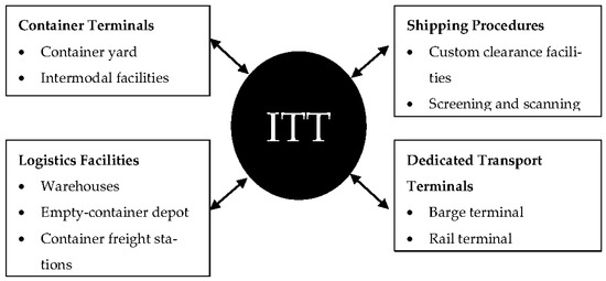
Figure 1.
Role of ITT at seaports (adapted from [2]).
A port provides roads, rails, and barge services to transport containers between terminals and logistics facilities. However, Islam [3] noted that the truck remains the dominant container transportation mode in many ports. For example, at Rotterdam Port, truck transport has a 60% share of the current modal split, the remaining percentage being divided between barge and rail transportation. A similar situation prevails at Hong Kong International Terminal (HIT); according to Murty et al. [4], HIT has more than 200 internal trucks. As many as 10,000 trucks pass through its terminal gate daily. Under these conditions, managing both internal and external trucks is necessary for HIT to maintain its productivity. Increasing the number of internal trucks would be counterproductive for HIT since traffic congestion would increase given its limited space. HIT follows two feasible approaches to solve this problem: reducing the number of vehicles operating in the port and optimizing truck routing. Since ITT is inevitable in most large ports, freight transportation costs have become a crucial economic indicator of supply chain efficiency. Izadi et al. [5] conducted a comprehensive literature review related to freight transportation cost, classified into operational cost, time value, and external cost. Among them, operational cost draws more attention from freight transport operators because it is frequently changing and related to the variable cost, depending on the vehicle’s actual use. This is in contrast to fixed costs such as vehicle insurance, operator license fees, and driver’s wages, which are not affected by the extent of a vehicle’s use. Thus, minimization of operational cost provides more opportunities to reduce the total freight transport cost and maximize profit. Heilig and Voß’s [2] study shows that vehicle routing and scheduling optimization offers many opportunities to reduce operational cost and environmental impact. Many researchers have examined the relation of vehicle routing to scheduling problems. However, most of those studies used a mathematical model and metaheuristics approaches, both of which encounter difficulty in dealing with large-scale problems within a short time.
Furthermore, in a seaport, some logistics facilities have their operational time. In terms of vehicle routing problems, truck waiting time is incurred in cases where a truck arrives at a logistics facility before its opening time. Only a few studies on vehicle routing problems have considered truck waiting time. Moreover, to the best of our knowledge, approaches combining reinforcement learning (RL) with multiagent-based approaches remain limited. In this context, the present study makes the following contributions:
- We propose a cooperative multiagent RL approach to produce feasible truck routes that minimize empty-truck trip cost (ETTC) and truck waiting cost (TWC).
- Under the same ITT-environment characteristics, the learning models produced in this study can provide feasible truck routes in real time within acceptable computational time.
- We conducted computational experiments using artificially generated data and compared the proposed method with two metaheuristic methods, namely simulated annealing (SA) and tabu search (TS), to evaluate the proposed method’s performance.
The rest of this paper is structured as follows: Section 2 is a literature review of the interterminal routing problem, RL for vehicle routing optimization, and multiagent RL. Section 3 presents the concepts of ETTC and TWC in the interterminal truck routing problem (ITTRP). Section 4 discusses the proposed method, which employs cooperative multiagent RL (MARL) to provide feasible truck routes that minimize the ETTC and TWC. Section 5 compares the results of our proposed method with those of the other approaches. Finally, Section 6 draws conclusions and looks ahead to future research.
2. Literature Review
2.1. Interterminal Truck Routing Problem (ITTRP)
Container ports need to handle thousands of containers a day. Those containers might need to be moved from one location to another within a port. In most multiterminal container ports, therefore, ITT is essential to their transportation network. ITT can improve the connectivity between terminals and a port’s logistics facilities and contribute to overall port performance. Since ITT forms a complex network, it needs to be handled efficiently; otherwise, it can be a significant source of transport-related costs. According to Duinkerken et al. [6] and Tierney et al. [7], an efficient ITT system’s main objective is to reduce, minimize, or eliminate transport delay. Another objective of an efficient ITT system is to minimize both transport costs and empty-truck trips [2]. Therefore, designing efficient ITT operations is crucial in order to achieve those objectives and maintain port competitiveness. Heilig and Voß [2] conducted a comprehensive literature review of ITT-related research. One of the ITT-related research opportunities they pointed out is the vehicle routing problem (VRP), which is still not entirely resolved. The VRP offers many opportunities to reduce ITT costs from both economic and environmental perspectives. The approach combining transport scheduling with route optimization provides crucial decision support for terminal operators and third-party operators to increase vehicle utilization and decrease empty-truck trips in ITT networks. Adopting advanced technology is compulsory to cope with dynamic situations and enable real-time tracking and communication with vehicles. In other words, vehicle routing design should be automated such that vehicles can be dynamically dispatched to serve new ITT requests.
The truck routing problem has been studied at the operational level by considering fuel costs, delay costs, emission costs, and ETTC. For example, Jin and Kim [8] studied truck routing at Busan New Port (BNP) with time windows. In their study, the trucking companies collaborate, sharing delivery orders to minimize the number and duration of empty trips. Their proposed mathematical model attempts to maximize trucking company profit by considering truck usage costs and delay penalties. Heilig et al. [9] proposed two greedy heuristics and two hybrid simulated annealing algorithms to generate feasible and improved truck routes within a short computational time. They also developed a mobile cloud platform to facilitate real-time communication for truck drivers and provide context-aware ITT planning for reduced costs and emissions. Heilig et al. [10] proposed a simulated annealing approach to solve a multiobjective ITT truck routing problem by considering truck emissions. Their multiobjective model was designed to minimize the fixed vehicle hiring cost, the vehicle traveling cost, lateness delivery penalty, and emission cost.
2.2. Reinforcement Learning (RL) for Vehicle Routing Optimization
The VRP, with its variants, has been studied for decades. Different approaches such as mathematical models and metaheuristics have been used to tackle it. However, to the best of our knowledge, the utilization of an RL-based approach to handle VRP in the context of ITT is still limited. Mukai et al. [11] adopted and modified a native Q-learning algorithm to deal with on-demand bus systems. In an on-demand bus system, buses pick up customers door-to-door when required. Thus, the bus travel routes are not defined in advance, and the travel route must be changed according to customer occurrence frequency. Native Q-learning needs to be modified to handle this time-dependent problem. The authors improved the Q-value update process and determined the next pickup point based on the time passage parameter. Their proposed algorithm based on Q-learning successfully increases the profit of bus drivers. Jeon et al. [12] applied the Q-learning technique to produce automated guided vehicle (AGV) routes with minimum travel time.
At some container terminals, AGVs are involved in container unloading and loading operations. When a ship arrives at a container terminal, the import containers are lifted by quay cranes (QCs) and handed over to an AGV for transport to the transfer point (TP). In loading operations, an export container is carried by an AGV from the TP to the appropriate QC that loads the container into the specific ship. These AGVs’ operations must be performed efficiently. The proposed Q-learning can derive AGV routes that are 17.3% better than those derived by the shortest-travel-distance technique. Nowadays, a modern transportation service provider requires an efficient technique to design vehicle routing online. Vehicle route generation becomes more computationally complex. Using a mathematical programming approach to manage an extensive transportation network is no longer feasible since it incurs high computational costs. Yu et al. [13] proposed a new deep RL-based neural combinatorial optimization strategy to generate vehicle routing plans with minimal computational time. They devised a deep RL algorithm to determine the neural network model parameters without prior knowledge of the training data’s optimal solutions. They used a real transportation network and dynamic traffic conditions in Cologne, Germany, to evaluate the proposed strategy’s performance. Their proposed strategy can significantly outperform conventional strategies under both static and dynamic conditions. Zhao et al. [14] proposed a novel deep reinforcement learning (DRL) model composed of three components: an actor, an adaptive critic, and a routing simulator. The actor is designed to generate routing strategies based on the attention mechanism. The adaptive critic is devised to accelerate the convergence rate and improve its solution quality during the training process. The final component, the routing simulator, is developed to provide graph information and reward to the actor and adaptive critic. The same authors (Zhao et al. [14]) also combined the proposed DRL model with various local search methods such as Google OR-tools and large neighborhood search (LNS) to yield an excellent solution.
Kalakanti et al. [15] developed RL for the VRP with a two-phase solver to overcome RL’s dimensionality problem. Based on their experiments, the algorithm faces an exploration–exploitation tradeoff when using Q-learning only to solve a VRP. The single-phase solver could not explore enough of the sizeable state-action space to find efficient routes. So, the two-phase solver was designed to mitigate this problem. In the first phase, using geometric clustering, all customer nodes are clustered based on their capacity; in the second phase, Q-learning is used to find the optimal route. The proposed method was compared with the two known heuristics, Clarke–Wright savings and sweep heuristic, to evaluate the proposed method’s performance. The result showed that the proposed method, as compared with the baseline algorithm, can produce an efficient route.
Adi et al. [16] proposed single-agent DRL to solve the VRP in the context of ITT. The authors utilized DRL to provide a feasible truck route with a minimum total cost related to the use of trucks in transporting containers among container terminals. Their experiment used artificially generated data by considering critical information on the container terminal, specifically Busan New Port (BNP). The result shows that their proposed method offers considerable performance in terms of total cost and ETTC compared with the standard algorithms used for solving VRP (i.e., simulated annealing (SA) and tabu search (TS)). However, the proposed method would still require significant modification when used in another case with different container terminal characteristics or to solve a multiobjective problem more likely to arise in an actual container terminal.
2.3. Multiagent Reinforcement Learning (RL)
The increasing complexity of many tasks in various domain problems makes multiagent systems (MASs) attractive to researchers in various disciplines. A MAS consists of autonomous entities known as agents sharing an environment wherein, they receive rewards and take actions. By using a MAS, complex problems are solved by subdividing them into smaller tasks. Most of the complex problems are challenging or even very difficult to solve with a preprogrammed agent. Therefore, an agent should be designed to discover a solution on its own through learning. RL has attracted significant attention to deal with this situation precisely because it can learn by interacting with its environment.
Furthermore, the multiagent RL (MARL) application has recently become prominent in solving complex problems in broad disciplines such as robotics, computer networks, transportation, energy, and economics. Prasad and Dusparic [17] introduced a MARL-based solution for energy sharing between houses in a nearly zero-energy community (nZEC) comprising several zero-energy buildings (ZEBs). This nZEC has an annual total energy use smaller than or equal to the renewable generation within each building. In their study, each building is considered a deep RL agent that learns proper actions to share energy with other buildings. The experimental result showed that the proposed model outperformed the random action selection strategy in the net-zero-energy balance. Calvo and Dusparic [18] proposed the use of an independent deep Q-network (IDQN) to address the heterogeneity problem in a multiagent environment of urban traffic light control. They used dueling double deep Q-networks (DDDQNs) with prioritized experience replay to train each agent for its conditions and consideration of other agents as parts of the environment. A fingerprinting technique enriched the proposed approach for disambiguation of training samples’ age and stabilization of replay memory. The experimental result showed that IDQN is a suitable approach to the optimization of heterogeneous urban traffic control.
The task allocation problem in a distributed environment is one of the most difficult challenges in a MAS. Noureddine et al. [19] proposed a distributed task allocation using cooperative deep RL wherein agents can communicate effectively to allocate resources and tasks. They used the CommNet model [20] to facilitate communication among the agents in requesting help from their cooperative neighbors in a loosely coupled distributed environment. Although their experiment was conducted in a small state-action space, their proposed method was shown to be possible to use in a task allocation problem. For example, the large-scale online ride-sharing platform has a crucial role in alleviating traffic congestion and promoting transportation efficiency in transportation problems. Lin et al. [21] addressed a large-scale fleet management problem using MADRL through two algorithms: contextual deep Q-learning and contextual multiagent actor-critic (AC). These algorithms reallocated transportation resources to balance demand and supply. A parameter-shared policy network in the contextual multiagent AC was used to coordinate the agents, which represented available vehicles. The proposed method showed significant improvement over the state-of-the-art approaches in the authors’ empirical studies.
3. Empty-Truck Trips and Truck Waiting Cost in ITTRP
The ITTRP treated in this study is similar to the homogeneous vehicle pickup and delivery problem with time windows considering several real locations in the Port of Hamburg (Germany) presented by Heilig et al. [22]. Our proposed ITTRP has slightly different characteristics: it does not consider external trucks, and it covers only five real locations containing one container terminal and four logistics facilities at Busan New Port (BNP, Busan, South Korea). As defined, the ITTRP moves containers between facilities within a port using a transport mode. Heilig et al. [22] defined ITTRP as follows:
| L | Set of locations |
| T | Set of trucks |
| C | Set of customers |
| Set of requesting transport orders (TOs) of customers. , where k is The index of the customer | |
| O | Set of all requesting orders, where |
| Origin (source) location of a TO, where | |
| Destination location of a TO, where | |
| Subsets of the origin (source) location | |
| Subsets of the destination location | |
| Service time at origin (source) location of a TO | |
| Service time at destination location of a TO | |
| TO due date | |
| Penalty cost for late TO, based on the due date | |
| An initial position of a truck | |
| Maximum number of working hours | |
| A prefixed cost for using a truck | |
| Variable costs per hour |
The empty-truck trip cost (ETTC), , is incurred when the truck’s current position is different from the TO’s origin to be served; therefore, to pick up a container, the truck must travel to the TO’s origin from its current position without bringing any container. Equation (1) calculates the ETTC as
where spd is the standard truck speed set to 40 km/h and ec is the cost per hour that is applied when the truck travels from one location to another without any container. Each location in the port has an opening and closing time restricting the arrival of trucks. Truck waiting time is incurred when the truck arrives at the TO’s origin earlier than its opening time. This truck waiting time will be converted to a truck waiting cost (TWC), , that is determined by multiplying the former by the waiting cost per hour, wch, as shown in Equation (2):
where is the opening time at the origin location of the TO and is the arrival time of a truck at the TO’s origin. The objective of this problem is to minimize the costs related to the use of trucks, which also include the ETTC and the TWC. This is shown in the objective function
where is equal to 1 if truck t is hired and 0 otherwise; is equal to 1 if the TO o is performed after its due date and 0 otherwise. The service time required by a truck t for performing all of its assigned TOs is denoted as . is equal to 1 if the execution of TO o produces an ETTC and 0 otherwise. is equal to 1 if the execution of TO o produces waiting time and 0 otherwise. A solution to the ITTRP must satisfy the following feasibility restrictions:
- All TOs must be served.
- A TO must be performed by a single truck.
- Each TO must be performed by considering its due date, including the service time at origin (source) and destination locations. The penalty cost is applied to every TO that is served after its due date.
- The initial position of all trucks is at terminal 1, and the next starting point of each truck is the destination location of the latest order served by the truck. The time and cost required for moving trucks from the initial location to the order origin (for first-time order assignments) are not considered objective.
- Pickup and delivery operations are considered as pairing constraints in the TO.
- The pickup vertices are visited before the corresponding delivery vertices (precedence constraints).
- Each location has a given availability time window; hence, the trucks can arrive at the origin and destination based on their given time windows. When trucks arrive in advance, they must wait until the opening time for the pickup or delivery.
The following assumptions are applied:
- The truck speed and distance between the terminals, which are used to calculate the travel time as well as service time and time windows, are known in advance.
- The fee for carrying out TOs, fixed costs, and variable costs are known in advance.
Based on [23,24], this problem can be seen as a multidepot pickup and delivery problem with time windows (MDPDPTW) at the origins and destinations. Let be the set of all feasible routes performed by truck from its origin location . A binary variable, , is associated with each route and indicates that a route is selected. For each order, let be a binary coefficient with value 1 if and only if order is performed on route r. Moreover, is the overall cost of route r, considering the cost according to (3). In order to include the possibility of more than one truck being available at a given starting position , the parameter is included as an upper bound on the number of trucks. Given the above definitions, the integer linear model can be formulated as follows:
subject to
Objective (4) aims to minimize the overall cost of the selected routes. Constraints (5) are standard set partitioning constraints ensuring that each TO is performed. The set of constraints (6) establishes the limitation on the maximum number of available trucks at each starting location. Constraints (7) are binary restrictions on the decision variable.
4. Proposed Method
4.1. Reinforcement Learning (RL)
The recent advance in computer technology provides great computing power for developing the artificial intelligence (AI) field. Machine learning (ML) is an AI field that has recently attracted significant attention from many academics and researchers. There are three approaches in ML, supervised learning (SL), unsupervised learning (UL), and reinforcement learning (RL). Each approach has its characteristics and objective in solving a problem. SL usually use to predict an output variable from high-dimensional observations. A famous example of SL is handwritten-digit recognition. The trained SL model learns from labeled data and is expected to classify a new handwritten digit image correctly.
In contrast to SL, UL acts unsupervised to discover hidden structures or patterns from unlabeled data. In the real world, the case is not always about prediction or finding the patterns from data. Some problems should be solved by involving sequential decision-making. Unfortunately, SL and UL are not fit for solving this kind of problem. RL emerges to tackle the sequential decision-making problems. RL was inspired by how human beings learn something through an interaction with the environment and improve their decision based on signals considered positive or negative rewards. Figure 2 shows the two essential components in RL, an agent and an environment. An RL agent learns through continuous trial-and-error interaction with an environment. As a response to the RL agent, the environment provides a numerical reward and a new state every time an RL agent executes an action. An RL agent performs this learning cycle within a finite or infinite horizon.
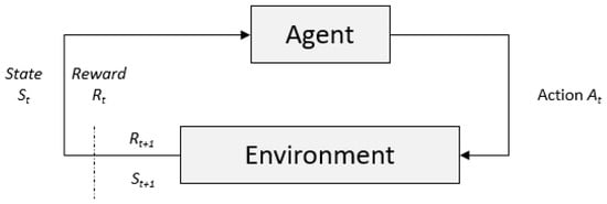
Figure 2.
Agent–environment interaction in RL (adapted from [25]).
The RL problem is formally defined in the form of a Markov decision process (MDP), which is described as a tuple , where:
- is the set of the possible state of the environment that is defined as a finite state.
- is the set of possible actions that can be executed by an agent to interact with the environment.
- denotes the transition probability to move to the state and receiving a reward, r, given as follows: .
- is the expected reward received from the environment after the agent performs action a, at state s.
- is a discount factor determining how far the agent should look into the future.
The ultimate goal of RL is to find the optimal policy π, that maximizes the expected return. The expected return over a finite length of time horizon defined as follows:
where is a discount with the following value range . The expected return in the Q-learning algorithm under a policy π is defined as
where is the discounted future reward when an agent executes action a, in state s. The maximal action value for executing action a, in state s, achievable by any policy, is defined as follows:
By definition, policy π is a function that defines the probability of choosing action a, in state s: S → p (A = a|S). In our case, the best policy is determined by utilizing a deep neural network because the case study is considered as a high-dimensional state-action space. The detailed design of each state, action, and reward is discussed in the following subsection.
4.2. Deep Q-Network
The RL algorithm has been employed for decades to solve various sequential decision-making problems. Using model-free algorithms such as Q-learning that rely on the q-table to store a q-value representing the best action from a particular state has not been strongly recommended to overcome the large-scale problem. The combination of deep learning (DL) and RL, called deep reinforcement learning (DRL), offers an advantage to cope with the curse of dimensionality. DL has an important property that can automatically find compact low-dimensional representations of high-dimensionality data such as images, text, and audio [26]. Deep Q-network (DQN), a novel structure that combines RL and a convolutional neural network (CNN) proposed by Mnih et al. [27], was successfully proved in making an autonomous agent play a series of 49 Atari games. The authors applied CNN in a DQN to interpret the graphical representation of the input state, s, from the environment. For the same reason, in this study, we utilized a DQN to solve our problem, mainly since the state-action space was considerably large in our case. The difference from the work of Mnih et al. [27] is that we do not incorporate CNN architecture. Our custom state design is fed directly as an input for the deep Q-network shown in Figure 3.
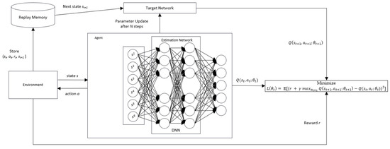
Figure 3.
Deep Q-network structure [16].
Figure 3 illustrates the DQN structure, a model-free RL that uses a DNN as a policy-approximation function. is represented as an approximator with parameter and needs to approach the optimal action value, that is,
where parameters are learned iteratively by minimizing the loss function
where is the target value and and represent the state and action at time step t + 1, respectively. The target value must be replaced with weight , which is updated at every N step from the estimation network to address the instability issue in the DQN. Therefore, the loss function is updated as follows:
Moreover, an experience replays memory store generated samples . These samples are then retrieved randomly from the experience replay and fed into the training process.
4.3. Cooperative Multiagent Deep Reinforcement Learning (DRL)
In our case study, the use of single-agent RL led to a sizeable state-action space (33,177,600 combinations of all possible states and actions), thus rendering the agent unable to learn efficiently. Moreover, relying on single-agent RL to achieve two objectives will also decrease the agent’s learning effectiveness. We propose a cooperative multiagent deep RL (CMADRL) that contains two agents focusing on a specific objective to cope with this situation. Figure 4 shows the cooperative multiagent (DRL) architecture used in our case study. Our proposed method’s cooperative term determines that the first and second agents must cooperate to produce a truck route with minimum ETTC and TWC.
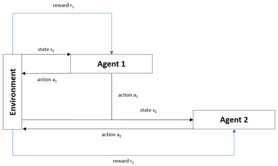
Figure 4.
Cooperative multiagent deep reinforcement learning (DRL) architecture.
In other words, the decision process is executed in the following sequence: The first agent will evaluate the given state to decide the best action to be taken, and the selected action will then be a part of the second agent’s state. After that, the second agent will decide the best action that should be taken to achieve the second objective. Since the state-action space is considerably large, each agent employs DRL as a policy approximation function.
4.3.1. Agent 1 Design
In the ITTRP, an agent (a truck) observes a state received from its environment to take action. In the state, three parameters are critical in decision-making related to minimizing ETTC: time, truck position, and the TO characteristics (TOCs). A truck must consider the available TO at time t and the TOCs based on the distance ratio. The first agent has an objective to select the TO that minimizes the ETTC. The agent should choose the TO with the minimal distance ratio (DR) to achieve this objective. Figure 5 illustrates how the DR is calculated and its relationship with the ETTC category. Assume that we have five locations, including three container terminals and two logistics facilities, described as T1, T2, T3, F1, and F2: the distance between the terminals is 1 unit. Therefore, in this case, the longest distance is traveling from T1 to F2, which is four units. At time t, the current truck position (CTP) is at T1. Furthermore, at the same time, there are three available TOs.
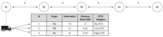
Figure 5.
Example of distance ratio and ETTC category based on the distance ratio.
Using Equation (14), we can obtain 0, 0.25, and 0.75 as the DRs for TO 1, TO 2, and TO 3, respectively. The DR is vital to determining the category of ETTC. The ETTC category defines the level of the TO’s ETTC. The higher the DR, the higher the ETTC. Furthermore, the agent should learn to choose the lowest DR as often as possible so that the total ETTC serving the TO is minimal. In the implementation, based on the DR, we define three transport order characteristics (TOCs): the TO with DR of zero (TOC1), the TO with DR of more than 0 and less than 0.50 (TOC2), and the TO with DR more than 0.50 (TOC3).
State Representation
From the previous explanation, we can conclude that the state for agent 1 should include five essential elements, SM = {, , , , }, where:
- represents the current time in minutes. The value has a range of 0–1440 that represents a 24 h range in minutes.
- represents the position of the truck. In our case, we only cover three terminals and two logistics facilities. The value of this element has a range of 1 to 5.
- indicates the presence of a TO with DR equal to 0.
- indicates the presence of a TO with DR > 0 and <= 0.50.
- indicates the presence of a TO with DR of more than 0.50.
Actions
Agent 1 can choose three possible actions at each time step t; therefore, a set of actions of agent 1, , consists of three elements, , where:
- : choose TO with TOC1 characteristics.
- : choose TO with TOC2 characteristics.
- : choose TO with TOC3 characteristics.
Rewards
A proper reward function design is vital in RL to induce an agent to maximize the cumulative reward. An environment provides feedback in the form of a reward to an agent after executing an action. For agent 1, the ultimate goal is to pick the TO with the minimum ETTC. In this study, we propose four reward cases at each time step:
- R(t) = 0.01, if an agent takes no action when there is no TO.
- R(t) = −0.1, if an agent performs an improper action such as choosing , or when the TO with the corresponding characteristics is not available.
- R(t) = 100, if the selected action results in ETTC = 0.
- R(t) = 50, if the selected action results in ETTCi <= AETTC, where ETTCi is the current ETTC and AETTC is the average of the empty-truck trip costs of all complete TOs.
The first reward case is when the agent chooses to remain idle when there are no available TOs at the current time. The reward value is deliberately set to a small amount, such as 0.01, to prevent the agent from considering it as the best action when performed repeatedly. Unwanted behavior will arise when its cumulative reward beats the reward of taking the expected action. The second reward case was designed to make an agent avoid undesirable behavior. A negative reward will be given when the agent takes improper action, categorized in the second reward case above. For example, the agent will obtain minus 0.1 when it takes no action while, at the current time, there are available TOs. The third and fourth reward cases define the immediate reward. Both of them are designed to give a reward for the expected action selection. The third case will be given to the agent when the selected action results in zero ETTC, while the fourth case will be given when the chosen action results in an ETTC that is less than or equal to the average of all served TOs.
4.3.2. Agent 2 Design
After the first agent makes a decision, agent 2 decides to take action based on another perspective of judgment, the time perspective, by which it attempts to choose the TO that minimizes truck waiting time. The first agent’s decision affects the availability of the TO that can be chosen by agent 2. Suppose that the first agent chooses to serve TO 1 with origin locations the same as the current truck locations (see Figure 5), which is T1. Therefore, the available TOs to be selected by agent 2 are the TO with T1 as its original location, as shown in Figure 6. Knowing the TOs’ waiting time ratio (WTR) is vital for the second agent to achieve the objective. Truck waiting time occurs when a truck arrives in advance at a TO origin. Here, agent 2 observes two WTRs: origin waiting time ratio (OWTR) and destination waiting time ratio (DWTR). These ratios are essential in order to identify whether the TO will result in TWC or not. The following equations obtain OWTR and DWTR:
where is the opening time at the TO origin location, is the opening time at the TO destination location, is the arrival time of a truck at the TO’s origin, is the arrival time of a truck at the TO’s destination, and is the waiting time threshold indicative of a truck’s maximum acceptable waiting time at the TO origin/destination, 60 min being the default value.
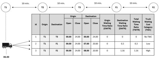
Figure 6.
Waiting time ratio (WTR) and truck waiting cost (TWC).
Figure 6 is a simplified example showing five locations containing three terminals (T1, T2, T3) and two logistics facilities (F1, F2), the travel time between locations being 10 min. The CTP is at T1, and the current time is 06.00. At that time, there were three options for the available TOs. The OWTR for all TOs is 0 because the TO origin, T1, operates for 24 h. Under the assumption of 10 min for the container loading process, we can obtain DWTR as 0, 0.3, and 1.16 for TOs 1, 2, and 3, respectively. The total waiting time ratio (TWTR) is a summation of OWTR and DWTR. The TWTR is used to determine the TWC categories. If the TWTR is equal to 0, it is categorized as no TWC (NTWC); if it is more than 0 and less than 1, it is categorized as low TWC (LTWC); and if it is more than 1, it is categorized as high TWC (HTWC). Choosing the TO with no TWC or LTWC is agent 2’s expected action to achieve the objective.
State Representation
The state representation of agent 2 is similar to that of agent 1. The differences are in the TOCs, and agent 2’s state includes an action taken by agent 1. In agent 1’s state, there are three TOCs from a distance perspective, called the DR ratio. However, in agent 2’s state, we replace those three TOCs with the TWC perspective, which contains six elements, SW = {, , , , , }, where:
- means that an action was taken by agent 1.
- represents the current time in minutes. The value has a range of 0–1440 that represents a 24 h duration in minutes.
- represents the current position of the truck. In our case, we covered only one terminal and four logistics facilities. The value of this element has a range of 1 to 5.
- indicates the presence of a TO with NTWC characteristics.
- indicates the presence of a TO with LTWC characteristics.
- indicates the presence of a TO with HTWC characteristics.
Actions
Agent 2 can choose three possible actions at each time step t; therefore, a set of actions of agent 2, , consists of three elements, , where:
- : choose a TO with NTWC characteristics.
- : choose a TO with LTWC characteristics.
- : choose a TO with HTWC characteristics.
Rewards
Agent 2’s objective is to pick up the TO that minimizes the TWC; therefore, agent 2’s reward design should support the agent’s learning and achieving the objective. There are three reward cases for agent 2, as follows:
- R(t) = −0.1, if an agent chooses action , , or when the TO with the corresponding characteristics is not available.
- R(t) = 100, if the selected action results in TWC = 0.
- R(t) = 50, if the selected action results in TWCi <= ATWC, where TWCi is the current TWC and ATWC is the average of all complete TOs’ TWCs.
The TO options for agent 2 are limited because the options already filter out based on agent 1’s selected TOs. The remaining options are to choose the TO with LTWC or HTWC characteristics. The first case reward attempts to punish the agent with a negative reward for choosing action when the TO with LTWC characteristics is not available and likewise punishes the agent for choosing action or when the TO with the corresponding characteristics is not available. The last two reward cases encourage the agent when choosing an action that meets the agent’s objective. The agent will receive 100 as a reward if the selected action produces zero for TWC and 50 if the TWC is less than or equal to the average of the TWCs of all complete TOs.
5. Experimental Results
Simulation experiments were conducted to evaluate the performance of the proposed method. All of the algorithms were implemented using Python version 3.7 and run on a PC equipped with an Intel Xeon CPU E3-1230 v5 of 3.40 GHz and 32 GB memory. In the training phase, we trained our DQN using 500 files, where each file contains 285 TO data, as illustrated in Table 1, and runs for 1000 episodes. The number of files used in the training process represents the TO data’s different variation characteristics that might occur in the actual container terminal. The variation of training data is required to allow an agent to learn by experience in finding the optimal policy from different circumstances. It takes 350 h (approximately 14.5 days) to complete the training process of 500 files with 1000 episodes per file. At the end of the training process, two RL models were produced: a model that can minimize the ETTC and another that can minimize the TWC. These two models were later used in the testing phase, which follows the scenario described in Figure 7.

Table 1.
Example of TO data.
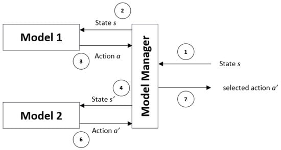
Figure 7.
Model manager in the testing phase.
As illustrated in Figure 7, the model manager will direct the state s to the first model, which is responsible for making a decision that minimizes the ETTC and feeds the result to the model manager. Then, the model manager will produce a proper state for the second model, which is responsible for making a decision that minimizes TWC. The decision made by the second model considered the final decision (selected action).
5.1. Data
The data used in this experiment were artificially generated by considering some critical properties of the actual container terminal (BNP). The TO data contain four essential elements in the ITTRP: the TO origin, TO destination, start time window, and due date, as shown in Table 1. The value ranges of the respective elements are as follows:
- TO origin (o): {T1, T2, T3, F1, F2}.
- TO destination (d): {T1, T2, T3, F1, F2}, where d ≠ o.
- Start time window (in minutes): {0, …, 1320}.
- Due date (in minutes): {120, …, 1440}.
In BNP, the longest travel time is 58 min to travel from one location to another. The determination of the start time window and due date consider this travel time. The start time window can be started from time 0, but it is not logical if the due date starts from time 0. The same rule was also applied to determine the maximum value of the start time window and the due date. The 120 gaps for the maximum time window value and the minimum due date value are determined based on 2 times the longest travel time.
We used five places, namely three container terminals denoted by T1, T2, and T3 and two logistics facilities denoted by F1 and F2. Each TO describes a container transport task performed by a truck from origin to destination between the start time window and the due date. The container terminal operates for 24 h, and so the operational time is from 00.00 to 24.00. The logistics facilities have different operational times from those of the terminals, as shown in Table 2.
Table 2.
Operational times of terminals and logistics facilities.
The generated data included actual information from a seaport, which in our case was Busan New Port (BNP). The five facilities’ locations used in our case are the actual locations within BNP: T1, T2, T3, F1, and F2 corresponded exactly to PNIT, PNC, HJNC, HPNT, and BNCT, respectively, in BNP (see Figure 8). Additionally, as shown in Table 3, we used the same container movement rates between BNP terminals as Park and Lee [28] published.
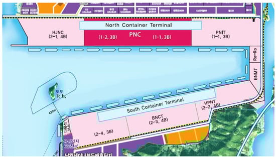
Figure 8.
Busan New Port (BNP) container layout [28].
Table 3.
Container movement rates between terminals in BNP [28].
To provide a near-real simulation environment for our proposed RL, we used two crucial pieces of information: container processing time and the standard cost and fee. The container processing time information includes terminal-to-terminal travel time (T2T), the time required for traffic lights (TRTL), gate passing time (GPT), and waiting time for loading/unloading (WTUL), as shown in Table 4 as taken from the work of Park and Lee [28].
Table 4.
Estimated container processing times per move [28].
Standard costs and fees are required to calculate the truck-related costs for every transport task performed by a truck. We used the standard published by Jin and Kim [8], which includes the truck transport cost, idle cost, delay cost, and revenue per container, as shown in Table 5. The term of one time period in Table 5, refers to a 15 min time unit. For example, a truck transportation cost of 4 USD/time-period means that the transportation cost is USD 4 for every 15 min. Since we did not have any information on the TWC, we used the idle cost, which is USD 0.01 for one time period, to calculate the TWC in our experiment.
Table 5.
Standard costs and fees [8].
Dataset variation is crucial to the performance evaluation process of the proposed method. As shown in Table 6, we used three dataset categories determined based on our experiment’s number of TOs (i.e., 3).
Table 6.
Datasets for experiment [16].
5.2. Algorithm Configuration
5.2.1. DQN Configuration
In this experiment, we employed KERAS library version 2.3 to develop a DL for use in our proposed DQN. The DL model for each agent, particularly the number of neurons for the input and output layers, was determined based on each agent state and action design, as explained in Section 4.3.1 and Section 4.3.2. The first agent had five neurons and three neurons for its input and output layers, while the second agent had six and three. However, both agents used the same configuration for the hidden layer: two hidden layers with nine neurons for each layer. The determination of the number of hidden neurons was based on the following rule of thumb [29]:
- The number of hidden neurons should be between the input layer’s size and the output layer’s size.
- The number of hidden neurons should be two-thirds of the input layer’s size plus the size of the output layer.
- The number of hidden neurons should be less than twice the size of the input layer.
All of the hidden layers used a rectified linear activation function, whereas the output layer used a linear activation function. The DQN hyperparameters were set with specific values in the training process, as shown in Table 7. The DQN was trained using a 500-dataset variation of TOs. Each variation contained 35 to 285 transport data and ran for 1000 episodes. In other words, roughly, the DQN trained for 500,000 episodes. This dataset variation was intended to make the DQN learn from many experiences.
Table 7.
DQN hyperparameters.
5.2.2. Simulated Annealing (SA) Configuration
Simulated annealing (SA) is the standard algorithm usually utilized to solve the VRP. The SA algorithm is a local search heuristic that uses a probability function to accept a worse solution to escape from local optima. The algorithm was proposed by Kirkpatrick et al. [30], who had been inspired by the annealing process of metal, which starts at a high temperature and slowly decreases the temperature until it reaches a defined lowest state. In this experiment, we used standard SA with a random neighborhood structure, including swap and insertion. The initial temperature (Tinitial) of the SA was set to 100 degrees, the cooling rate (α) was calculated using the following equation , and the stopping criterion was set as a temperature (Tfinal) of 0.0001 degrees. The Boltzmann probability was used to accept the new solution. If this probability was higher than a random value between 0 and 1, the new solution was accepted. The determination of the initial and final temperatures was based on [31], which states that a broader gap between the initial and final temperatures might give SA adequate time for leaving local optima. Furthermore, the number of iterations for the SA algorithm was set based on [32], which suggested that for a candidate size of 285 (as in our case study), 100,000 iterations are sufficient.
5.2.3. Tabu Search (TS) Configuration
The second standard algorithm used to evaluate the proposed method’s performance was tabu search (TS). TS is a metaheuristic algorithm designed to guide subordinate heuristic search process to escape from local optima. The original form of the TS algorithm was proposed by Glover [33]. Two features, namely a memory mechanism and tabu criteria, distinguish TS from other metaheuristics. These features give TS the capability to avoid the circuitous condition. TS used the aspiration criterion to ensure a diversified search and obtainment of the global optimum. In our experiment, we set the length of the tabu list to seven. We use the same value for the number of iterations we set for SA, 100,000, since the candidate size was the same. The neighborhood search method was used for both SA and TS; we used two transformation rules for the generation of neighbors, as proposed by Tan [34]. The first rule is exchanging routes within a vehicle, and the second rule is exchanging routes between two vehicles. The new solution obtained from the generation of neighbors was evaluated to meet the primary objective function: minimization of ETTC and TWC.
5.3. Results
In the training phase, we evaluated the performance of the RL agent by observing the reward obtained and the costs (ETTC and TWC) produced in every episode. The performance result was taken from the training process using the DC3-285 dataset. The performances of agents 1 and 2 shows in Figure 9 and Figure 10, respectively, in terms of reward obtained in each episode for 1000 episodes. The x-axis in both figures presents the number of episodes, and the y-axis shows the cumulative reward per episode. Both agents could quickly recognize the best action leading to high reward within less than 150 episodes. However, their performances after episode 150 showed no significant improvement until the end of the episodes. This reward performance was consistent with the cost performance, as shown in Figure 11 and Figure 12. The cost decreased when the agent successfully increased the reward and vice versa.
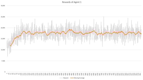
Figure 9.
Cumulative reward per episode of agent 1.
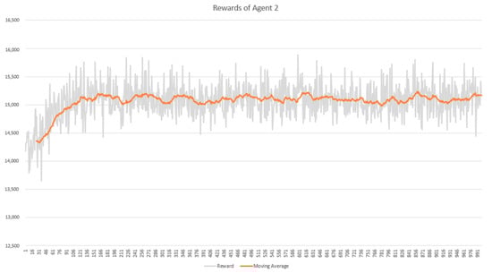
Figure 10.
Cumulative reward per episode of agent 2.
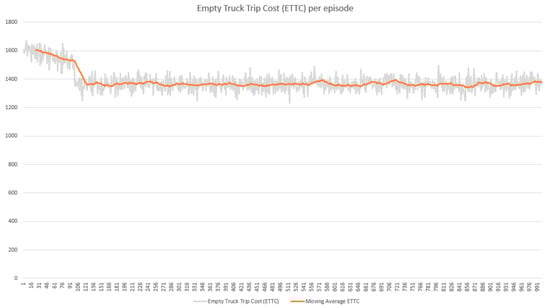
Figure 11.
Empty-truck trip cost (ETTC) per episode.
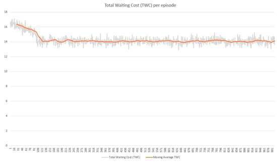
Figure 12.
Truck waiting cost (TWC) per episode.
In the testing phase, we ran the DQN and the two baseline algorithms 30 times for each dataset shown in Table 6. At the end of every test, we obtained the minimum and average values of the three performance parameters: TWC, ETTC, and computational time. The list of performance parameter abbreviations in Table 8 can be considered to apply to Table 9 and Table 10.
Table 8.
Performance parameter abbreviations.
Table 9.
Performance comparison between DQN and SA.
Table 10.
Performance comparison between DQN and TS.
Table 9 shows that, overall, the proposed DQN achieved a better result than SA for all datasets. The proposed DQN can determine truck routing with minimum TWC and ETTC in less computational time than SA. A similar result was seen when comparing DQN with TS, as shown in Table 10.
The proposed DQN dominated almost all of the performance parameters. However, for the last two datasets, DC2-173 and DC3-285, it could do only slightly better than TS in terms of TWC and ETTC (Table 11). This might have been due to the inadequate dataset variety for DC2-173 and DC3-285, in which case it would seem that the proposed DQN cannot obtain significant improvement over TS in the testing phase.
Table 11.
Performance gaps between DQN and SA and between DQN and TS.
6. Conclusions
In optimizing the interterminal truck routing problem (ITTRP), achieving more than one objective is possible. A single-agent RL cannot solve the multiobjective problem efficiently since that problem will produce a high-dimensional state-action space that requires much computational time. This study attempted to solve the multiobjective problem of minimizing empty-truck trip cost (ETTC) and truck waiting cost (TWC). Cooperative multiagent deep reinforcement learning (CMADRL), consisting of two agents focused on a specific objective, solved the multiobjective problem. The first agent focused on minimizing the ETTC, while the second agent focused on minimizing the TWC by considering the first agent’s decision to take further action. The experimental result showed that the proposed CMADRL could produce better results than the baseline algorithms. The proposed method could reduce the TWC and ETTC by up to 22.67 and 25.45%, respectively, compared with simulated annealing (SA) and tabu search (TS). Although the proposed method achieved good results, there are still several challenges for future studies. First, as the proposed method was not designed for a general ITTRP in many container terminals, it will require significant modifications to solve similar problems. The ITT problem considered in this study involved only homogeneous vehicles, which cannot realistically represent the current modern container terminal, which usually utilizes a heterogeneous fleet. Furthermore, the proposed RL still requires significant training time and is dependent on a vast training dataset. These problems should receive serious attention to enhance the proposed method’s practicality for solving real-world problems.
Author Contributions
Conceptualization, writing—original draft preparation, T.N.A.; review and editing, Y.A.I.; supervision and review, H.B. All authors have read and agreed to the published version of the manuscript.
Funding
This research was supported by the MSIT (Ministry of Science and ICT), Korea, under the Grand Information Technology Research Center support program (IITP-2021-2016-0-00318) supervised by the IITP (Institute for Information & communications Technology Planning & Evaluation) and in part of the research project of ‘Development of IoT Infrastructure Technology for Smart Port’ funded by the Ministry of Oceans and Fisheries, Korea.
Institutional Review Board Statement
Not applicable.
Informed Consent Statement
Not applicable.
Data Availability Statement
Not applicable.
Conflicts of Interest
The authors declare no conflict of interest.
References
- UNCTAD. Review of Maritime Transport 2018; Review of Maritime Transport; UNCTAD: Geneva, Switzerland, 2018; ISBN 9789210472418. [Google Scholar]
- Heilig, L.; Voß, S. Inter-terminal transportation: An annotated bibliography and research agenda. Flex. Serv. Manuf. J. 2017, 29, 35–63. [Google Scholar] [CrossRef]
- Islam, S. Transport Capacity Improvement in and around Ports: A Perspective on the Empty-Container-Truck Trips Problem. Ph.D. Thesis, The University of Auckland, Auckland, New Zealand, 2014. [Google Scholar]
- Murty, K.G.; Wan, Y.W.; Liu, J.; Tseng, M.M.; Leung, E.; Lai, K.K.; Chiu, H.W.C. Hongkong international terminals gains elastic capacity using a data-intensive decision-support system. Interfaces 2005, 35, 61–75. [Google Scholar] [CrossRef] [Green Version]
- Izadi, A.; Nabipour, M.; Titidezh, O. Cost Models and Cost Factors of Road Freight Transportation: A Literature Review and Model Structure. Fuzzy Inf. Eng. 2020, 1–21. [Google Scholar] [CrossRef]
- Duinkerken, M.B.; Dekker, R.; Kurstjens, S.T.G.L.; Ottjes, J.A.; Dellaert, N.P. Comparing transportation systems for inter-terminal transport at the Maasvlakte container terminals. OR Spectr. 2006, 28, 469–493. [Google Scholar] [CrossRef]
- Tierney, K.; Voß, S.; Stahlbock, R. A mathematical model of inter-terminal transportation. Eur. J. Oper. Res. 2014, 235, 448–460. [Google Scholar] [CrossRef]
- Jin, X.; Kim, K.H. Collaborative inter-terminal transportation of containers. Ind. Eng. Manag. Syst. 2018, 17, 407–416. [Google Scholar] [CrossRef]
- Heilig, L.; Lalla-Ruiz, E.; Voß, S. Port-IO: A mobile cloud platform supporting context-aware inter-terminal truck routing. In Proceedings of the 24th European Conference on Information Systems, ECIS 2016, Istanbul, Turkey, 12–15 June 2016. [Google Scholar]
- Heilig, L.; Lalla-Ruiz, E.; Voß, S. Multi-objective inter-terminal truck routing. Transp. Res. Part E Logist. Transp. Rev. 2017, 106, 178–202. [Google Scholar] [CrossRef]
- Mukai, N.; Watanabe, T.; Feng, J. Route optimization using Q-learning for on-demand bus systems. In International Conference on Knowledge-Based and Intelligent Information and Engineering Systems; Springer: Berlin/Heidelberg, Germany, 2008. [Google Scholar]
- Jeon, S.M.; Kim, K.H.; Kopfer, H. Routing automated guided vehicles in container terminals through the Q-learning technique. Logist. Res. 2011, 3, 19–27. [Google Scholar] [CrossRef]
- Yu, J.J.Q.; Yu, W.; Gu, J. Online Vehicle Routing With Neural Combinatorial Optimization and Deep Reinforcement Learning. IEEE Trans. Intell. Transp. Syst. 2019, 20, 3806–3817. [Google Scholar] [CrossRef]
- Zhao, J.; Mao, M.; Zhao, X.; Zou, J. A Hybrid of Deep Reinforcement Learning and Local Search for the Vehicle Routing Problems. IEEE Trans. Intell. Transp. Syst. 2020, 1–11. [Google Scholar] [CrossRef]
- Kalakanti, A.K.; Verma, S.; Paul, T.; Yoshida, T. RL SolVeR Pro: Reinforcement Learning for Solving Vehicle Routing Problem. In Proceedings of the 2019 1st International Conference on Artificial Intelligence and Data Sciences (AiDAS), Ipoh, Malaysia, 19 September 2019; pp. 94–99. [Google Scholar]
- Adi, T.N.; Iskandar, Y.A.; Bae, H. Interterminal truck routing optimization using deep reinforcement learning. Sensors 2020, 20, 5794. [Google Scholar] [CrossRef]
- Prasad, A.; Dusparic, I. Multi-agent Deep Reinforcement Learning for Zero Energy Communities. In Proceedings of the 2019 IEEE PES Innovative Smart Grid Technologies Europe (ISGT-Europe), Bucharest, Romania, 29 September–2 October 2019; pp. 1–5. [Google Scholar]
- Calvo, J.A.; Dusparic, I. Heterogeneous multi-agent deep reinforcement learning for traffic lights control. CEUR Workshop Proc. 2018, 2259, 2–13. [Google Scholar]
- Ben Noureddine, D.; Gharbi, A.; Ben Ahmed, S. Multi-agent Deep Reinforcement Learning for Task Allocation in Dynamic Environment. In Proceedings of the 12th International Conference on Software Technologies, Madrid, Spain, 24–26 July 2017; pp. 17–26. [Google Scholar]
- Sukhbaatar, S.; Szlam, A.; Fergus, R. Learning multiagent communication with backpropagation. Adv. Neural Inf. Process. Syst. 2016, 2252–2260. [Google Scholar] [CrossRef]
- Lin, K.; Zhao, R.; Xu, Z.; Zhou, J. Efficient Large-Scale Fleet Management via Multi-Agent Deep Reinforcement Learning. In Proceedings of the 24th ACM SIGKDD International Conference on Knowledge Discovery & Data Mining, London, UK, 19–23 August 2018; pp. 1774–1783. [Google Scholar]
- Heilig, L.; Lalla-Ruiz, E.; Voß, S. port-IO: An integrative mobile cloud platform for real-time inter-terminal truck routing optimization. Flex. Serv. Manuf. J. 2017, 29, 504–534. [Google Scholar] [CrossRef]
- Min, H. The multiple vehicle routing problem with simultaneous delivery and pick-up points. Transp. Res. Part A Gen. 1989, 23, 377–386. [Google Scholar] [CrossRef]
- Bettinelli, A.; Ceselli, A.; Righini, G. A branch-and-cut-and-price algorithm for the multi-depot heterogeneous vehicle routing problem with time windows. Transp. Res. Part C Emerg. Technol. 2011, 19, 723–740. [Google Scholar] [CrossRef]
- Sutton, R.S.; Barto, A.G. Reinforcement Learning: An Introduction, 2nd ed.; MIT Press: London, UK, 2018; ISBN 978-0262039246. [Google Scholar]
- Arulkumaran, K.; Deisenroth, M.P.; Brundage, M.; Bharath, A.A. Deep Reinforcement Learning: A Brief Survey. IEEE Signal Process. Mag. 2017, 34, 26–38. [Google Scholar] [CrossRef] [Green Version]
- Mnih, V.; Kavukcuoglu, K.; Silver, D.; Rusu, A.A.; Veness, J.; Bellemare, M.G.; Graves, A.; Riedmiller, M.; Fidjeland, A.K.; Ostrovski, G.; et al. Human-level control through deep reinforcement learning. Nature 2015, 518, 529–533. [Google Scholar] [CrossRef] [PubMed]
- PARK, N.-K.; LEE, J.-H. The Evaluation of Backhaul Transport with ITT Platform: The Case of Busan New Port. J. Fishries Mar. Sci. Educ. 2017, 29, 354–364. [Google Scholar] [CrossRef]
- Tamura, S.; Tateishi, M. Capabilities of a four-layered feedforward neural network: Four layers versus three. IEEE Trans. Neural Netw. 1997, 8, 251–255. [Google Scholar] [CrossRef]
- Kirkpatrick, S.; Gelatt, C.D.; Vecchi, M.P. Optimization by simulated annealing. Science 1983, 220, 671–680. [Google Scholar] [CrossRef] [PubMed]
- Weyland, D. Simulated annealing, its parameter settings and the longest common subsequence problem. In Proceedings of the 10th Annual Conference on Genetic and Evolutionary Computation, Atlanta, GA, USA, 12–16 July 2008; p. 803. [Google Scholar]
- Fu, Q.; Zhou, K.; Qi, H.; Jiang, F. A modified tabu search algorithm to solve vehicle routing problem. J. Comput. 2018, 29, 197–209. [Google Scholar] [CrossRef]
- Glover, F. Future paths for integer programming and links to artificial intelligence. Comput. Oper. Res. 1986, 13, 533–549. [Google Scholar] [CrossRef]
- Kokubugata, H.; Kawashim, H. Application of Simulated Annealing to Routing Problems in City Logistics. In Simulated Annealing; InTech: Vienna, Austria, 2008; ISBN 9789537619077. [Google Scholar]
Publisher’s Note: MDPI stays neutral with regard to jurisdictional claims in published maps and institutional affiliations. |
© 2021 by the authors. Licensee MDPI, Basel, Switzerland. This article is an open access article distributed under the terms and conditions of the Creative Commons Attribution (CC BY) license (https://creativecommons.org/licenses/by/4.0/).