Building Robust Closed-Loop Supply Networks against Malicious Attacks

Abstract

With recent industrial upgrades, it is essential to transform the current forward supply networks (FSNs) into closed-loop supply networks (CLSNs), which are formed by the integration of forward and reverse logistics. The method chosen in this paper for building reverse logistics is to add additional functions to the existing forward logistics. This process can be regarded as adding reverse edges to the original directed edges in an FSN. Due to the limitation of funds and the demand for reverse flow, we suppose that a limited number of reverse edges can be built in a CLSN. To determine the transformation schemes with excellent robustness against malicious attacks, this paper proposes a multi-population evolutionary algorithm with novel operators to optimize the robustness of the CLSN, and this algorithm is abbreviated as MPEA-RSN. Then, both the generated and realistic SNs are taken as examples to validate the effectiveness of MPEA-RSN. The simulation results show that the index R, introduced to evaluate the robustness of CLSNs, can be improved by more than 95%, and this indicates that (1) the different schemes for adding reverse routes to an FSN can lead to different robustness values, and (2) the robustness of the transformed CLSN to malicious attacks can be significantly improved after optimization by MPEA-RSN. When an FSN is to be transformed into a CLSN, this paper can provide a frame of reference for building a CLSN that is robust to malicious attacks from a network structural perspective.

1. Introduction

A supply network (SN) can be regarded as an extension of the supply chain [1,2] in which nodes represent facilities and edges represent the links between facilities, such as the flow of raw materials and goods. In this way, the qualities of SNs, such as robustness, responsiveness, flexibility and adaptivity, can be conceptualized and analyzed from a network structural perspective, because these characteristics depend on not only node functionality but also the topology in which the nodes operate [3,4]. For instance, Ledwoch et al. [5] utilized centrality metrics, such as eigenvector centrality, closeness and betweenness, to assess supply network risk. The results indicated that these metrics from network science can be successful in identifying the vulnerabilities of SNs. Tang et al. [6] proposed an interdependent SN composed of an undirected cyber network and a directed physical network. Then, they studied the cascading failure and robustness of the two-layer network. However, the aforementioned research only focused on the forward supply network (FSN), or the transport of products from production to consumption, including main activities such as the purchase of materials or components, the production of manufactured goods and the distribution of products.

With recent industrial upgrades, ecological and environmental problems have received increasing attention [7]. Concepts such as green manufacturing [8], remanufacturing [9] and the circular economy have been proposed, and many traditional FSNs are developing into closed-loop supply networks (CLSNs), which are formed by the integration of forward and reverse supply networks [10].

How to design and construct a CLSN is a widely discussed issue. Although forward and reverse supply networks can be designed simultaneously [11], in reality, many reverse supply networks are designed based on the existing and currently running FSNs. Generally, there are two main ways to build reverse logistics based on FSNs. One is to add additional functional nodes, such as collection points and disassembly centers, to existing FSNs [12], and the other is to add new functions for reverse logistics to original nodes in the existing FSNs [13]. Namely, the facilities of FSNs can be expanded and assigned new functions to support reverse logistics. For instance, the original retailers or manufacturers take responsibility for the process of collection or remanufacturing. From the structural perspective of CLSNs, the former method can be regarded as attaching new nodes to the network, and the latter can be seen as adding edges in the reverse direction along with extant edges in the forward direction.

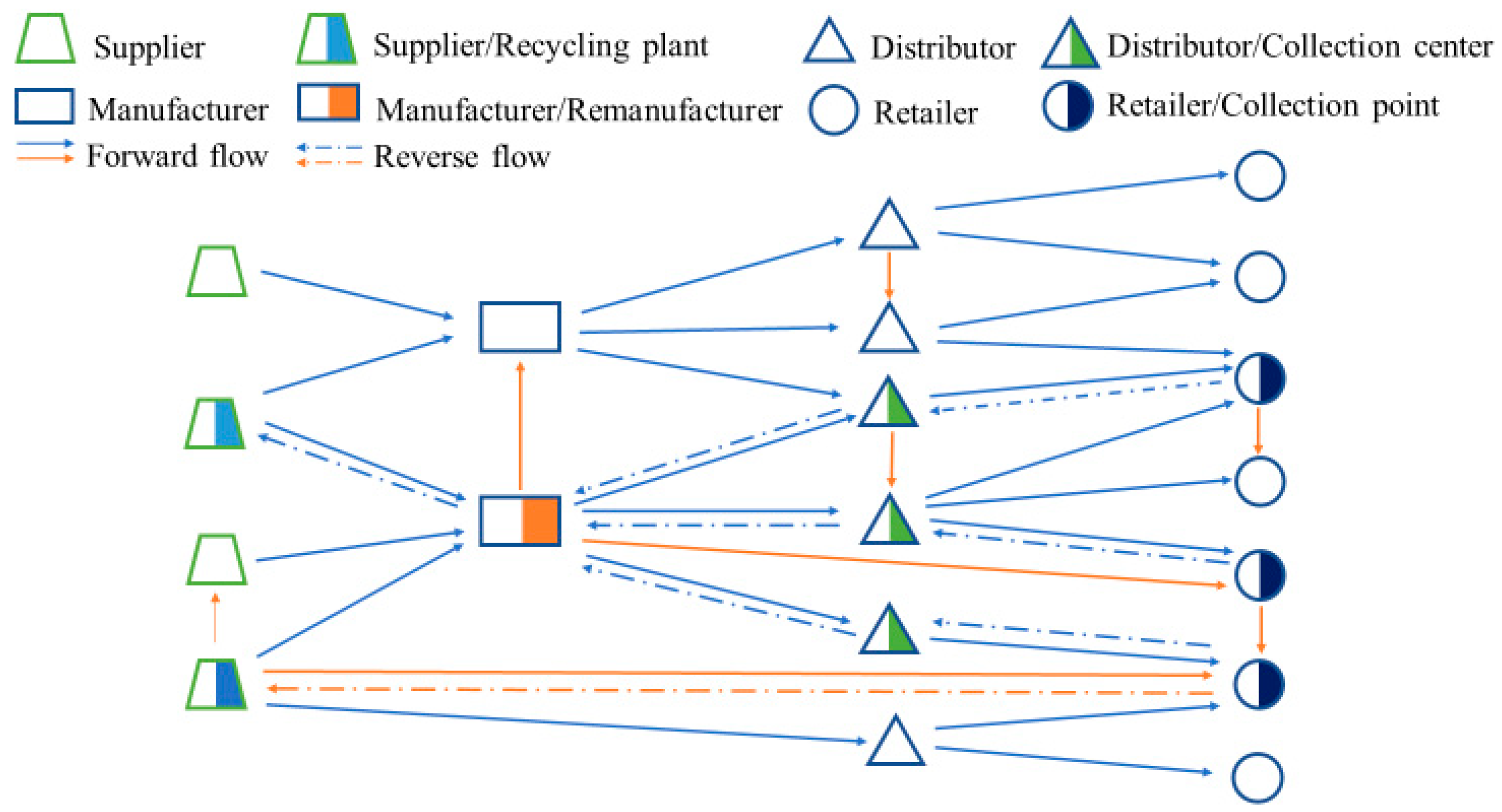
Figure 1 illustrates a CLSN, including 19 enterprises, 27 forward routes and 8 reverse routes. Traditionally, there are only vertical edges (blue edges); that is, the flow of raw materials and goods can only occur between upstream enterprises and downstream enterprises in the next tier, and this is a strict condition. However, with recent technological developments, there can be more complex links between enterprises than ever before. Therefore, horizontal edges (orange edges) are introduced into SNs [14], meaning that the goods and raw materials can be transported from manufacturer to manufacturer, from supplier to supplier, from manufacturer to retailer and so on.

With regard to the construction of CLSNs, the goal is usually to minimize costs or maximize profits. However, because of globalization and the increasingly complex division of labor, SNs are becoming increasingly complex and large. Due to the complex dynamic environment, random failures or targeted attacks occur frequently. Therefore, the robustness of SNs has drawn close scrutiny from researchers. Robustness is a proactive strategy that can be defined as the ability of an SN to resist change without adapting its initial stable configuration [15]. Namely, a robust supply chain endures, rather than responds, to changes. Change or uncertainty can refer to business-as-usual random variables [16,17], such as changes in raw material prices, energy consumption, market demand and labor costs, and extreme events such as natural disasters and political or military attacks, which may be unpredictable, but seriously harmful for the capabilities and operations of SNs [18].

For the problems of robust CLSN design, Pishvaee et al. [19] proposed a robust optimization model based on the extensions in robust optimization theory for coping with the inherent uncertainty of the input data. Considering uncertainty in the demand and the quantity of returned products simultaneously, Cui et al. [20] proposed a mixed-integer programming model with the aim of minimizing the total cost of CLSNs, and a novel, genetic, artificial bee colony algorithm was introduced to solve the model. Farrokh et al. [21] considered the CLSN design problem under hybrid uncertainty because of the inherent variability and unavailability of data in real environments, and a robust fuzzy stochastic programming approach was proposed. Except for the uncertainty due to the dynamic and turbulent nature of SNs, studies have indicated that catastrophic events can also be the sources of SN failures [22,23]. Therefore, Jabbarzadeh et al. [24] proposed a stochastic robust optimization model for the design of a CLSN that is resilient to random disruptions; the method can be utilized to minimize the total cost incurred across different disruption scenarios. Furthermore, Prakash et al. [25] formulated a mathematical model for CLSN design under simultaneous disruption risks and demand uncertainty, and then a case study was implemented to demonstrate the efficiency of the proposed model.

The present CLSN design problems, as noted above, mainly focus on the minimization of costs under uncertain conditions. The robustness of the CLSN is not the direct optimization target. The design processes often refer to the building of new facilities and the selection of their locations. However, in this paper, we assume a CLSN is built by adding new functions to the original facilities and choosing proper potential reverse routes based on the edges of the FSN, since the sharing of facilities and transportation routes can significantly enhance efficiency and save costs. In this situation, because of the limitations of objective conditions, such as having limited funds for constructing the reverse supply network or limited demand for reverse flow, it can be assumed that we should only establish a limited number of reverse routes to build a CLSN. Namely, it can be regarded as adding a certain number of reverse direction edges to the original SN. We concentrate on (1) if the different schemes of adding edges can influence the robustness against malicious attacks and (2) how to obtain the optimal scheme. Therefore, our optimization objective is to directly optimize the robustness of the designed CLSN from the macro perspective provided by network science. To achieve this, a robustness index is proposed as the fitness value, and then a multi-population evolutionary algorithm with novel operators is developed to find the optimal fitness value. At last, both the generated and realistic SNs are taken as examples to validate the effectiveness of our proposed method.

The sections below are organized as follows. Section 2 introduces a growth model to generate an FSN and the proposed robustness index for a CLSN. For robustness optimization, a multi-population evolutionary algorithm with novel operators is proposed in Section 3. Simulation results are illustrated and discussed in Section 4. The conclusion and future research ideas follow in Section 5.

2. Growth Model for SNs and the Robustness Index

To answer the aforementioned questions, we should first obtain an FSN. Many researchers utilize random graph and scale-free networks to study the robustness of networks against disruptions [26]. Perera et al. [27] systematically analyzed a set of SNs in the manufacturing sector to establish their topological characteristics and found that the degree distributions for the majority of the directed material flow networks indicated good fits with the power laws. Since scale-free networks have power law distributions for their degrees, an SN growth model based on a network model proposed by Barab’asi and Albert, known as the BA scale-free network model today, was utilized to generate an FSN [28,29], and it is described as follows:

Growth. We start with a fully connected network possessing $m_0$ nodes. At each time step, a new node is introduced to the existing network, and the new node is connected to m ($1\le m\le m_0$) old nodes simultaneously.

Preferential attachment. The probability that the abovementioned new node is connected to node i is shown in Equation (1):

$${\mathsf{\Pi }}_i=\frac{A_i}{{{\displaystyle \sum }}_{\forall k}{A}_k}$$

(1)

where $\forall k$ represents the summation that includes all old nodes and $A_i$ is defined in Equation (2) below:

$$A=\{\begin{array}{c}{m}_{0,}{D}_i\le m_0\\ \mu D_i^{\eta },D_i>m_0\end{array}$$

(2)

where D_i is the degree of node i and $\mu \left(\mu >0\right),\eta (\eta >0)$ are tunable parameters. Thus, after t steps, the total number of nodes is $N=m_0+t,t=0,1,2,\dots$ Because routes in SNs have directions, we randomly assign a direction to each edge of the generated networks.

In addition, since the degree distribution of an SN obeys the power law, assuming that the node degree distribution follows the power law if degree $D\ge D_{min}>0$, the power law exponent (scaling exponent) γ can be estimated as follows [30]:

$$\gamma =1+n{\left({{\displaystyle \sum }}_{i=1}^n\ln \frac{D_i}{D_{min}}\right)}^{-1}$$

(3)

where $D_i,i=1\dots n$ are the observed values of the degree such that $D\ge D_{min}$. In [27], it is stated that the real-world SNs indicate a value of γ in the range of 1–3. Gang et al. [31] researched the topological properties of an SN for agricultural products and found it to be scale-free, with an exponent $\gamma =2.75$. Therefore, we generated an FSN based on the aforementioned model with the following parameters: $m=m_0=2$, $N=500$, $\mu =2$ and $\eta =1$. Based on Equation (3), the value of γ for the generated FSN is 2.79, which is appropriate.

SN disruption is usually caused by two types of attacks [32]: random failures (e.g., natural disasters) and targeted attacks (e.g., political and military conflicts) [33]. Since these unexpected events contribute to an increase in SN complexity and vulnerability to disturbances, to survive, an SN must be robust [34]. There are many metrics for verifying SN resilience or robustness, and they are mainly based on concepts related to the largest connected component (LCC), such as the size of the LCC [35], the average path length in the LCC and the maximum path length in the LCC [36,37]. However, in previous studies, most network metrics were proposed to measure the robustness of FSNs. In this paper, we utilize the remaining edges in the LCC after attacks to measure the robustness $R$ of the CLSN as follows:

$$R=\frac{1}{101}{\displaystyle \sum }_{q=1}^{101}S\left(q\right)$$

(4)

where $S\left(q\right)$ is the fraction of directional edges in the LCC after removing Q nodes:

$$Q=0.01\times \left(q-1\right)\times N$$

(5)

Namely, during every iteration of an attack, we removed one percent of the nodes in the CLSN and calculated the ratio of the remaining directional edges in the LCC to the total edges in the original CLSN. The larger R was, the better the robustness of the CLSN would be.

3. Multi-Population Evolutionary Algorithm for Optimizing Robustness

The robustness of SNs can be analyzed and optimized from the perspective of complex networks [38], whose robustness is often optimized by evolutionary algorithms (EAs) [39]. Zhou and Liu [40] proposed a two-phase multi-objective EA to improve the robustness of networks against multiple malicious attacks. Qiu et al. [41] built a multi-population coevolution algorithm for the robustness optimization of wireless sensor networks characterized by scale-free topology. In turn, Yang and Liu [42] utilized an improved memetic algorithm to search for the optimal combination of removing the nodes with the lowest costs. With this algorithm, networks can be destroyed to the desired degree.

The most widely used branch of EAs is the genetic algorithm (GA). For instance, Ren et al. [43] utilized the multi-objective GA to optimize the robust adaptation of gene regulatory networks by searching the feasible topologies and the corresponding parameter sets. In [44], Ren et al. took advantage of a GA to design an integrated forward–reverse logistics network while accounting for carbon cap-and-trade considerations and total cost optimization.

Therefore, in this paper, a multi-population algorithm based on GAs with novel operators is proposed to find the transformation scheme with the optimal value of R when the CLSN is built based on an extant FSN, and this algorithm is abbreviated as MPEA-RSN. Since we assume that a limited number of reverse routes should be established to form a CLSN, $P_t$ is defined as the ratio of $E_r$ to $E$, where$E_r$ is the number of reverse edges (routes) in the established CLSN and $E$ is the number of edges in original FSN. Therefore, the optimization problem can be described as below:

$${\max }_{I}R\left(I\right)$$

(6)

$$s.t.\left|I\right|=E_r=\mathrm{Round}\left(E\times P_t\right)$$

(7)

where$I$ is the reverse route set selected to build along with the forward routes in an extant FSN and $R\left(I\right)$ represents the corresponding value of $R$. $\left|I\right|$ denotes the cardinality of $I$, and $\mathrm{Round}(·)$ is the nearest integer function.

3.1. Initialization

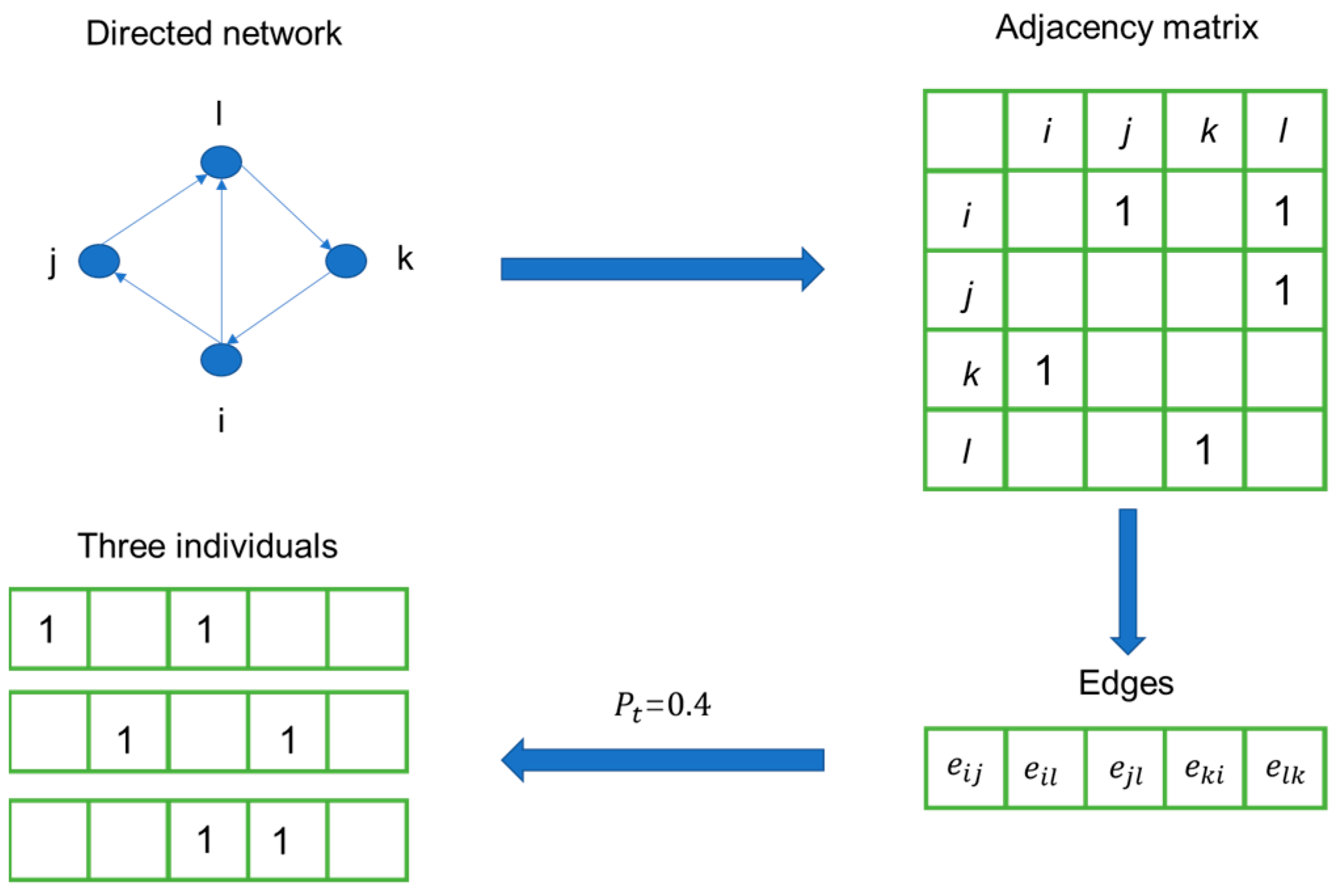
In the algorithm, we should generate individuals, each of which can exclusively represent a feasible solution. Namely, an individual can represent the reverse routes built along with the forward routes of the FSN to form a CLSN in this context. That is, a potential scheme for building a CLSN should be encoded into a binary-coded chromosome. Generally, a directed unweighted network can be represented by an adjacency matrix, which can be defined as an $N\times N$ constant matrix, and a 1 in the ijth entry indicates that node i and node j are connected. For example, if $N=500$, the FSN generated by the growth model can be denoted by a $500\times 500$ asymmetric matrix. In addition, the pairs of row and column indices $\left[ij\right]$ for all nonzero elements can be found, and the total index number equals the total edge number $E$ in the generated FSN. Therefore, we can generate a 0–1 string as an encoded individual with a length E, in which the element is 1 if we add another edge in the reverse direction at the corresponding location of a directed edge; the element is 0 otherwise. Based on the abovementioned constraints, there should be a fixed number of routes in the opposite direction added to the original FSN. Since a 1 in an individual indicates the location of reverse routes, the number of ones in an individual should equal the number of reverse routes. Therefore, there should be a fixed number of ones in each individual, which can be calculated by Equation (7).

An example is illustrated in Figure 2, where $e_{xy}$ ($x\ne y\wedge x,y\in \left\{i,j,k,l\right\}$) represents the edge from node x to node y. When $P_t=0.4$, a directed network with four nodes and five edges is converted into three individuals during the processing of initialization. Concretely, the number of ones in the adjacency matrix of the FSN is five. Therefore, the corresponding five routes (edges) in the FSN can be found and sorted based on the indices of the rows and columns. Since $E_r=\mathrm{Round}\left(5\times 0.4\right)=2$, we randomly selected two edges, and the reverse edges should be built at the corresponding locations. In this way, different individuals can represent different schemes for generating CLSNs.

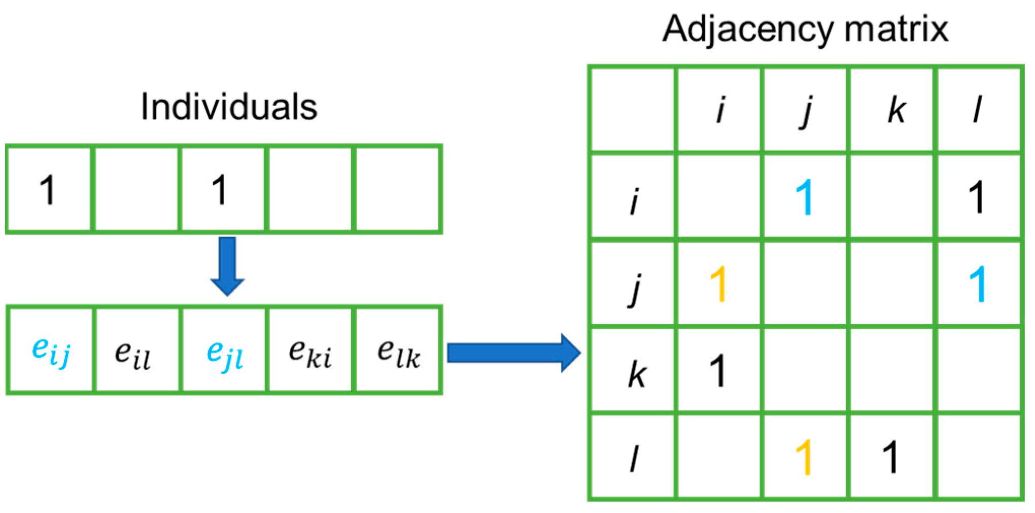
3.2. Decoding and Calculating Fitness

To calculate the fitness of individuals, we decoded an individual into an adjacency matrix that could represent a CLSN and then calculated the robustness of the network, which could be regarded as the fitness of the corresponding individual.

The process of generating the adjacency matrix of a CLSN is shown in Figure 3. As mentioned above, the ones in an individual can indicate the locations where the reverse routes are added into the original FSN. As shown in the adjacency matrix, the reverse edges should be added along with the edges represented by the ones in blue, and the orange ones, which represent added edges, should be diagonally symmetrical to the blue ones in the adjacency matrices of the CLSNs.

Once the generation of the corresponding adjacency matrices was completed, we could simulate node attacks on the CLSN and calculate the robustness $R$ based on Equation (4), which could be regarded as the fitness function in our algorithm.

3.3. Crossover and Mutation

The crossover operator was utilized to increase the size of the solution space and population diversity. After calculating the fitness of all individuals, the individuals were ranked according to the fitness values in descending order, and a certain number of individuals in the front were selected into the parent set. Any two individuals in the parent set, termed the father and mother, could be selected by the roulette wheel selection strategy [45] to generate the son and daughter. It is worth noting that the number of ones in each individual must remain unchanged after the crossover operation, since the number of ones in an individual indicates the number of reverse routes added, which is assumed to be fixed. To guarantee this, we adopted the following method.

Suppose the individuals $S_f$ and $S_m$ are the father and mother, respectively. Then, the calculations are performed as shown below:

$$L=S_f\cap S_m$$

(8)

$$U_f=S_f-L$$

(9)

$$U_m=S_m-L$$

(10)

L could represent the common locations where the reverse direction edges are added in the CLSNs represented by the father and mother. Equation (8) could be implemented by multiplying $S_f$ and $S_m$ element by element. Therefore, a one in $U_f$ in Equation (9) could denote the unique edges in the father that were not in the mother. Similarly, in Equation (10), $U_m$ denotes the unique edges in the mother. $U_f$ and $U_m$ have the same number of ones, but in different locations. We randomly generated an integer q that was smaller than the total number of ones in $U_f$ and $U_m$. The index of the qth one could be found as the breakpoint of $U_f$ and $U_m$, as shown in Figure 4, so we could obtain offspring as follows:

$$U_f=U_f^f+U_f^b$$

(11)

$$U_m=U_m^f+U_m^b$$

(12)

$$S_s=L+U_f^f+U_m^b$$

(13)

$$S_d=L+U_f^b+U_m^f$$

(14)

where $U_f$ or $U_m$ is divided by the breakpoint and $U_f^f$ or $U_m^f$ (including the breakpoint) is the front part of $U_f$ or $U_m$ after disconnection. Accordingly, $U_f^b$ or $U_m^b$ is the back part, and $S_s$ or $S_d$ is the son or daughter (i.e., the individuals generated after the crossover operation) [41]. In practice, $U_f^f$ or $U_m^f$ could be obtained by setting the ones after the breakpoint to 0; $U_f^b$ or $U_m^b$ could be obtained by setting the ones before the breakpoint (including the breakpoint) to 0. In this way, $U_f$ and $U_m$ contain different breakpoint locations, but we could guarantee that there were a fixed number of ones for each individual to satisfy the previously stated assumption. Finally, the generated offspring replaced the individuals not selected in the parent set.

For the mutation operator, on the premise of maintaining the number of nonzero elements, all individuals except the one with the best fitness value mutated, based on the mutation probability. For the mutation process, we randomly selected j ($j=1$, based on a large number of experiments for obtaining optimal results) pairs of zero elements and nonzero elements in an individual and switched their positions.

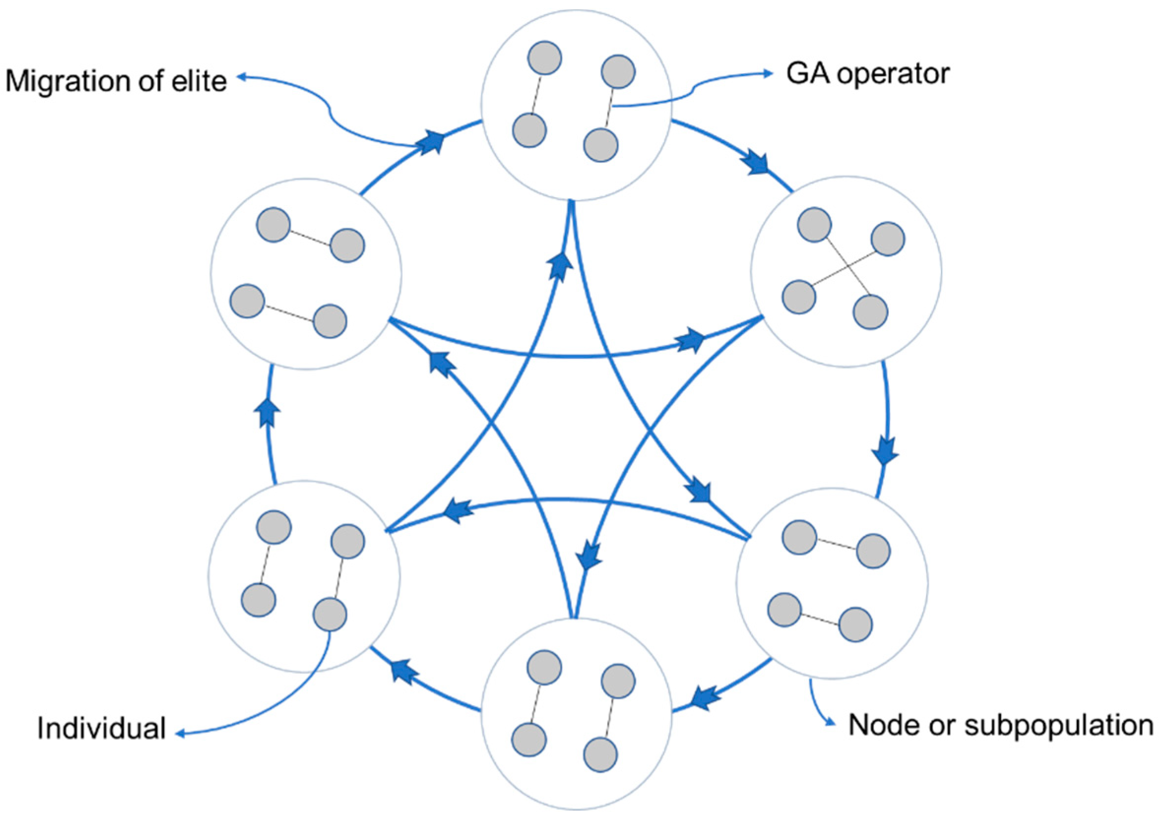
3.4. Migration

The multi-population strategy is universally utilized in EAs to maintain diversity and prevent premature convergence [46]. How the interaction structure of these subpopulations affects the performance of an EA has been discussed from the perspective of complex networks [47,48,49]. In this paper, we utilize the ring-shaped network as the topology of the communication structures of subpopulations. In this way, we can regard subpopulations as nodes and migrations between two subpopulations as edges, as shown in Figure 5.

During the migration process, after ranking again, one subpopulation receives two elite individuals from two nearby subpopulations to replace its worst two individuals. For instance, if we generate m ($m\ge 3$) subpopulations, the ith $\left(i\ge 3\right)$ subpopulation receives elites from the $\left(i-1\right)$ and $\left(i-2\right)$ subpopulations. Specifically, the second subpopulation receives elites from the first subpopulation and the mth subpopulation. The first subpopulation receives elites from the mth and (m − 1) subpopulations.

3.5. Implementation of MPEA-RSN

We first selected an FSN, which could be a network generated by the abovementioned growth model or a realistic SN, as the foundation for building a CLSN. Then, we initialized $M$ subpopulations with $S$ individuals in each of them, namely a total of $M\times S$ individuals. In each subpopulation, after ranking the individuals based on fitness by calculating R, the parent individuals with the best fitness values were selected to implement the crossover operation and generate offspring, which replaced the individuals not selected in the parent set. After subsequent mutation, the individuals of each subpopulation were ranked again, and elites migrated based on our migration strategy. The framework of MPEA-RSN is illustrated in Algorithm 1.

Algorithm 1 MPEA-RSN

Input:           $S{N}_0$: the original FSN;           $E$: the total edge number of S$N_0$;           $M$: the number of subpopulations;           $S:$ the size of each subpopulation;           $S_r$: the number of individuals that remain unchanged during the crossover operation;           $P_m$: the mutation probability;           $P_t$: the ratio of the number of reverse direction edges added to the FSN to $E$;           $f\left(x\right):$ the fitness function for calculating $R$; Output:           $R^{*}:$ the best fitness value;           ${\mathit{g}}^{*}$: the best individual found;

$G=\left\{G^1,G^2,\cdots G^M\right\}$ ← initialization ($S{N}_0$,$E$,$M$,$S$,$P_t$); $R$ ← $f\left(G\right)$; $G$ ← sort $\left(G\right)$ based on R; While (termination criteria are not satisfied) do             For i_sub = 1: $M$ do                 $G_c^{i\_sub}$ ← crossover ($G^{i\_sub}$, $S_r$);                 $G^{i\_sub}$ ← mutation ($G_c^{i\_sub}$,$P_m$);             End for             R ← $f\left(G\right)$;             $G$ ← sort $\left(G\right)$ based on R;             $G$ ← migration ($G$); End while Find the best individual ${\mathit{g}}^{*}$ from $\mathit{G}$ and the corresponding fitness value ${\mathit{R}}^{*}$.

4. Simulation Results

To obtain simulation results, we took the generated SN and a realistic SN as examples. The former was discussed in Section 2. The latter was abstracted from a supply chain of farm machinery and equipment and was composed of 76 suppliers, 30 manufacturers, 30 distributors, 570 retailors and a total of 908 links [50].

We simulated malicious attacks by removing the important nodes, and the importance of the nodes could be measured by node centrality (for example, degree centrality) [51]. In this paper, the betweenness centrality [52], which measures how often each node is located in the shortest path between all pairs of nodes, was employed to measure importance. Concretely, the betweenness of node u can be formulated as follows:

$$c\left(u\right)={\displaystyle \sum }_{s,t\ne u}\frac{n_{st}\left(u\right)}{N_{st}}$$

(15)

where $N_{st}$ is the number of shortest paths from node s to node t and $n_{st}\left(u\right)$ is the number of shortest paths from s to t that contain u. Therefore, the betweenness of each node in a CLSN was calculated first, and all nodes were then ranked in descending order, based on their betweenness values. By using this order, we implemented the process of removing nodes when calculating $R$ under malicious attacks.

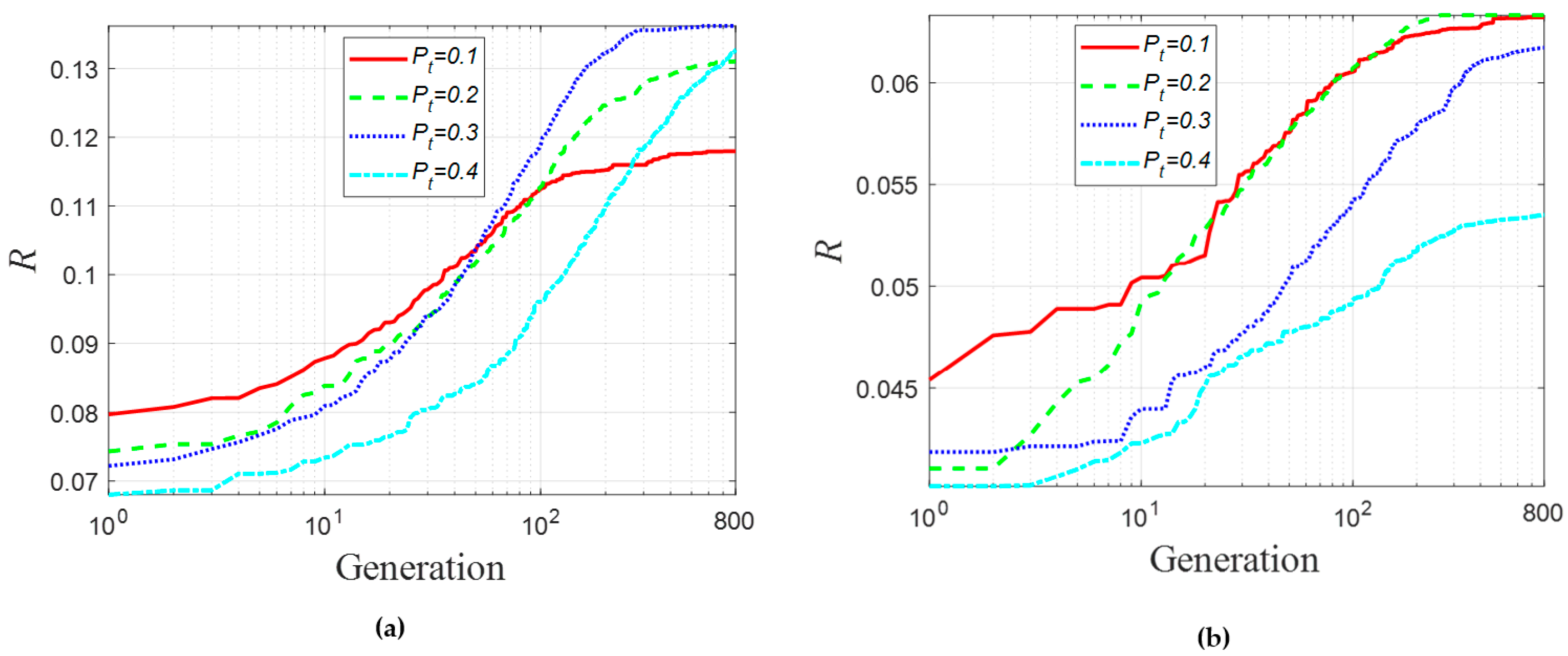
4.1. Optimization Results with Different Values of $P_t$

In this subsection, we employ the MPEA-RSN algorithm to optimize the two specific examples to obtain more robust results when transforming the FSN into a CLSN. After numerous trials, the parameters of the simulation (set as follows) were thought to be appropriate: $M=8,S=60,S_r=40$ and $P_m=0.9$. The value of $P_t$ increased from 0.1 to 0.4, and the interval was 0.1. Figure 6 illustrates the best simulation results obtained by the algorithm after repeated runs.

In Figure 6a, the initial topologies of the CLSNs are initialized based on the generated SN, and lines show the variation in R over all iterations. The X-axis represents the number of generations, and the Y-axis represents the value of R, indicating the robustness of the CLSN to malicious attacks. As the number of generations increased, the value of R showed an upward trend for each line, which indicates the effectiveness of MPEA-RSN in optimizing CLSNs. Finally, the proportions of the increased robustness values to the original robustness values were $48.0\%,$ $76.4\%$, $88.6\%$ and $95.1\%$ for $P_t=0.1,0.2,0.3,0.4$, respectively. It is noted that as $P_t$ increased, the effect of optimization became more significant.

Similarly, in Figure 6b, the topology of the abovementioned realistic SN is chosen as the foundation network, and the variation in R is displayed. The proportions of the increased robustness values to the original robustness values were $39.2\%,$ $54.2\%,$ $47.4\%$ and $33.3\%$. For the realistic network with a larger scale than the generated one, as $P_t$ increased, the effect of MPEA-RSN in terms of optimizing CLSNs first improved, but then deteriorated. Besides that, when $P_t=0.4$, the value of $R$ after optimization became much lower than other optimized values of $R$, indicating a proper value of $P_t$ should not be too large for the realistic SN taken as an example.

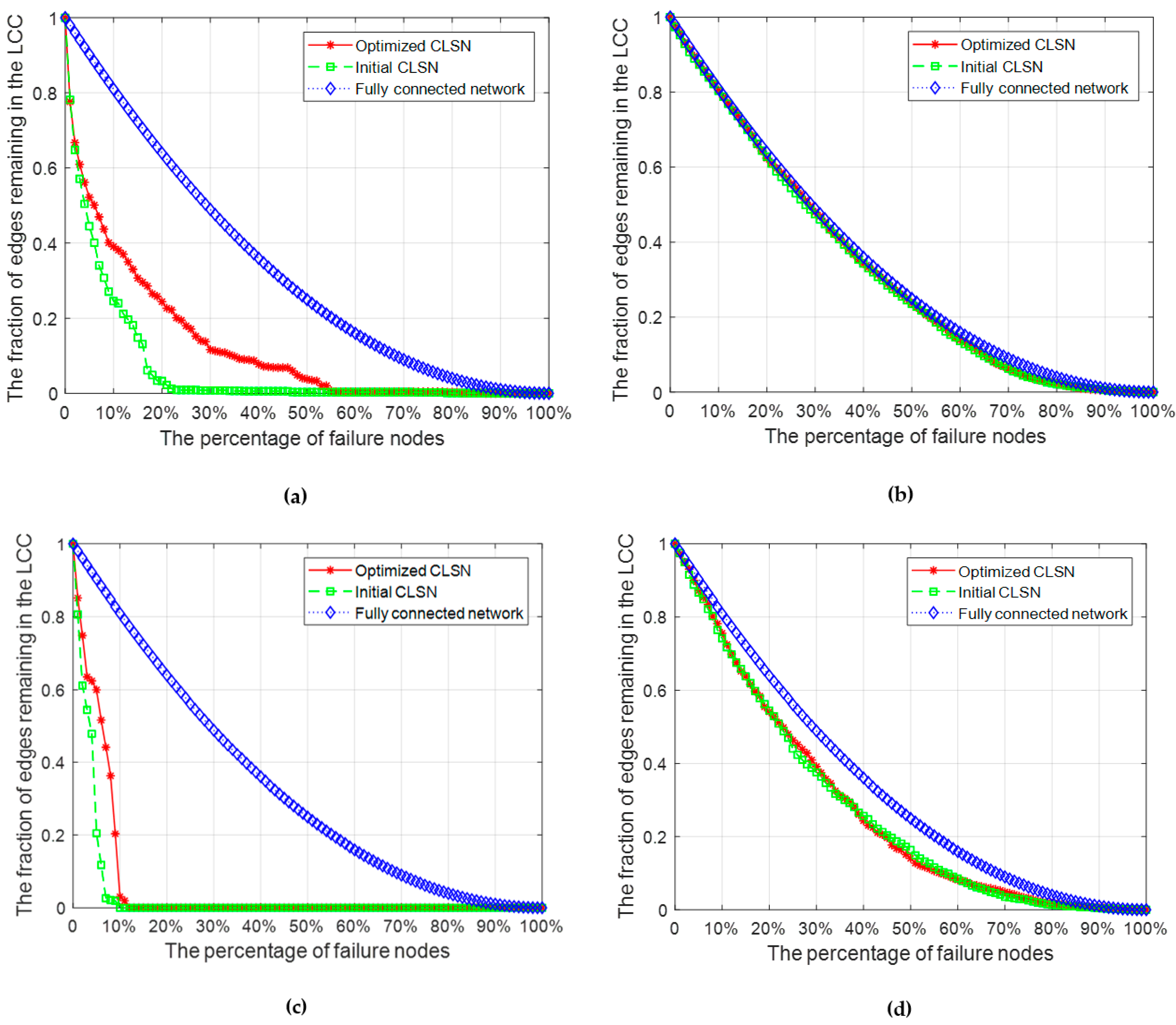
4.2. Comparison of Robustness before and after Applying the MPEA-RSN Algorithm

To further observe the increase in robustness after optimization, the initial randomly generated CLSN and the CLSN after optimization by MPEA-RSN were compared by measuring the fraction of edges remaining in the LCC after removing a certain percentage of nodes. As shown in Figure 7, the green line denotes the initial CLSN, and the red line denotes the optimized CLSN. In addition, the blue line represents the fully connected network as a frame of reference in which, between every pair of nodes, there exist two directed edges in the reverse direction to connect them.

Figure 7a,c simulates the CLSNs under malicious attacks. The X-axis represents the percentage of failure nodes, and the Y-axis represents the fraction of edges in the LCC. In both figures, the red lines are basically above the blue lines and close to the blue lines, which means that the optimized CSLNs had better robustness than the initial CLSNs.

As shown in Figure 7b,d, the robustness of the CLSNs against random attacks was studied. We simulated this type of attack by removing nodes randomly, rather than specifically removing important nodes. Since the random attacks were stochastic, we simulated the process 20 times and calculated the average of the obtained values. The red line and green line are basically consistent, indicating that optimizing the robustness of the network against malicious attacks did not destroy the ability of the CLSN to resist random attacks.

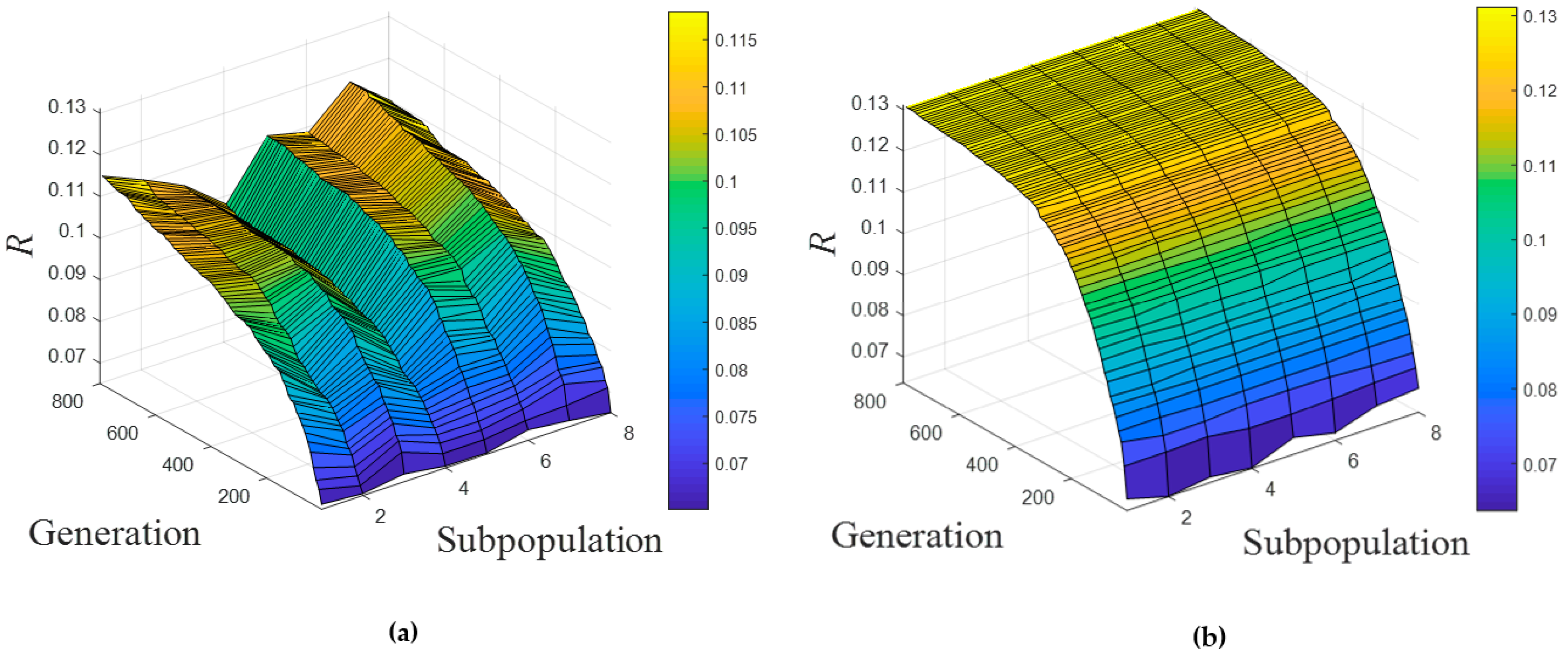
4.3. Comparison between the Conventional GA and the MPEA-RSN Algorithm

In this section, we compare our proposed algorithm to the conventional GA. To intuitively observe the effects of the different algorithms, we ran the conventional GA on eight independent populations simultaneously for optimization purposes, while the subpopulation number for MPEA-RSN was also eight. Both the crossover and mutation operators were completely the same, except that there existed no migration between populations in the conventional GA. The parameters in both algorithms were set as follows: $S=30,S_r=20,P_m=0.9$ and $S{N}_0$ is the generated network.

Figure 8a shows the best fitness values of the eight independent populations in each generation, along with their evolution. The results were very different, and premature convergence occurred very early in some populations, so the optimal value could not reach a high level compared with that of the MPEA-RSN algorithm, as shown in Figure 8b. Given that migration operations can introduce excellent individuals to other subpopulations, the fitness value can avoid falling into the local optimum too early and obtain a superior optimum. Figure 8b also illustrates the effectiveness of the proposed algorithm to optimize the robustness of CLSNs. Concretely, the robustness of the initial CLSN was low, and the increase in $R$ was obvious in the beginning. After approximately the 300th generation, the optimization result improved slowly because the value of $R$ had increased to a high level.

4.4. Discussion and Results Analysis

The simulation results illustrated in Figure 6 demonstrate the effectiveness of MPEA-RSN, indicating that the different schemes for adding reverse routes to an FSN could lead to different robustness values. With the variation of the $P_t$ value, the optimized values of $R$ were variable, too. Furthermore, the proportions of the increased robustness values to the original robustness values were significantly different. Namely, the optimization effect was also changed with the variation of the $P_t$ value. For the generated and realistic SNs, the most significant effect appeared at different values of $P_t$, indicating the effect of optimization by MPEA-RSN could be significantly impacted by the structural characteristics of the original SNs. Not only does Figure 7 indicate that the optimization processes did not destroy the ability of the CLSNs to resist random attacks, but the faster decrease of the corresponding curves for malicious attacks indicates that the CLSNs built based on the generated or realistic SN were more vulnerable to targeted attacks than random attacks, though the robustness against malicious attacks had been optimized. This can also indicate that there are a small number of highly connected hub nodes and a high number of feebly connected nodes in SNs [32].

5. Conclusions and Future Scope

How to build robust CLSNs against malicious attacks based on extant FSNs has hardly been discussed before, especially from a macro perspective which can be provided by network science. Therefore, we first introduced the index R to measure the robustness of CLSNs, and then we proposed a coevolution algorithm called MPEA-RSN to optimize the transformation schemes. In the algorithm, the encoding and decoding were designed based on the characteristics of the problem. Then, a crossover operator with different breakpoints for parent individuals was proposed to guarantee that the number of ones in each binary individual remained unchanged due to problem-based constraints. At last, a generated SN based on the growth model and a realistic SN were taken as examples to validate the effectiveness of our proposed algorithm. The simulation results showed that the robustness of CLSNs built against malicious attacks could be optimized by our algorithm, while the robustness against random attacks remained almost unchanged during optimization. The best experimental results show that the robustness of the CLSN can be nearly doubled ($95.1\%$). Therefore, when managers plan to build a CLSN, MPEA-RSN can be utilized to theoretically find the most robust schemes against malicious attacks and provide a frame of reference for the choice of the $P_t$ value from a robustness perspective.

In our network model, the heterogeneous attributes of nodes are not considered. However, the fact that the nodes in an SN have different roles or functions has attracted the attention of researchers, and this can be taken into account in future work when we characterize the robustness of SNs. In addition, the effect of a malicious attack is static in this paper, and cascading failure is not considered, so the spreading of failed loads may also be considered in future work.