Investigation of Electrochemical Processes in Solid Oxide Fuel Cells by Modified Levenberg–Marquardt Algorithm: A New Automatic Update Limit Strategy

Abstract

Identification of ongoing processes in solid oxide fuel cells (SOFC) enables both optimizing the operating environment and prolonging the lifetime of SOFC. The Levenberg–Marquardt algorithm (LMA) is commonly used in the characterization of unknown electrochemical processes within SOFC by extracting equivalent electrical circuit (EEC) parameter values from electrochemical impedance spectroscopy (EIS) data. LMA is an iteration optimization algorithm regularly applied to solve complex nonlinear least square (CNLS) problems. The LMA convergence can be boosted by the application of an ordinary limit strategy, which avoids the occurrence of off-limit values during the fit. However, to additionally improve LMA descent properties and to discard the problem of a poor initial parameters choice, it is necessary to modify the ordinary limit strategy. In this work, we designed a new automatic update (i.e., adaptive) limit strategy whose purpose is to reduce the impact of a poor initial parameter choice. Consequently, the adaptive limit strategy was embedded in a newly developed EIS fitting engine. To demonstrate that the new adaptive (vs. ordinary) limit strategy is superior, we used it to solve several CNLS problems. The applicability of the adaptive limit strategy was also validated by analyzing experimental EIS data collected by using industrial-scale SOFCs.

1. Introduction

Electrochemical power sources, e.g., solid oxide fuel cells (SOFC) [1], are gaining an increasing interest due to new generation of SOFC devices that are more environmentally-friendly and highly-efficient. Nevertheless, there are still some issues with these devices (e.g., undesired degradation processes) that have to be detected at an early stage of their use. When employing appropriate diagnostic tools, degradation can be limited or even prevented, thus prolonging the SOFC lifetime. Electrochemical impedance spectroscopy (EIS) is an appropriate technique for examination of the aforementioned processes and could therefore be of crucial importance for this specific branch of industry. One should be aware of the fact, though, that since EIS works with a large amount of information, it is necessary to constantly develop new software/algorithms for EIS data analysis (e.g., [2,3]).

Numerous electrochemical processes that take place in SOFC can be characterized by EIS and examined in more detail by using diagnostic tools such as electrical equivalent circuit(s) (EEC) [4], the distribution of relaxation times [3,5] (DRT), and the distribution of diffusion times [6,7] (DDT). The EEC approach demands a specification of the EEC model, an initial parameters choice [8], and a selection of the appropriate optimization algorithm [9]. When investigating electrochemical processes in SOFC by using EEC, the initial parameter choice is one of the most important steps since it impacts the accuracy of the final result.

EEC parameters of electrochemical processes can be extracted by using diverse iterative algorithms [10]. Two optimization algorithms [11] that are relevant for EIS study are Levenberg–Marquardt [8,12,13,14] (LMA) and Nelder–Mead [15,16,17,18,19] (NMA). It is important to note that the majority of EIS data fitting software tools [8] applies LMA on account of its good convergence properties [8,20,21]. On the other hand, NMA does not require the first derivatives; and thus, it is a proper tool to fit noisy EIS data.

One of the greatest LMA drawbacks is the possibility of getting stuck in the local mathematical landscape of the complex nonlinear least-square (CNLS) problems [15,20]. This LMA weakness is rapidly intensified if a poor starting parameter choice is applied at the iteration start. In view of these matters, several studies have tried to improve LMA convergence properties by the application of a more advanced damping (λ) parameter strategy [8,22,23,24], and/or by using the ordinary limit strategy [20].

In our previous studies [20,21], the ordinary limit strategy [25,26] was successfully used to boost the LMA convergence. The aforementioned boost was gained by discarding off-limit values during the fit. This was accomplished by using a wide limit gap, which is defined by upper and lower limit bounds [20]. However, a large limit gap might intensify the problem of the starting parameters choice; and thus, the limit gap should be automatically adapted during the iterations.

In this work, a novel automatic update limit strategy that automatically adapts the limit gap during the LMA iteration process was designed. Furthermore, both the objective function and LMA that were applied in this study were briefly discussed. Finally, the new strategy was tested by the SOFC experimental EIS data to show its applicability.

The aim of this study was to (i) design a new adaptive limit strategy, (ii) boost the convergence properties of an LMA-based fitting engine, and (iii) conduct several tests by using both synthetic and the SOFC experimental EIS data.

Overall, the greatest contribution of this study is a design of the adaptive limits strategy that additionally discards a problem of poor parameter choice when using LMA to extract EEC parameter values of electrochemical processes under study.

2. Theory and Computations

2.1. EEC and Objective Function Used in EIS Study

One of the simplest electrical equivalent circuit (EEC) models (i.e., Randles circuit [4]) used for the EIS data fitting can be formulated as follows:

$$f\left({\omega }_i, a\right)={\mathrm{a}}_0+\frac{1}{\frac{1}{{\mathrm{a}}_1}+j{\omega }_i{\mathrm{a}}_2}=R_s+\frac{1}{\frac{1}{R_1}+j{\omega }_i{C}_1}; a=\left({\mathrm{a}}_0,{\mathrm{a}}_1,{\mathrm{a}}_2\right),$$

(1)

where $a, j, {\omega }_i$ are EEC parameters, the imaginary unit and the ith value of the angular frequency.

In order to extract EEC parameter values from, e.g., (1), the following objective function (see [27]) was used herein:

$$S=\frac{1}{m-r-1}\cdot {\displaystyle \sum }_{i=1}^m\left(w_i{\left(\mathrm{Re}\left(y_i^{exp}\right)-\mathrm{Re}\left(y_i^{com}\right)\right)}^2+w_i{\left(\mathrm{Im}\left(y_i^{exp}\right)-\mathrm{Im}\left(y_i^{com}\right)\right)}^2\right),$$

(2)

$$w_i=\frac{1}{\mathrm{Re}{\left(y_i^{exp}\right)}^2+\mathrm{Im} {\left(y_i^{exp}\right)}^2}$$

(3)

where $m,r, y_i^{exp}, y_i^{com} \mathrm{and}{w}_i$ are the number of data points, the number of EEC parameters, the ith value of experimental impedance data, the ith value of computed impedance data by EEC model (e.g., (1)) and the “weighting” modulus [28] factor associated with the ith data point, respectively. Moreover, to extract EEC parameters from EIS data, by using (2), it is common to use the Levenberg–Marquardt algorithm.

2.2. Optimization Algorithm Used in This Study

Data fitting is an optimization problem [9,11] which minimizes the quadratic objective function (2) by usually applying the Levenberg–Marquardt [12,13] algorithm (LMA). LMA is an iterative algorithm (see Algorithm 1) in which the following formulation is being repetitively solved in each iteration (∘ stands for element-wise multiplication):

$$h={\left(J^T\left(W\circ J\right)+\lambda I\right)}^{-1}\left(J^T\left(w\circ \left(y^{\exp }-y^{\mathrm{com}}\right)\right)\right),$$

(4)

where h, J, w, W, I, y^exp, y^com, and $\lambda$ represent the vector of computed increments in EEC parameters, the Jacobian matrix, the vector containing weights (3), the matrix with columns equal to vector of weights w, the identity matrix, the vector of experimental EIS values, the vector of computed EIS values, and the damping parameter.

Each LMA iteration is evaluated by using the gain factor ($\rho$) value:

$$\rho =\frac{S\left(a\right)-S\left(a+h\right)}{h^T\left(\mathsf{\lambda }h+J^T\left(w\circ \left(y^{\exp }-y^{\mathrm{com}}\right)\right)\right)},$$

(5)

where a is the vector of EEC parameters that define the values of y^com.

If $\rho >0$, then the iteration is successful, λ is decreased (see Algorithm 1), and the vector h is added to the parameter values ($a^t$) from the previous iteration (t):

$$a^{t+1}=a^t+h.$$

(6)

Otherwise, if $\rho \le 0$, then a^t is not updated and λ is increased (see Algorithm 1). The change in the λ value allows LMA to balance between the Gauss–Newton method (when near the solution) and the steepest descent (when far from the solution) [23,24]. For a more comprehensive study related to the $\lambda$ update strategy, the reader is encouraged to inspect the following papers [10,22,23,24].

Additionally, extracting EEC parameters from EIS data is an overdetermined nonlinear problem [9]; and hence, there are no exact solutions. This indicates that negative and off-limits EEC values can be generated during the fit [20] and they can be avoided by using the limit strategy.

Algorithm 1. Pseudocode of Levenberg–Marquardt algorithm (adapted from [22,24]). Symbol references: J is the Jacobian matrix, JT(W$\circ$J) is the approximate Hessian matrix; I is the identity matrix, JT(w$\circ$ (yexp − ycom)) is the gradient vector, w is the vector containing weights (3), and W is the matrix with columns equal to weights (3).

Levenberg–Marquardt algorithm

a = a0; λ = λ0; ν = 2

repeat

Solve (JT(W∘J) + λI)h = JT(w $\circ$ (yexp − ycom))

if ρ > 0

a = a + h

λ = λ ∗ max(1/3, 1 − (2ρ − 1)3)

ν = 2

else

λ = λ ∗ ν

end if

until

2.3. Limit Strategy in EIS Study

LMA is an unconstrained optimization algorithm as it applies the first derivatives [9]; and thus, it cannot handle limits in a straightforward manner. Nevertheless, the aforementioned problem was solved by integrating the ordinary limit strategy with LMA [20] (

Table 1. Limit strategies coupled with Levenberg–Marquardt algorithm in EIS study.

Limit Strategy	Automatic Limits Update	Reported in EIS
No limit	No	e.g., [8]
Ordinary	No	[20]
Automatic update (i.e., adaptive)	Yes	This work

). Furthermore, if the fitted values are too close to the lower or upper limits values, an additional numerical inaccuracy can occur [25,26]. In our previous studies [20,21], these limit values (see (9)) were predetermined prior to fitting. Therefore, herein we propose a new automatic update limit strategy that automatically adapts limit values during the iterations. The following sections present both the ordinary and adaptive strategies in more detail.

2.4. Ordinary Limit Strategy for Levenberg–Marquardt Algorithm

In order to use limits and to minimize the objective functions like (2), James et al. [25,26] proposed an approach which converts the starting (i.e., external) parameter values into the internal parameter values that are used during the fit:

$$a_{int,j}=k\left(a_{ext,j}\right)=\arcsin \left(2\frac{a_{ext,j}-l{b}_j}{u{b}_j-l{b}_j}-1\right),$$

(7)

$$a_{ext,j}=l\left(a_{int,j}\right)=l{b}_j+\frac{u{b}_j-l{b}_j}{2}\left(\sin a_{int,j}+1\right),$$

(8)

where a_int,j, a_ext,j, lb_j, and ub_j are the jth value of the internal parameter, the jth value of the external parameter, and jth values of lower and upper limits, respectively. The limit values are computed by:

$$l{b}_j= \frac{1}{{10}^{+5}}\left|a_{ext,j}\right|, u{b}_j= {10}^{+5}\left|a_{ex{t}_j}\right|,$$

(9)

where 10⁺⁵ is the limit update factor (LUF) that is given a priori. Only in the case of the parameter n, the limit values are set to 0.449 and 0.999.

Furthermore, at the beginning of the fitting process, a_ext,j is converted (7) into a_int,j (Algorithm 2). However, prior to each EEC model evaluation, a_int,j is converted back into a_ext,j. According to (8), a_ext,j can take on only the value from a limit gap which is characterized by lb_j and ub_j. To rephrase it, the EEC parameters can only have values from a specific and limited region. On the other hand, during the iterations, a_int,j can take on any value from the feasible solution space. Knowing this, the limit gap can also be taken into account as, e.g., a trust region, which is a term commonly used in the trust-region methods [9]. Since the size of this limit gap remains fixed during the whole iteration procedure, we refer to this strategy as the ordinary limit strategy (see Table 1).

Algorithm 2. Pseudocode of Levenberg–Marquardt algorithm, which is coupled by the ordinary limit strategy. Symbol references: J is the Jacobian matrix, JT(W∘J) is the approximate Hessian matrix; I is the identity matrix, JT(w$\circ$ (yexp − ycom)) is the gradient vector, w is the vector containing weights (3), and W is the matrix with columns equal to weights (3).

Ordinary limit strategy for the Levenberg-Marquardt algorithm

aext := a0; λ := λ0; ν := 2

aint := k(aext) (convert to aint by (7))

LUF := 1e5 (limits update factor)

compute limits ((7),(8),(9))

repeat

Solve (JT(W$\circ$J) + λI)h = JT(w $\circ$ (yexp − ycom))  (only here use l(aint) (8) instead of aint)

if ρ > 0

aint := aint + h

λ := λ ∗ max(1/3, 1 – (2ρ – 1)3)

ν := 2

else

λ := λ * ν

ν := ν * 2

end if

until

aext := l(aint) (convert to aext by (8) )

2.5. Automatic Update (i.e., Adaptive) Limit Strategy for Levenberg–Marquardt Algorithm

In order to resolve the numerical inaccuracy that occurs when EEC parameters are too close to the limit values we proposed an adaptive strategy that aims to keep these parameters within the limits by constantly monitoring the algorithm’s progress and adjusting the limits accordingly. This strategy decreases the limit gap when it detects that LMA starts to converge (Scheme 1). On the other hand, if the LMA becomes stuck, the adaptive strategy automatically increases the limit gap. The aforementioned approach is opposite to the one used by the trust-region methods [9].

Furthermore, to automatically tune the limit gap, the proposed automatic update limit strategy monitors the number of successive good (g) and bad (b) iterations (Algorithm 3). This is to ensure that the limit values are updated only in two cases. In the first case (g > 2), the LUF value (9) is decreased by factor 0.9, and limit values are recomputed (see Algorithm 3). In the second case (b > 2), the LUF value is increased by factor 2 and the limit values are again recalculated. According to [25], the aforementioned actions decrease a numerical inaccuracy. Note that both 0.9 and 2 values were selected during the experiments. Moreover, we tried several values and we detected that the rapid change in LUF can have a negative impact on the convergence; and thus, the sudden variation in LUF was avoided by using 0.9 and 2.

Algorithm 3. Pseudocode of the Levenberg–Marquardt algorithm, which is coupled by the automatic update limit strategy (see sub procedure). Symbol references: J is the Jacobian matrix, JT(W$\circ$J) is the approximate Hessian matrix; I is the identity matrix, JT(w $\circ$ (yexp − ycom)) is the gradient vector, w is the vector containing weights (3), and W is the matrix with columns equal to weights (3).
Automatic update limit strategy for the Levenberg-Marquardt algorithm
aext := a0; λ := λ0; ν := 2
g := 0; b :=0 (g and b are number of good and bad iterations)
LUF := 1e5 (limits update factor)
compute limits ((7),(8),(9))
aint: = k(aext)   (convert to aint by (7)))	sub update_limits
repeat	if g > 2
Solve (JT(W$\circ$J) + λI)h = JT(w $\circ$ (yexp − ycom)) (use l(aint) (8) instead of aint)	LUF := LUF*0.95; 10 ≤ LUF ≤ 104
if ρ > 0 (good iteration)	aext := l(aint)
aint := aint + h	compute lbi and ubi by aext,i
update_limits (using current l(aint) value)	compute aint,i:= k(aext,i) by new lbi, ubi
λ := λ ∗ max(1/3, 1 – (2ρ – 1)3)	end if
ν := 2	if b > 2
g := g+1; b := 0	LUF := LUF*2; 10 ≤ LUF ≤ 104
else  (bad iteration)	aext := l(aint)
λ := λ * 2	compute lbi and ubi by aext,i
ν := ν * 2	compute aint,i:= k(aext,i) by new lbi,ubi
g := 0; b := b+1	end if
end if	end sub
until
a := l(aint) (convert to aext by (8))

Furthermore, LUF values were limited between 10 and 10⁴ in order to allow both a sufficiently wide gap for convergence and to prevent an increase in the numerical inaccuracy. Please note that values 10 and 10⁴ used herein were selected during the testing, and their choice is not additionally explained.

To summarize, the proposed automatic limit update strategy is the opposite tactic to the one applied in the trust-region methods since the limit gap is being decreased during the convergence in order to additionally reduce the possibility of off-limit values during the fit.

3. Experimental

3.1. Synthetic Noisy ZARC Data Used in This Study

The synthetic ZARC data in this work were prepared by simulating three electrochemical processes using three ZARC elements (one for each process) and this was done by applying the following formulation:

$$R_s+{\displaystyle \sum }_{k=1}^{p=3}\frac{R_k}{1+{\left(j{\omega }_i{\tau }_k\right)}^{n_k}},$$

(10)

where R, ${\omega }_i,$ ${\tau }_k$, n_k, and p are resistances, the angular frequency associated with ith data point, the time constant associated with the kth ZARC process, the parameter associated with the τ distribution of associated kth ZARC process, and the number of ZARCs processes. The data were prepared by using 10 data points per decade. The EEC parameters used for ZARC data generation are given in

Table 2. EEC parameter values used to compute the synthetic ZARC data (10) in this work. Values in parentheses present τ values used to prepare ZARC data with a more corrupted local landscape.

EEC Parameters		EEC Parameter Values
		k
		1	2	3
Rs (Ω cm2)	10	-	-	-
Rk (Ω cm2)	-	50	50	50
τk (s)	-	0.01 (0.01)	0.001 (0.005)	0.0001 (0.001)
nk	-	0.7	0.7	0.7

.

With the intention of devising a more comprehensive study, ZARC (Z_ZARC) data were polluted by noise:

$$Z_{ZARC\_poll}\left(\omega \right)=Z_{ZARC}\left(\omega \right)·\left(1+0.005\cdot \left({\eta }^{\prime }+j{\eta }^{″}\right)\right),$$

(11)

where η′ and η″ are two independent normally distributed (Generated by numpy.rand.normal routine.) variables with zero mean and the unit variance, respectively. The usage of the constant factor of 0.005 produces at least 0.5% noise, but normally distributed noise (${\eta }^{\prime } \mathrm{and} {\eta }^{″}$) can take on arbitrarily large values. As LMA applies the first derivatives, the algorithm is sensitive to noise (see, e.g., [9,11]). As a result, by adding the noise, we can additionally test the convergence properties.

3.2. Experimental SOFC Data Used in This Study

The experimental EIS data were obtained by using industrial size solid oxide fuel cells (SOFC). The electrochemically active area of the cells was 80 cm². The cells were operated with different synthetic fuels (H₂ and CO, CO₂, CH₄, H₂O, and N₂) that have the same composition as gasses from biomass gasification. Such complex composition of the fuel results in numerous electrochemical processes, such as hydrogen oxidation, carbon monoxide oxidation, water gas shift reaction, steam and dry reforming, and many others. In order to investigate the processes within the fuel cell, we collected EIS data in the relevant frequency range from 0.1 Hz to 10 kHz.

Please note that due to both different gas compositions and the complexity of the reactions that can take place in parallel, several serial QR elements can be applied in the EEC model. These QR elements are usually used to simulate the porous electrodes’ structure, thus referring to different chemical and electrochemical processes that can occur. It has to be mentioned that slight nonlinearities in the low-frequency range are expected due to the ongoing reactions and varying amount of steam.

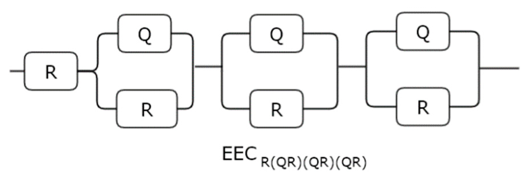
3.3. EEC Model Used in This Study

Herein, the EEC_{R(QR)(QR)(QR)} model was applied that is a serial combination of three (k = 3) parallel QR elements (Figure 1). The model is characterized by three time constants, i.e., by the same number of time-constants that describe ZARC processes in this work (Table 2). Next, the EEC_{R(QR)(QR)(QR)} model in Figure 1 can be represented by:

$$R_s+{\displaystyle \sum }_{k=1}^{p=3} \frac{1}{\frac{1}{R_k}+Y_{0,k}{\left(j\omega \right)}^{n_k}},$$

(12)

where, $R,p, Y_0 and n$ represent resistances, total number of serial circuits, coefficient related to constant phase element (Q), and parameter related to the τ distribution.

EEC_{R(QR)(QR)(QR)} parameter values used to start fits in this study are presented in

Table 3. The starting values of the EEC_{R(QR)(QR)(QR)} parameters used to initiate the fits in this work. The values in parentheses represent poor starting values taken by design to be far from the optimal values.

EEC Parameters		EEC Parameter Values
		k
		1	2	3
Rs (Ω cm2)	10 (1.1)	-	-	-
Y0,k (S sn cm−2)	-	0.1 (1.2)	0.01 (1.3)	0.001 (1.4)
nk	-	0.85 (0.85)	0.83 (0.83)	0.87 (0.87)
Rk (Ω cm2)	-	70 (1.5)	20 (1.6)	50 (1.7)

. Two types of starting parameter values were used herein. First, a good starting guess (chosen close to the optimal values), which is typical in EIS study, especially as the starting values are vital when commencing LMA fit [8,20] and second, a poor starting guess that was taken by design to be far from the solution to show the robustness gained by the application of the automatic limit update strategy.

3.4. Open-Source Packages Used in This Study

The Python v3.7.4 programming language was used herein and the following open-source Python modules were applied:

-

NumPy [29] v1.17.2.

-

Matplotlib [30] v3.1.3.

4. Results and Discussion

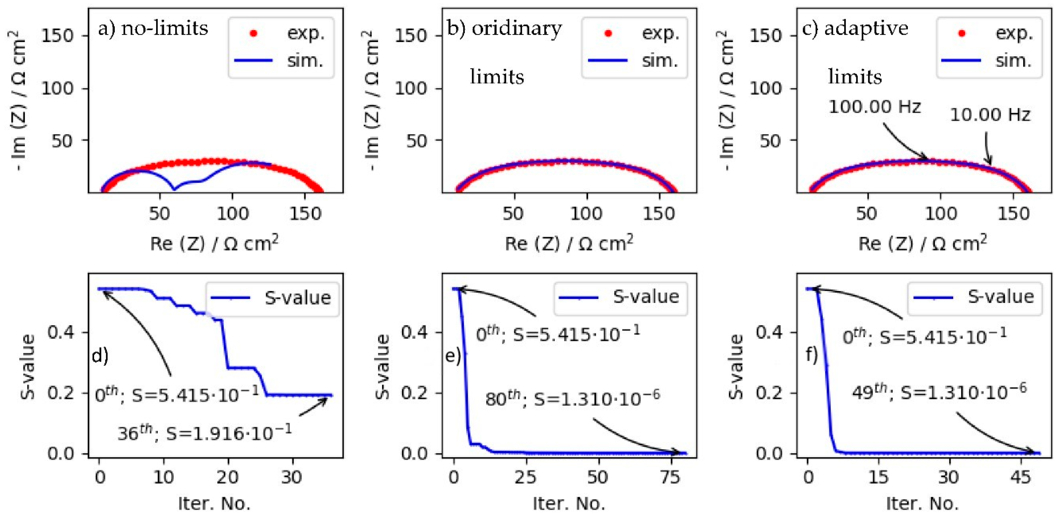
4.1. Impact of Diverse Limit Strategies on LMA Convergence Properties When Fitting ZARC Data by Using Good Starting Parameters

In order to study the impact of different limit strategies (Table 1) on LMA convergence properties, the ZARC data were fitted by EEC_{R(QR)(QR)(QR)}. The ZARC data in Figure 2 show only one depressed semi-circle; and thus, the number of the involved electrochemical processes has to be determined. Therefore, we applied EEC_{R(QR)(QR)(QR)} (Figure 1) to test limit strategies; however, remember that the ZARC data are computed by using three ZARC elements that simulate three electrochemical processes.

Figure 2 displays three different fitting attempts conducted with: no-limit (Figure 2a,d), ordinary limit (Figure 2b,e), and automatic update limit strategies (Figure 2c,f). According to the Nyquist spectra, a good data match between the ZARC and simulated data was obtained only when using both the ordinary and the new automatic update limit strategy (Figure 2b,c). This is also confirmed by similar R_s, R_k, n_k andτ_k values given in Table 2 and

Table 4. Final EEC parameter values obtained by EEC_{R(QR)(QR)(QR)} and both the ordinary and automatic update limit strategies. The values were obtained by fitting the ZARC data (Figure 2).

EEC Parameters
	k	1	2	3
Rs (Ω cm2)	9.996	-	-	-
Y0,k (S sn cm−2)	-	6.638 × 10−4	1.346 × 10−4	3.126 × 10−5
nk	-	0.692	0.759	0.695
Rk (Ω cm2)	-	57.49	37.60	54.90
* τk (s)		8.920 × 10−3	9.420 × 10−4	1.050 × 10−4

* estimated τ values $\left({\left(R_k{Y}_{0,k}\right)}^{\frac{1}{n_k}}\right).$

.

However, the impact of different limit strategies onto LMA convergence properties can also be studied by monitoring the S-value vs. iteration number data displayed in Figure 2d,f. According to Figure 2d, the disuse of the limits blocked the algorithm at a high S-value (1.916 × 10⁻¹) after only 36 iterations. Furthermore, when the ordinary (Figure 2e) and adaptive limit (Figure 2f) strategies were applied, the fits were terminated at the same low S-value (1.310 × 10⁻⁶) but, after 80 and 49 iterations. The lower number of iterations (49 vs. 80) clearly implies that the automatic update (vs. standard) limit strategy has superior convergence properties in the characterization of electrochemical processes by EIS.

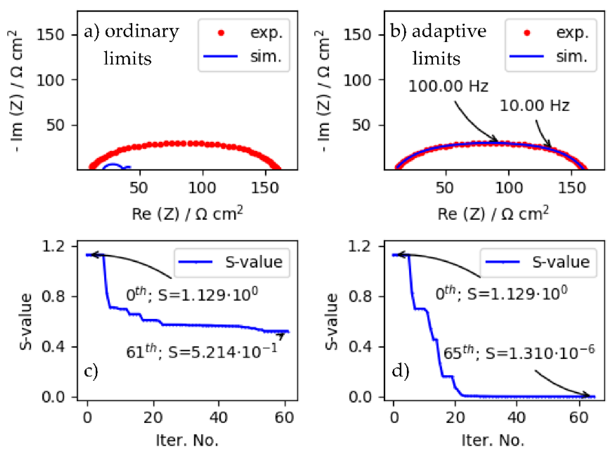
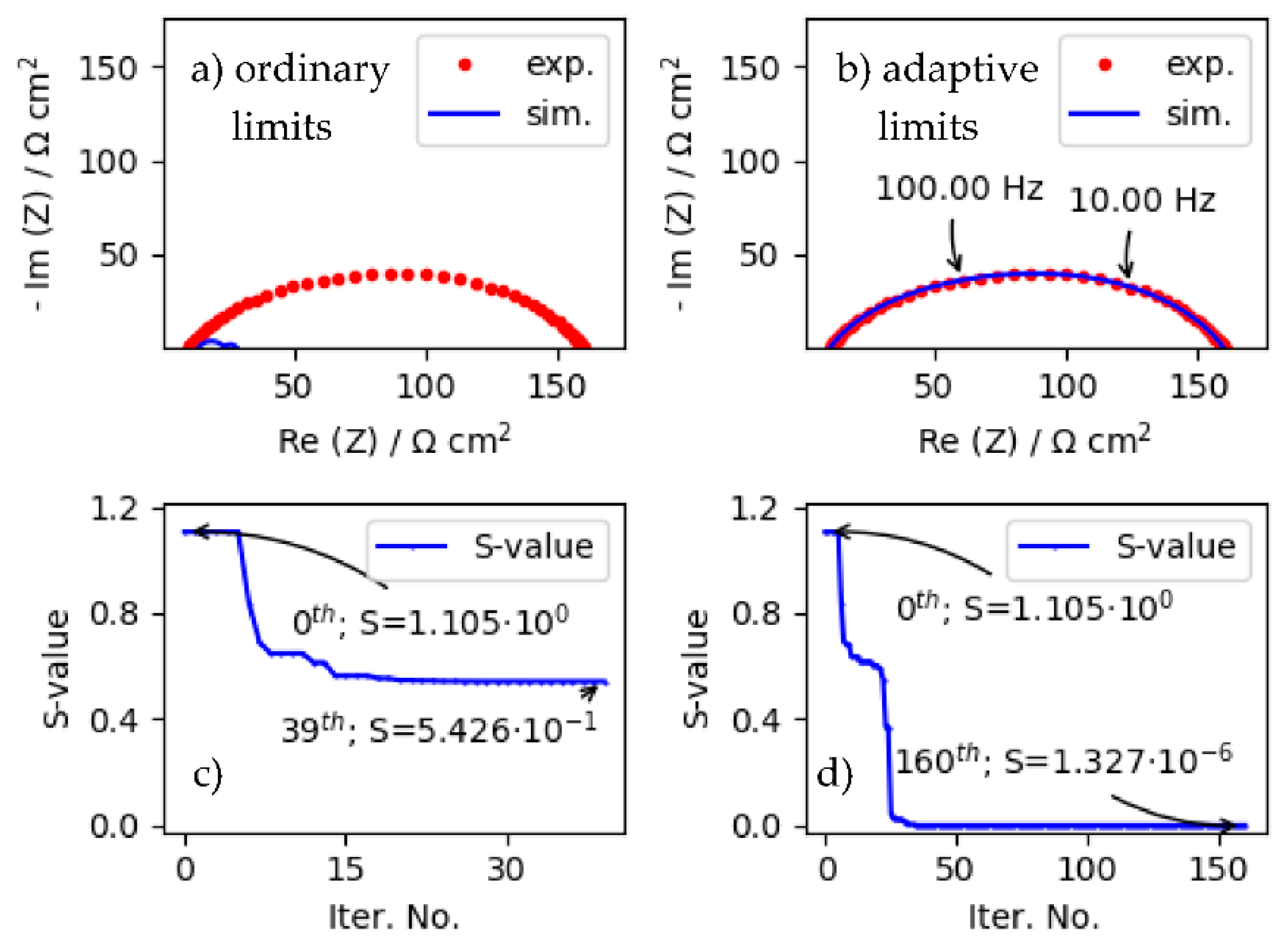
4.2. Impact of Ordinary and Automatic Update (i.e., Adaptive) Limit Strategies on LMA Convergence Properties When Fitting ZARC Data by Using Poor Starting Parameters

In the previous section we demonstrated that the adaptive strategy shows superior convergence properties in the final stages of the fit. In this section, we investigated how the adaptive strategy affects the LMA performance during the early stages, i.e., when faced with a poor starting parameter guess (see Table 3). The aforementioned approach was chosen since it is not always entirely clear how to choose the starting EEC parameter values that correspond to the electrochemical process(es) under study.

According to Figure 3a, the adaptive limit strategy ensured an accurate data match between the ZARC and simulated data. Conversely, the standard limit strategy failed to produce a precise data match, as the limit gap was large and non-adaptive (Figure 3a). Additionally, the adaptive limit strategy yielded the same final parameters values by using both poor and good starting parameters guesses (Table 4). These results clearly indicate that the adaptive limit strategy is more advanced; and consequently, further testing is justified.

According to the S-value curve in Figure 3c, the ordinary limit strategy was stuck in the 61th iteration at a high S-value (5.214 × 10⁻¹). In the equal fitting conditions, the adaptive limit strategy reached a significantly lower S-value (1.310 × 10⁻⁶) after 65 iterations (Figure 3d). The considerably better convergence properties can be explained by the automatic update of the limit gap (Algorithm 3). Finally, the slow reduction in the S-value in the final stage of the fits can be observed in both Figure 3c,d; and thus, it is not governed by the adaptive strategy.

4.3. Impact of Ordinary and Automatic Update (i.e., Adaptive) Limit Strategies on LMA Convergence Properties When Fitting More Corrupted ZARC Data by Using Poor Starting Parameters

The presence of the noise in the ZARC data perturbed the local landscape of the CNLS problem (2). The term local landscape is frequently used when commenting on the local landscape of mathematical functions (e.g., CNLS problem [15]). Moreover, in EIS, τ values of electrochemical processes under the study are of special interest. Therefore, LMA should be able to converge through a corrupted landscape that is characterized by more closely distributed τ values. Herein, we have additionally corrupted the ZARC data (Figure 4), by using more closely distributed (0.01, 0.005 and 0.001 s) τ values (see Table 2).

Figure 4a,c clearly show that the more corrupted local landscape of the CNLS problem was an unsolvable problem when using the ordinary limit strategy. On the other hand, the application of the adaptive limit strategy (Figure 4b,d) resulted in a successful fit after 160 iterations (S = 1.327 × 10⁻⁶). According to

Table 5. Final EEC parameter values obtained by using EEC_{R(QR)(QR)(QR)} and the automatic update limit strategy. The values are obtained by fitting the ZARC data (Figure 4).

EEC Parameters
	k	1	2	3
Rs (Ω cm2)	9.99	-	-	-
Y0,k (S sn cm−2)	-	9.995 × 10−3	3.520 × 10−4	1.500 × 10−4
n	-	0.677	0.714	0.694
R (Ω cm2)	-	7.959	83.441	58.549
aτk (s)		2.386 × 10−2	7.184 × 10−3	1.096 × 10−3

^a estimated τ values $\left({\left(R_k{Y}_{0,k}\right)}^{\frac{1}{n_k}}\right)$.

, the computed τ values (2.386 × 10⁻², 7.184 × 10⁻³, and 1.096 × 10⁻³ s) correspond well to the ones (0.01, 0.05, and 0.001) used to prepare the corrupted ZARC data (Table 2). This test confirms that the adaptive limit strategy is especially suitable for describing electrochemical processes with closely distributed τ characteristics.

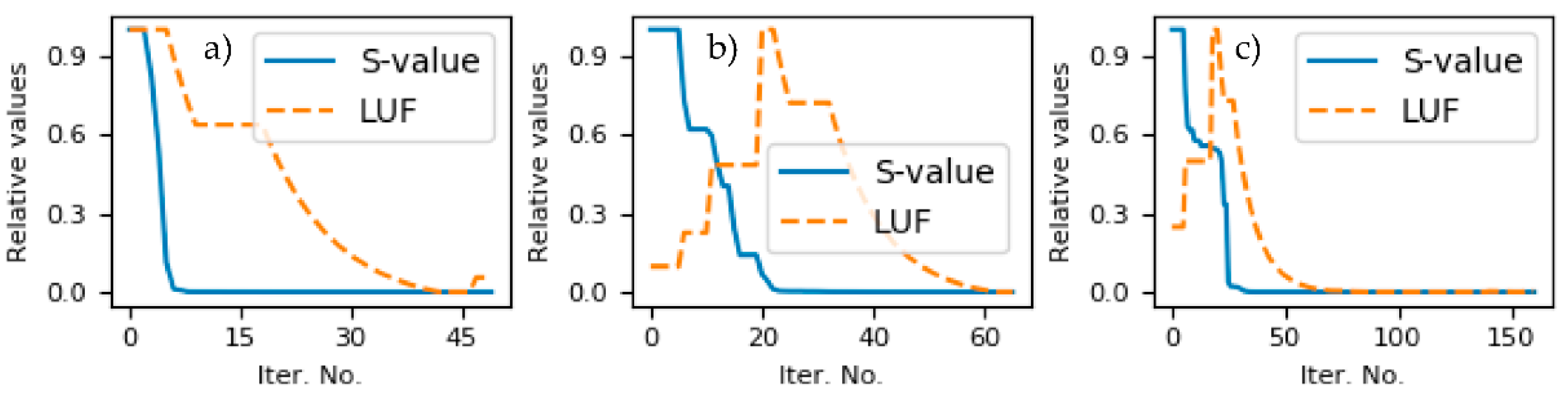
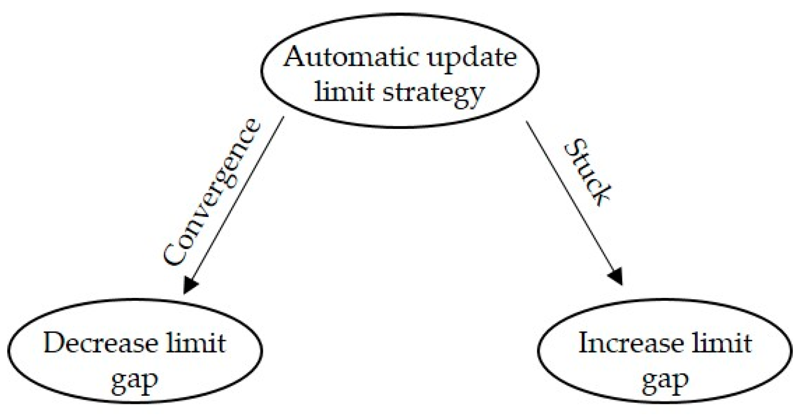
4.4. Automatic Update of LUF Value during LMA Iteration

As S-values and LUF values have a rather different range, they were preprocessed to fit in the [0, 1] interval. This approach will facilitate analyses of the adaptive limit strategy in this Section. Figure 5a,c present S-values and LUF data obtained from fitting attempts given in Figure 2c, Figure 3b and Figure 4b. Thus, several observations can be briefly given. First, at the beginning of fits, S-values (Figure 5) are high for all fitting attempts, but they decrease towards the end of the fit. Second, LUF values are also lower in the final stage of the fit, which additionally ensures the convergence. Third, an increase in LUF values occurs only after LMA becomes stuck in several iterations. To be precise, when the fit becomes stuck, an increase in the LUF values ensures LMA convergence as EEC parameter values can now take more different values from the larger limit gap.

To summarize, Figure 5 clearly shows that the adaptive limit strategy acts oppositely to the trust-region methods, i.e., it decreases the limit gap in the conditions when LMA converges, and it increases LUF values when LMA gets stuck.

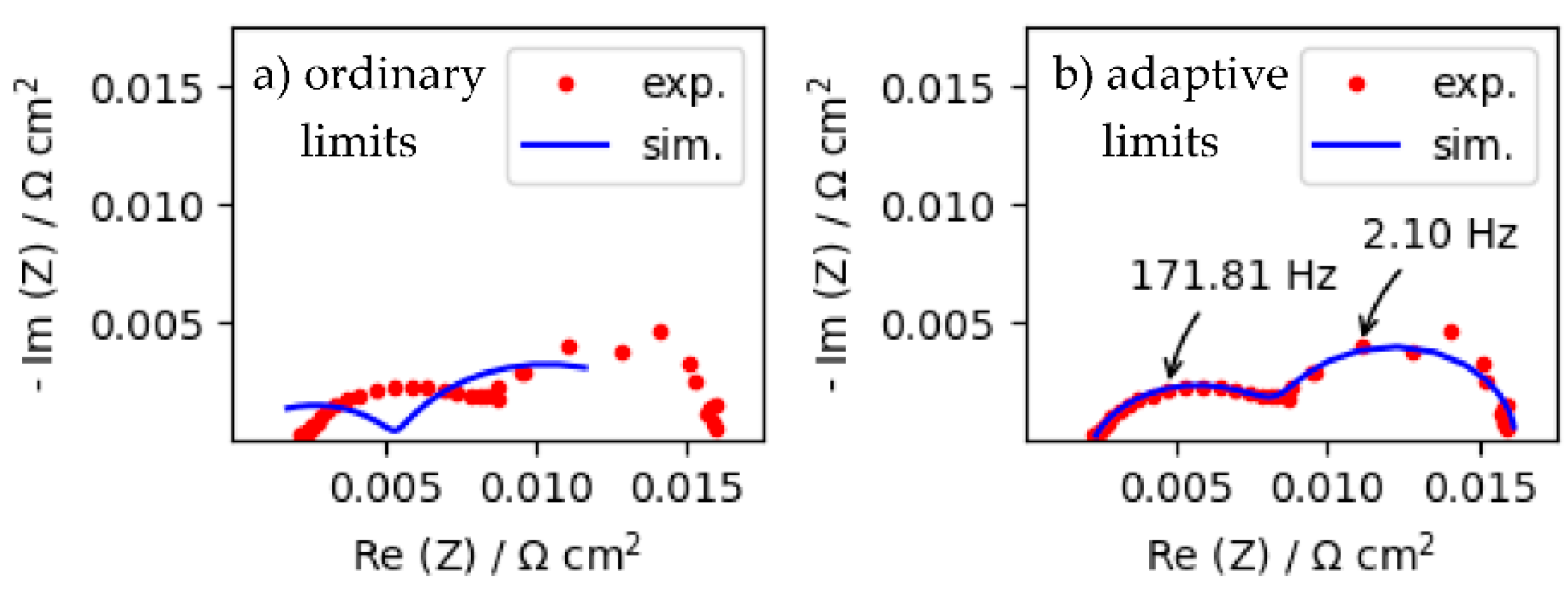
4.5. Experimental SOFC Impedance Data

Impedance response of the applied SOFC is presented in Figure 6. The impedance response in the high frequency region (around 171.81 Hz) is characterized by a depressed semi-circle and with a rather low portion of noise. On the other hand, the semi-circle in the low frequency region (around 2.10 Hz) has a higher portion of noise, which is a consequence of the operating environment. Due to the presence of the noise, it is not clear whether or not this semi-circle is depressed.

Furthermore, there might be several individual processes with similar time-constants in Figure 6; and hence, one can get a false impression that there are only two of them. Nevertheless, to test the adaptive limit strategy, we applied EEC_R(QR)(QR) with two (k = 2; see (12)) serial QR circuits. A poor starting EEC parameters guess was used to test the worst possible fitting scenario (see

Table 6. Final and poor starting (in parentheses) EEC parameter values obtained by using EEC_R(QR)(QR) and the automatic update limit strategy. EEC_R(QR)(QR) was used only for experimental solid oxide fuel cells data fitting. The values are obtained by fitting the experimental data given in Figure 6.

EEC Parameters
	k
		1	2
Rs (Ω cm2)	2.29 × 10−3(1.10)	-	-
Y0,k (S sn cm−2)	-	1.038 (0.01)	14.445 (5.00)
n	-	0.767 (0.63)	0.999 (0.73)
R (Ω cm2)	-	6.427 × 10−3 (0.50)	7.484 × 10−3 (2.50)
aτκ (s)		1.459 × 10−3	1.078 × 10−1

^a estimated τ values $\left({\left(R_k{Y}_{0,k}\right)}^{\frac{1}{n_k}}\right)$.

). In this scenario, when using the ordinary limit strategy, LMA failed to yield a good data match (Figure 6a). On the other hand, the application of the adaptive limit strategy resulted in a good fit (Figure 6b).

Next, τ values in Table 6 display EEC values of two distinguished electrochemical processes characterized by different time constants (1.459 × 10⁻³ and 1.078 × 10⁻¹ s). The first depressed semi-circle in the high frequency region is defined by a low n = 0.767 value, which implies that several electrochemical processes (with similar τ ) might occur simultaneously. The second semi-circle in the low frequency region yielded n = 0.999 value, which suggests the presence of only one process.

Overall, the exercise in this section clearly demonstrated firm evidence that the application of the automatic update limit strategy suppressed the impact of a poor parameter choice. A fair data correlation in Figure 6b unambiguously indicates that the automatic update limit strategy can be used to study the SOFC impedance data.

5. Conclusions

In this work, a new automatic update limit strategy that greatly improves the LMA performances was both demonstrated and evaluated. The new automatic strategy boosted the algorithm to be less reliant on the starting parameter guess.

The new strategy was put to the test by solving several complex nonlinear least-square (CNLS) problems. It was shown that the new strategy can be used to characterize numerous electrochemical processes. The findings in this work clearly demonstrate that the LMA convergence properties are superior when the new automatic update limit strategy is applied.

Herein, the ability of the automatic update limit strategy to finely tune a limit update factor (LUF) value during convergence was tested by solving the CNLS problem characterized by a more corrupted local landscape. The aforementioned exercise pointed out that the new strategy can automatically adjust LUF values during the iteration process.

Finally, the automatic update limit strategy was used to define electrochemical processes that take place in the solid oxide fuel cells of industrial size. We detected two major electrochemical processes that are possibly formed from several processes with similar time constants. Moreover, the high frequency region was characterized by n = 0.767, which confirms that several processes might take place in parallel.

References

1. Subotić, V.; Baldinelli, A.; Barelli, L.; Scharler, R.; Pongratz, G.; Hochenauer, C.; Anca-Couce, A. Applicability of the SOFC technology for coupling with biomass-gasifier systems: Short- and long-term experimental study on SOFC performance and degradation behaviour. Appl. Energy 2019, 256, 113904. [Google Scholar] [CrossRef]
2. Kobayashi, K.; Suzuki, T.S. Development of Impedance Analysis Software Implementing a Support Function to Find Good Initial Guess Using an Interactive Graphical User Interface. Electrochemistry 2019, 88, 39–44. [Google Scholar] [CrossRef] [Green Version]
3. Wan, T.H.; Saccoccio, M.; Chen, C.; Ciucci, F. Influence of the Discretization Methods on the Distribution of Relaxation Times Deconvolution: Implementing Radial Basis Functions with DRTtools. Electrochim. Acta 2015, 184, 483–499. [Google Scholar] [CrossRef]
4. Barsoukov, E.; Macdonald, J.R. Impedance Spectroscopy: Theory, Experiment, and Applications; Wiley: Hoboken, NJ, USA, 2005. [Google Scholar]
5. Zic, M.; Pereverzyev, S., Jr.; Subotić, V.; Pereverzyev, S. Adaptive multi-parameter regularization approach to construct the distribution function of relaxation times. GEM Int. J. Geomathematics 2020, 11, 1–23. [Google Scholar] [CrossRef] [Green Version]
6. Song, J.; Bazant, M.Z. Electrochemical Impedance Imaging via the Distribution of Diffusion Times. Phys. Rev. Lett. 2018, 120, 116001. [Google Scholar] [CrossRef] [Green Version]
7. Pereverzyev, S.V.V.; Solodky, S.G.; Vasylyk, V.B.; Žic, M. Regularized Collocation in Distribution of Diffusion Times Applied to Electrochemical Impedance Spectroscopy. Comput. Methods Appl. Math. 2020, 20, 517–530. [Google Scholar] [CrossRef]
8. Zic, M. An alternative approach to solve complex nonlinear least-squares problems. J. Electroanal. Chem. 2016, 760, 85–96. [Google Scholar] [CrossRef]
9. Kelley, C.T. Iterative Methods for Optimization; SIAM: Philadelphia, PA, USA, 1999. [Google Scholar]
10. Wolberg, J. Data Analysis Using the Method of Least Squares: Extracting the Most Information from Experiments; Springer Science & Business Media: Berlin/Heidelberg, Germany, 2006. [Google Scholar]
11. Nocedal, J.; Wright, S.J. Numerical Optimization; Springer: New York, NY, USA, 1999. [Google Scholar]
12. Levenberg, K. A method for the solution of certain non-linear problems in least squares. Q. Appl. Math. 1944, 2, 164–168. [Google Scholar] [CrossRef] [Green Version]
13. Marquardt, D.W. An Algorithm for Least-Squares Estimation of Nonlinear Parameters. J. Soc. Ind. Appl. Math. 1963, 11, 431–441. [Google Scholar] [CrossRef]
14. Moré, J.J. The Levenberg-Marquardt algorithm: Implementation and theory. In Numerical Analysis; Watson, G.A., Ed.; Springer: Berlin/Heidelberg, Germany, 1978; pp. 105–116. [Google Scholar]
15. Zic, M.; Pereverzyev, S.V.V. Optimizing noisy CNLS problems by using Nelder-Mead algorithm: A new method to compute simplex step efficiency. J. Electroanal. Chem. 2019, 851, 113439. [Google Scholar] [CrossRef]
16. Dellis, J.-L.; Carpentier, J.-L. Nelder and Mead algorithm in impedance spectra fitting. Solid State Ionics 1993, 62, 119–123. [Google Scholar] [CrossRef]
17. Nelder, J.A.; Mead, R. A Simplex Method for Function Minimization. Comput. J. 1965, 7, 308–313. [Google Scholar] [CrossRef]
18. Fajfar, I.; Bűrmen, Á.; Puhan, J. The Nelder–Mead simplex algorithm with perturbed centroid for high-dimensional function optimization. Optim. Lett. 2019, 13, 1011–1025. [Google Scholar] [CrossRef]
19. Fajfar, I.; Puhan, J.; Árpád, B. Evolving a Nelder–Mead Algorithm for Optimization with Genetic Programming. Evol. Comput. 2017, 25, 351–373. [Google Scholar] [CrossRef] [PubMed]
20. Žic, M. Solving CNLS problems by using Levenberg-Marquardt algorithm: A new approach to avoid off-limits values during a fit. J. Electroanal. Chem. 2017, 799, 242–248. [Google Scholar] [CrossRef]
21. Žic, M.; Subotić, V.; Pereverzyev, S.; Fajfar, I. Solving CNLS problems using Levenberg-Marquardt algorithm: A new fitting strategy combining limits and a symbolic Jacobian matrix. J. Electroanal. Chem. 2020, 866, 114171. [Google Scholar] [CrossRef]
22. Madsen, K.; Nielsen, H.B. Introduction to Optimization and Data Fitting; Technical University of Denmark: Lyngby, Denmark, 2008. [Google Scholar]
23. Nielsen, H.B.; Madsen, K.; Tingleff, O. Methods for Non-Linear Least Squares Problems, 2nd ed.; Informatics and Mathematical Modelling, Technical University of Denmark (DTU): Lyngby, Denmark, 2004. [Google Scholar]
24. Nielsen, H.B. Damping Parameter in Marquardt’s Method; Techcinal Report IMM-REP-1999-05; Technical University of Denmark: Lyngby, Denmark, 1999. [Google Scholar]
25. James, F.; Winkler, M. Minuit User’s Guide; CERN: Geneva, Switzerland, 2004; Available online: https://inspirehep.net/files/c92c2ba4dac7c0a665cce687fb19b29c (accessed on 6 December 2020).
26. James, F.; Roos, M. Minuit-A system for function minimization and analysis of the parameter errors and correlations. Comput. Phys. Commun. 1975, 10, 343–367. [Google Scholar] [CrossRef]
27. Sheppard, R.J.; Jordan, B.P.; Grant, E.H. Least squares analysis of complex data with applications to permittivity measurements. J. Phys. D Appl. Phys. 1970, 3, 1759–1764. [Google Scholar] [CrossRef]
28. Zoltowski, P. The error function for fitting of models to immittance data. J. Electroanal. Chem. Interfacial Electrochem. 1984, 178, 11–19. [Google Scholar] [CrossRef]
29. Van Der Walt, S.; Colbert, S.C.; Varoquaux, G. The NumPy Array: A Structure for Efficient Numerical Computation. Comput. Sci. Eng. 2011, 13, 22–30. [Google Scholar] [CrossRef] [Green Version]
30. Hunter, J.D. Matplotlib: A 2D Graphics Environment. Comput. Sci. Eng. 2007, 9, 90–95. [Google Scholar] [CrossRef]
Scheme 1. Impact of the automatic update limit strategy on the limit gap during the Levenberg–Marquardt algorithm (LMA) fit.
Processes 09 00108 sch001
Figure 1. EECR(QR)(RQ)(RQ) model used to fit ZARC data. The model is comprised by using three serial QR circuits. Symbol reference: R—resistor (Ω cm2) and Q—Constant Phase Element (S sn cm−2).
Processes 09 00108 g001
Figure 2. The impedance spectra of the ZARC data (subplots ac) and the corresponding S-value data (subplots df). EECR(QR)(QR)(QR) (Figure 1) was used in the fitting attempts.
Processes 09 00108 g002
Figure 3. The impedance spectra of the ZARC data (subplots a,b) and the corresponding S-value data (subplots c,d). EECR(QR)(QR)(QR) (Figure 1) was used in the fitting attempts.
Processes 09 00108 g003
Figure 4. The impedance spectra of the corrupted ZARC data (subplots a,b) and the corresponding S-value data (subplots c,d). EECR(QR)(QR)(QR) (Figure 1) was used in the fitting attempts.
Processes 09 00108 g004
Figure 5. S-value and limits update factor (LUF) data obtained while using the automatic update limit strategy in (a) Figure 2, (b) Figure 3, and (c) Figure 4. EECR(QR)(QR)(QR) (Figure 1) was used in the fitting attempts.
Processes 09 00108 g005
Figure 6. The impedance spectra of the experimental solid oxide fuel cells data (subplots a,b). EECR(QR)(QR) was used in the fitting attempts. Subplot (a) displays a failed fitting attempt, whilst subplot (b) shows a successful fit. Both fits were commenced by using a poor EEC starting guess (Table 6).
Processes 09 00108 g006