1. Introduction
Mixing is one of the most common and important unit operations among industrial processes. The importance is particularly significant in turbulent flows with accompanying chemical reactions, because reaction time scales can be of similar or even lower orders of magnitude than those for mixing. Consequently, the mixing efficiency in the system is a crucial factor in improving the quality of a desired product. Among different reactor types, confined impinging jet reactors (referred to in this work simply as jet reactors) are often used in processes that require high mixing intensities, such as particle production through precipitation [
1,
2,
3]. This type of reactor enables almost instantaneous mixing at the molecular level (order of milliseconds) and limits the risk of product retention (or clogging in the extreme case) [
4,
5,
6]. Jet reactors are commonly used in industry, among others, as the reactors of choice for the production of particles [
1,
2,
7,
8] or simply as premixers [
9].
In this work, large eddy simulation (LES) was used to predict the course of the reactive mixing process. Currently, LES and particularly its hybrid modes (detached eddy simulation, scale-adaptive simulation, stress-blended eddy simulation, etc.) can be regarded as useful and valuable solutions to simulate a number of complex processes. One of the reasons is the possibility of the prediction of desired processes in a wide range of Reynolds and Schmidt numbers. Another reason is the substantial increase in compute node density in recent years that happened despite a slow-down of the so-called Moore’s law (twice the transistor density increase every two years) [
10,
11]. Last but not least, there was a considerable effort by the scientific community over past years to develop numerical methods for unresolved processes and also for numerical meshes [
12]. All of this makes LES a compelling tool in real-life engineering applications.
The main idea behind LES is that the large turbulence scales are resolved directly from the filtered transport equations, whereas for the small, subgrid scales (SGS), simple models are introduced, as it is assumed that these scales are more uniform and isotropic. LES provides more physical results in the case of systems with varying flow regimes, whereas using Reynolds-averaged Navier–Stokes (RANS) models in such cases might result in inaccurate predictions [
4,
13,
14,
15,
16,
17]. In jet reactors, similar behavior can be observed, i.e., the laminar and turbulent flow can coexist in different parts of the reactor. With increasing Reynolds number values above 100–125, one can observe the transition from a fully segregated flow regime to the self-sustainable chaotic flow [
18]. This transition is often accompanied by noticeable increase in the mixing speed that can sometimes be misinterpreted as turbulent mixing, which tends to occur at higher Reynolds number values. Hence, the use of RANS models is limited in this case. More information regarding these phenomena can be found in [
4,
15,
16,
18,
19].
Other authors [
6,
7,
20,
21,
22,
23] have made important contributions on the topic of computational fluid dynamics (CFD) modeling of jet reactors. However, their works were focused more on LES modeling of similarly sized reactors, or the included scale-up analysis did not cover LES modeling. Hence, this work has two aims: The first is to better explain and improve our understanding of the reactive mixing process carried out in jet reactors, i.e., the effect of mixing on the final selectivity of the chemical reaction, using two commonly available turbulence models. The second is to validate the proposed modeling approach (the turbulence, concentration variance, and closure models used) as a useful tool in reactor design.
To characterize the mixing process, a set of two competitive, parallel chemical reactions with well-known kinetics was used. The reaction system consisted of the neutralization of sodium hydroxide with hydrochloric acid and the alkaline hydrolysis of ethyl chloroacetate [
24]. The LES results were validated by experimental data and compared with the
k-ε model predictions that served as a good reference point. The interpretation of the CFD predictions enabled basic reactor design guidelines to be drawn up. In this contribution, we present an energetic efficiency analysis, and assessed the prediction capability for the reactive mixing of both turbulence models.
4. Simulation Setup
Hydrodynamics in the mixers were predicted using ANSYS Fluent CFD software. Two turbulence models were employed: the realizable k-ε (RANS) model with the “enhanced wall treatment” option enabled and large eddy simulation coupled with the Smagorinsky–Lilly dynamic stress model. The RANS simulations served as a startup point and benchmark for LES.
The size of numerical grids was differentiated by the outlet pipe diameter. For = 11 mm (I, II), meshes were made of approximately 800,000 hexahedral cells, whereas for = 2 mm (III) there were approximately 300,000 hexahedral cells. The meshes were the densest in the mixing chamber region and the near-wall cell sizes were set accordingly to satisfy the y+~1 condition. The mesh independence was checked at the highest tested Reynolds numbers using two quantities: average wall shear stress value at the walls and average turbulence energy dissipation rate value in the system. The results of both of these quantities were constant (less than 3% difference), even with using denser meshes than those described.
To minimize the numerical diffusion, a bounded central differencing scheme was applied to all turbulence quantities, whereas a second-order discretization scheme was used for the pressure and scalars. The value of 10
−6 or smaller for normalized residuals was considered as a fulfilled convergence condition. The averaged values predicted by large eddy simulations were obtained for a time interval equal to 10 residence times,
. The residence time was defined as
=
/
, where
V is the reactor volume and
is the total flow rate in the system. The time step value was set individually to meet the
≤
/
condition [
28], where
is the time step value,
is the numerical cell size (cube root of its volume), and
U is the local velocity magnitude in the cell.
The transport equation for the filtered mean mixture fraction,
, in LES is expressed as
where ¯ indicates a filtered value,
is the molecular diffusivity, and
is the subgrid diffusivity. In this work,
was determined using the following formula [
29]:
where
is the eddy viscosity, and
is the subgrid Schmidt number. In LES simulations,
was calculated using an algebraic model—the Smagorinsky model with local adaptation of the Smagorinsky constant [
30,
31].
To predict the course of parallel chemical reactions, the probability density function (PDF) closure method using conditional moments and the probability density function (PDF), approximated in this case by the Beta function, was used [
13]:
where
The PDF describes the subgrid-scale inhomogeneity based on the subgrid scale concentration variance value,
. However, the subgrid concentration variance cannot be calculated directly from the conservation equation of the filtered mixture fraction (Equation (5)), and another balance equation is necessary. One possible solution was proposed by Cook and Riley [
32]. This was based on the assumption that the small scale phenomena can be estimated from the slightly larger scales using the filtering operation. The proposed model [
32] was based on a constant coefficient, the value of which was determined by Cook [
33] for the mixing of gases, ranging from 0.54 to 1.75. In the case of liquids (high Schmidt numbers), the coefficient value increases, reaching the asymptotic value of 5 [
34]. However, such model definition with a constant coefficient limits the description of the local flow characteristics, i.e., the local changes of the Reynolds and Schmidt number values. To overcome this issue, one can use the scale similarity model supplemented with the dynamic model coefficient [
17]:
where
indicates a test-filter (
),
is the Kolmogorov scale,
is the Batchelor number, and
is the turbulence kinetic energy dissipation rate. The main advantage of the model is that it does not require using any a priori defined coefficients and can be used for fluids with variable Schmidt numbers. The details regarding the model can be found in one of the previous works of the authors [
15,
17]. To predict the concentration variance distribution in the systems using the RANS model, the
k-ε model was additionally supplemented with the turbulent mixer model [
24,
35].
A set of filtered differential balance equations for any reacting species is then solved:
The first reaction, given by Equation (2) is assumed to be instantaneous and the rate of the second reaction is expressed as
where
The physical meaning of Equation (13) is the linear interpolation between an infinitely slow and instantaneous reaction.
The closure can be applied to both LES and RANS models, where in RANS it is used for the whole spectrum of turbulent concentration fluctuations, and in LES at the subgrid level.
5. Results and Discussion
In this work, the following numerical approach was taken to predict the course of parallel chemical reactions. In the first stage, we studied the hydrodynamics in the systems. This stage consisted of predictions of velocity, tracer concentration, and tracer concentration variance profiles in the systems. In the next phase, the closure model for the chemical reaction was applied. Both of these phases were conducted using the LES and
k-ε models. Such an approach enabled easy verification of each modeling phase and worked well for simulations of reactive mixing both in general and in the specific case of jet reactors [
15,
36].
In the case of velocity and tracer concentration distribution in jet reactors, LES generally produced more accurate results, as was shown in our previous works [
15,
16]. We demonstrated that, at lower jet Reynolds numbers (
Rejet), the RANS results can differ significantly from the experiments, whereas, at higher jet Reynolds numbers, the discrepancy between both the LES results and experiments decreased. The results indicated that the
k-ε model failed to properly predict the flow behavior, i.e., a collision of inlet streams and resulting fluid motion around the outlet pipe and impingement zone [
16]. This follows from the theory of turbulence and is related to the Reynolds-averaged approach. In this approach, the variation of time-averaged quantities occurs at relatively large scales and does not necessary resolve all small-scale phenomena, both temporal and spatial [
37].
Although the differences between the RANS and experimental results can be large, this may not necessarily make the RANS models unusable to qualitatively assess jet reactor performance. That is because the regions where the largest discrepancies were observed were small compared to the reactor volume, and the residence time in these regions is very short (order of milliseconds). The residence time decreases even further with the increasing Reynolds number. This applies especially to processes that are slower than mixing.
In the case of parallel chemical reactions that are fast compared to mixing, one can expect the discrepancies to increase with decreasing Reynolds numbers. This can be observed in
Figure 4,
Figure 5,
Figure 6 and
Figure 7, which show a comparison of the final selectivity predictions of both turbulence models with experimental data. The experiments and calculations were performed for
= 300 ÷ 4000 for the reactors with
= 4.6 or 7 mm (V-mixer I, V-mixer II, SP-mixer I, L-mixer I and T-mixer I, and T-mixer II) and
= 50 ÷ 1000 for the reactors with
= 1.45 mm (T-mixer III and V-mixer III). The results for the T-mixer I and T-mixer II were presented in the authors’ previous work [
15], and one can observe that they are similar to those for other reactors presented in this work.
is defined as:
where
is the mean velocity in the jet (inlet pipe),
= 997 kg m
−3 is the density, and
= 0.891 × 10
−3 Pa s is the dynamic viscosity of the inlet solutions at 298 K.
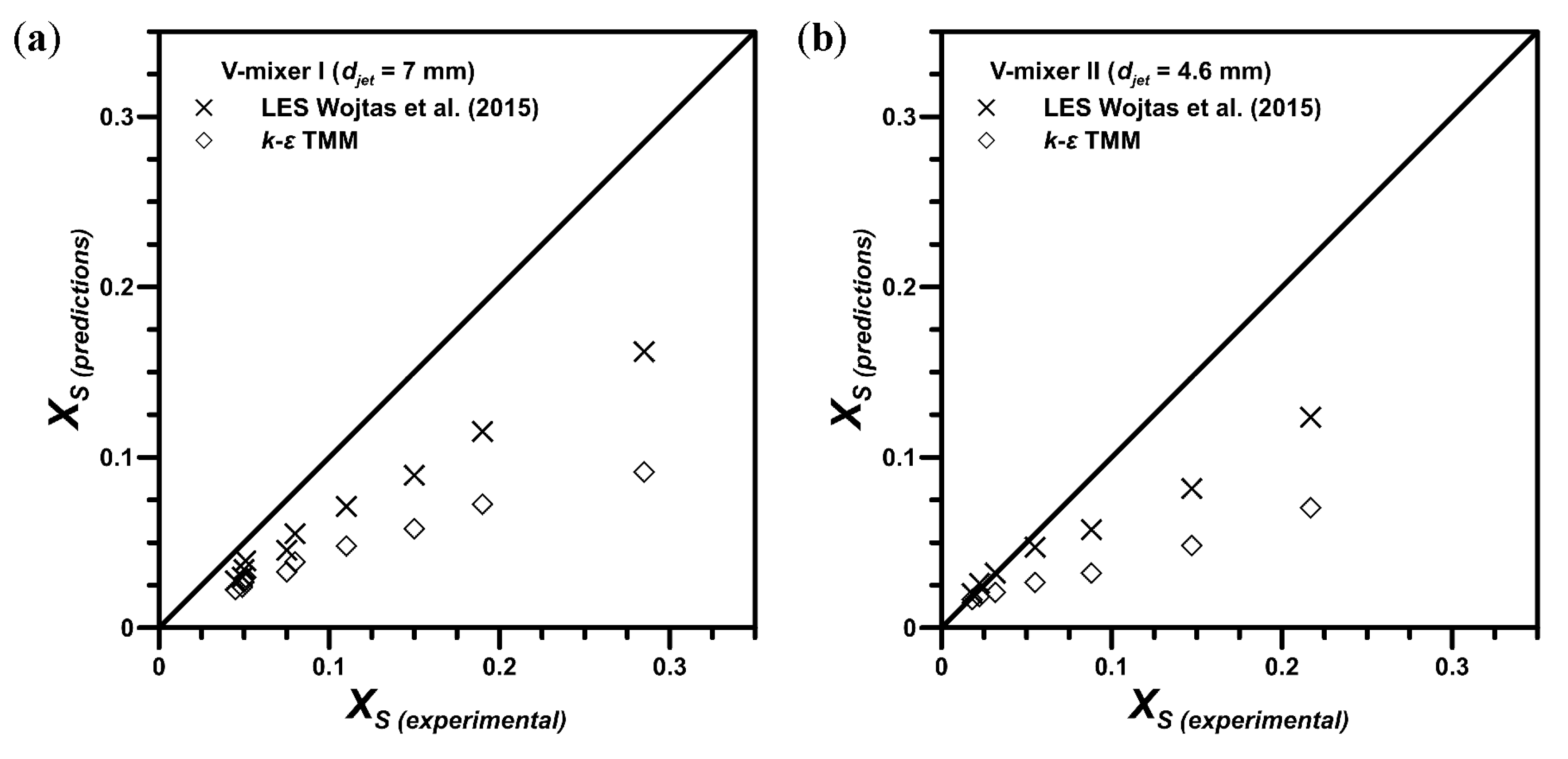
The effect of
on the final selectivity of the slower reaction for the V-mixer I (
= 7 mm) and V-mixer II (
= 4.6 mm) is shown in
Figure 4. The LES model agreed better with the experiments for the whole tested range of
, i.e., regardless of turbulence intensity that is characterized here by low and high
values for high and low intensity, respectively. The
k-ε model, on the other hand, gave acceptable results solely at the highest tested jet Reynolds number values, when the turbulence was more intense and the mixing mechanism was dominated by inertial convective effects. This is more clearly visible in
Figure 5, which shows the differences between the LES and RANS predictions presented in a form of parity plot.
However, although advantages of using LES can be seen at both low and high turbulence intensity, the cost of using large eddy simulations is still a real concern for high Reynolds number flows, due to the mesh resolution requirements in a boundary layer [
38,
39]. One can estimate that, for highly turbulent flows (
> 10
5), calculations would be, at best, a million times more costly than for RANS models [
38,
40,
41]. Of course, that makes it rather unrealistic that LES will become a major element of industrial CFD simulations; however, LES can still play a role in the detailed analysis of the elements of such flows. One possible solution for these extreme requirements can be LES hybrid methods, i.e., a combination of RANS in slender, near-wall regions and LES in regions away from walls. In near-wall regions, the turbulence is closer to having mature and repeatable behavior and is more likely to be accurately predicted by simpler models. Overall, pure LES for industrial flows is likely to be limited in the foreseeable future to free-shear flows or simpler geometries, such as jet reactors, preferentially at low to mid Reynolds numbers. Taking this into consideration, the
k-ε model appears to be a reasonable choice for predicting of the course of a chemical reaction in a high Reynolds number regime (
> 3000) or to determine a trend of changes in the process course depending on the process parameters.
The primary reason for the RANS results underestimation lies in an overestimation of the mixing speed and concentration variance values in the reactors, where the largest differences were observed in and near the impingement zone [
15,
16,
17,
36]. These works demonstrated that the differences between the experimental and simulation data for concentration variance were present for both turbulence models. However, the shape of the variance distribution obtained by LES, which is closely related to the mixing area, was well predicted. Conversely, the residence time in this zone decreased with increasing
as was already discussed in this section. Together with the fact that the
k-ε model and closure method were designed to be used for fully turbulent flow simulations, this explains the improving compliance of the RANS results at high
values.
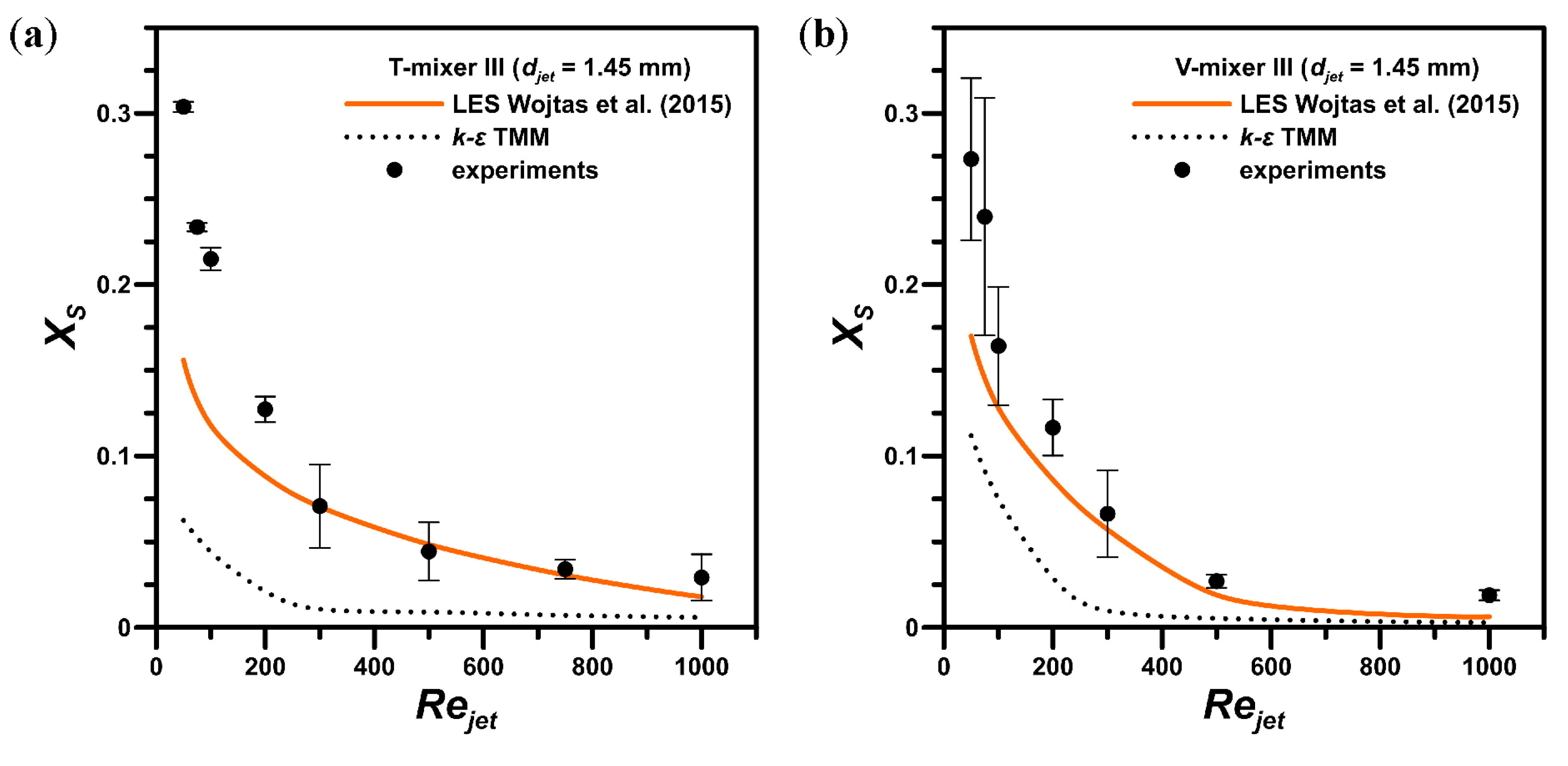
The same situation occurred for the T-mixer III and V-mixer III (
= 1.45 mm), which is shown in
Figure 6. The LES results were more similar to the measurements, and more importantly, the trend of changes of the final selectivity agreed better with the experimental data. At
higher than 500, there was small to no improvement in the mixing quality in the systems. This was a much lower value than in the larger reactors, for which this “critical”
value was around 1500–2000. The position of these points are functional dependent on the chemical concentration (speed of the reaction), hence they are not universal for a specific mixer geometry. We can conclude here that the reactors made in a smaller scale allowed better mixing at much lower flow rates (lower final selectivity values). A physical explanation for this behavior lies in Fick’s law, i.e., the diffusional mixing time is proportional to the square of the characteristic length scale, which decreases as the geometry size becomes smaller. With a decrease in the flow rates, the residence time increases, and so there is more time for the diffusion of species.
A possible reason for the discrepancy between the LES and experimental results at low
values observed for all studied systems lies in the discretization schemes used in the simulations (bounded central differencing for momentum and second-order upwind for scalars). When using implicit filtering in LES as in this work (the filter corresponds to the numerical grid size), the energy content of the smallest resolved scales was underpredicted due to numerical diffusion [
42]. The same underprediction applies to the concentration variance, as the model used [
17] is related to the resolved scalar gradient, which is the largest on these scales. Therefore, one could argue that concentration variance models that employ algebraic relations with respect to resolved scalar or scalar gradient should be used when numerical schemes of higher-order accuracy are applied [
42]. Upwind schemes or bound-preserving limiters are often used in LES as they can mitigate dispersive scalar oscillations; however, both these methods introduce artificial dissipation that can lower the accuracy of predictions [
43].
The solution would be to use more complex methods, but at the time of writing this manuscript, the choice of discretization methods in ANSYS Fluent was limited. The possible options included, among others, second-order upwind, QUICK, third-order MUSCL, and bounded central differencing schemes for the momentum transport equation (with the last one as the recommended setting). As for the scalar transport equation, the choice was limited even further, without the possibility to use central differencing schemes. Given the above, the only way to surmount the problem would be to use different software or even to write custom CFD code supplemented with other numerical schemes, such as the finite-volume WENO scheme [
44], which has been proven to work with minimal dissipation [
43]. However, that was not within scope of this study.
The presented results so far indicate that by slightly changing the reactor geometry, better mixing in the systems could be obtained (lower
values for the V-mixer III). What is more, comparing
Figure 4 and
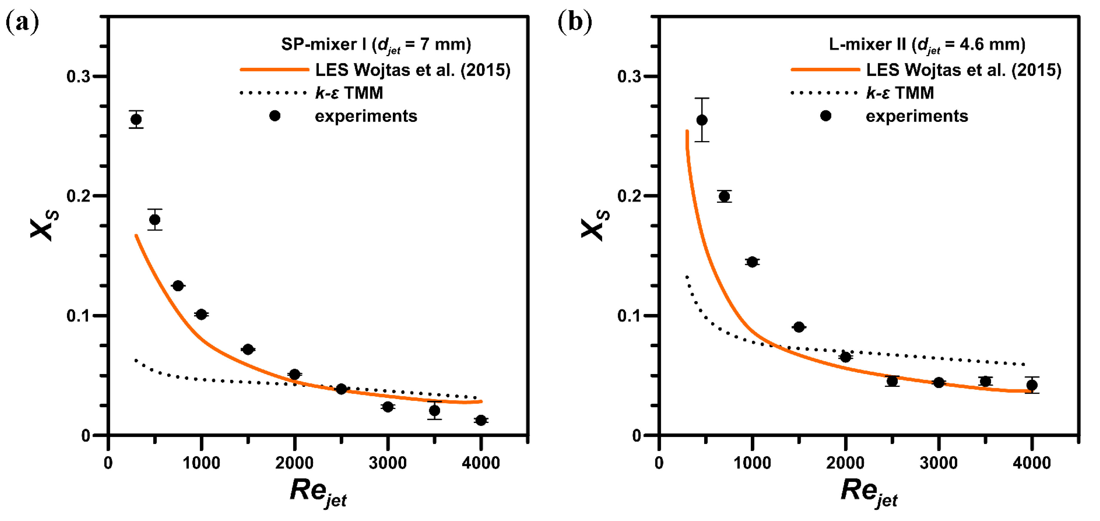
Figure 6, a system scale reduction is one more method of increasing the mixing efficiency in the systems. As the scale reduction and geometry modifications are efficient methods to improve the mixing intensity, we can also consider other types of jet reactors to find a better reactor design. The results obtained for such different designs, i.e., the SP-mixer I (
= 7 mm) (
Figure 3a) and L-mixer II (
= 4.6 mm) (
Figure 3b), are presented in
Figure 7.
By introducing static mixers into the inlet pipes, the SP-mixer I (
= 7 mm) became very similar to the V-mixer II (
= 4.6 mm) in terms of the mixing efficiency, even though it had a larger inlet pipe diameter. As for the L-mixer II (
= 4.6 mm), at low
values, it quickly reached a turnover point, after which no significant improvement in the mixing intensity was observed. The experimental results also indicated that this geometry, in addition to being an interesting construction, offered mediocre mixing conditions, i.e., the final selectivity values were almost identical as in the case of the T-mixer II [
15] and higher than in the V-mixer II (
Figure 4b). The LES results for both reactors agreed well with the experiments at all studied jet Reynolds number values. This again shows the advantage of using large eddy simulations to predict complex chemical processes.
Given the above results, it is difficult to distinguish the most efficient reactor design from all studied jet reactors. Although the smallest mixers allow achieving the lowest values of the final selectivity, their very small dimensions create different problems. One such problem is an even distribution of solutions into the reactor in a continuous operation process, because the small inlet diameters require using syringe pumps. Furthermore, one can expect a much higher pressure drop inside the mixing chamber than in the reactors made in the larger scale. The reactors made in a larger scale also allow high mixing efficiency, but, on the other hand, require high flow rates.
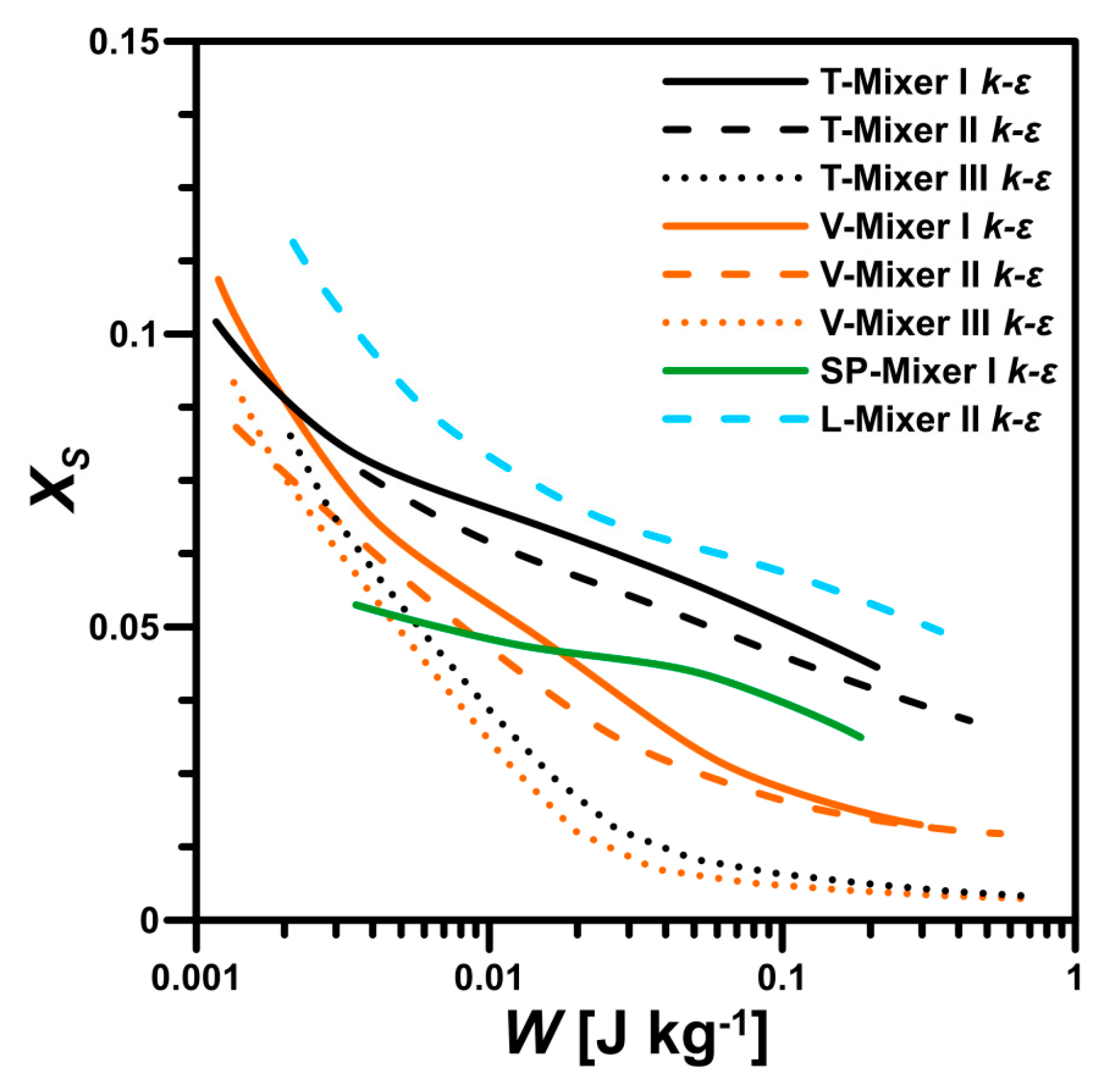
For this reason an energy (economic) analysis becomes helpful. Considering a mixing zone defined as reactor volume in which the chemical reaction occurs, together with the total energy dissipation rate in this zone and total inlet stream, one can calculate the energetic unit cost of obtaining a product as follows:
where
is the mean energy dissipation rate in the reaction zone,
is the residence time in the reaction zone,
is the reaction zone volume, and
is the total flow rate through the reactor. The reaction zone volume was determined based on an area of sodium hydroxide concentration, which was a limiting component in the course of the process.
The results of this analysis are presented in
Figure 8. The results are based on the
k-ε model predictions, as it was shown that, despite the discrepancies, the RANS model correctly predicted the data trends and can be used in a qualitative assessment of the studied reactors. The most important assessment should be made at higher tested jet Reynolds number values, i.e., at the lowest obtained final selectivity values. These values correspond to the right-hand side of
Figure 8, and, as shown in
Figure 4,
Figure 5,
Figure 6 and
Figure 7, are almost identical both for LES and the
k-ε model.
It is clear that with the improved quality of mixing the process cost increases. More importantly, however, certain reactors were more energy-efficient than others. At almost any energy input, the T-mixer III and V-mixer III systems offered the best quality product, characterized here by low values. However, the aforementioned difficulties in the usage of such small geometries remain a concern. As for the larger scale reactors, the vortex T-mixers were the most efficient systems, with a small, but not significant advantage to the V-mixer II. Among the larger scale symmetric T-mixers, introducing static mixers into the system presented certain advantages. It can improve the mixing, as well as reduce the cost of the product.
Concluding the presented results, LES modeling provided better and more agreeable results with the experiments than those obtained using the k-ε model. This was particularly true for low jet Reynolds numbers and illustrates the importance of the effect of large scale inhomogeneities that are neglected by RANS as opposed to LES. Taking this into consideration, LES is a very promising method for obtaining accurate results, especially for processes where the flow changes from laminar to turbulent and vice versa. This is one of many reasons why LES models and the derivatives (hybrid RANS-LES) should be constantly developed, and, in particular, at the subgrid scale, to be successfully used for describing the course of chemical processes.
6. Conclusions
We used competitive, parallel chemical reactions to experimentally characterize the mixing in confined impinging jet reactors. Several systems of different geometry and size were tested. The main aims of the presented work were to validate the modeling procedure used as a useful tool in reactor design and to choose the best reactor in terms of the quality and efficiency of mixing. The methods used in this work, which involved conducting simulations and corresponding experiments (verification step), proved to provide valuable and reliable results.
The presented results showed that LES supplied with the appropriate closure models (for concentration variance and chemical reaction) can be successfully used in the reactor design stage not only for the analysis of various, not described here jet reactors, but also for more complex geometries. The results also enabled us to choose the most favorable of the studied reactor geometries in terms of product quality. The product quality in this case was the highest mixing intensity (lowest final selectivity) and efficiency. In this work, the T-mixer III and V-mixer III (both with equal to 1.45 mm) were found to be superior in this respect. The mixing characteristics, i.e., the increase of mixing quality with the increase of the jet Reynolds number, were apparent for both larger and smaller systems.
The turnover point, at which there was small to no improvement in the final selectivity, occurred at approximately = 2000 for larger reactors ( = 7 mm or 4.6 mm), whereas, for the smallest reactors ( = 1.45 mm), it was at = 500. At this point, the mixing stopped being a dominant rate controlling mechanism in the studied process. Considering these results, i.e., generally lower obtained final selectivity values and the better energetic efficiency in the smallest jet reactors, these systems should be used when the highest mixing intensity is of the highest priority, e.g., in particulate processes.
The results obtained for both the LES and k-ε models supplemented with full closure differed from each other at low Reynolds number values. This is related to the mixing being slower than the chemical reaction and the differences in the hydrodynamic predictions in the mixing chamber for both models. With increasing jet Reynolds number values, the residence time in the impingement zone decreased, making these differences insignificant. The trend of changes was predicted well by both turbulence models, thus, allowing for reactor comparison in terms of the energetic efficiency. Therefore, we conclude that LES supplemented with a PDF closure can be successfully applied to predict the course of the reactive mixing process in jet reactors, while the k-ε model can only be used for qualitative assessment or at high Reynolds numbers (fully developed turbulent flows).


