CFD-DEM Simulation of a Coating Process in a Fluidized Bed Rotor Granulator


Abstract
1. Introduction
2. Model Description
2.1. CFD Modeling
2.2. DEM Modeling
2.3. Contact Force
2.3.1. Capillary Force
2.3.2. Viscous Force
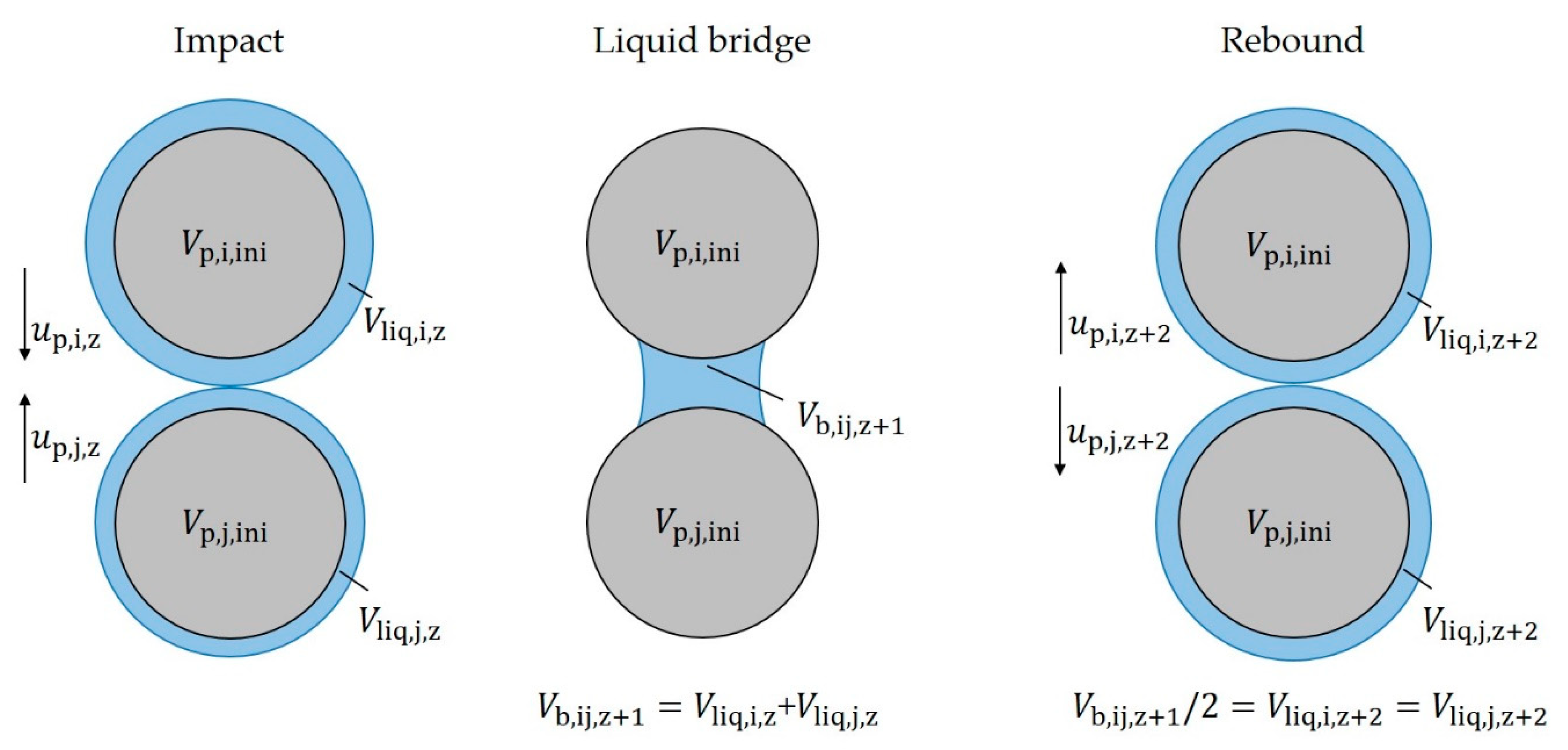
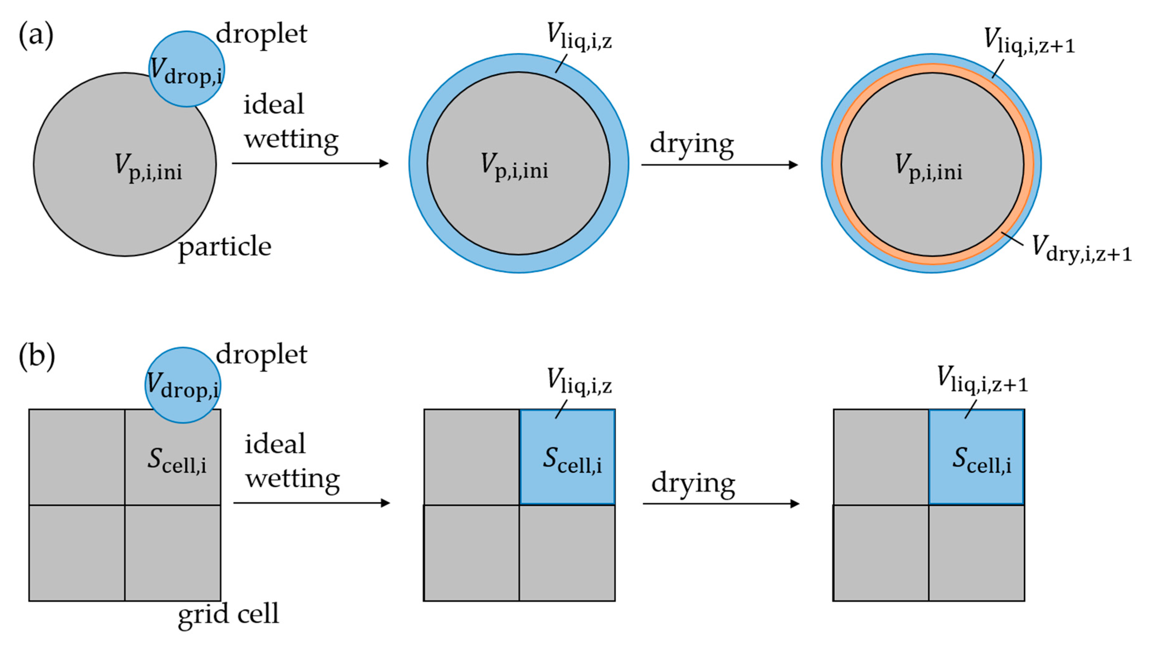
2.4. Coating Model
3. Simulation Setup
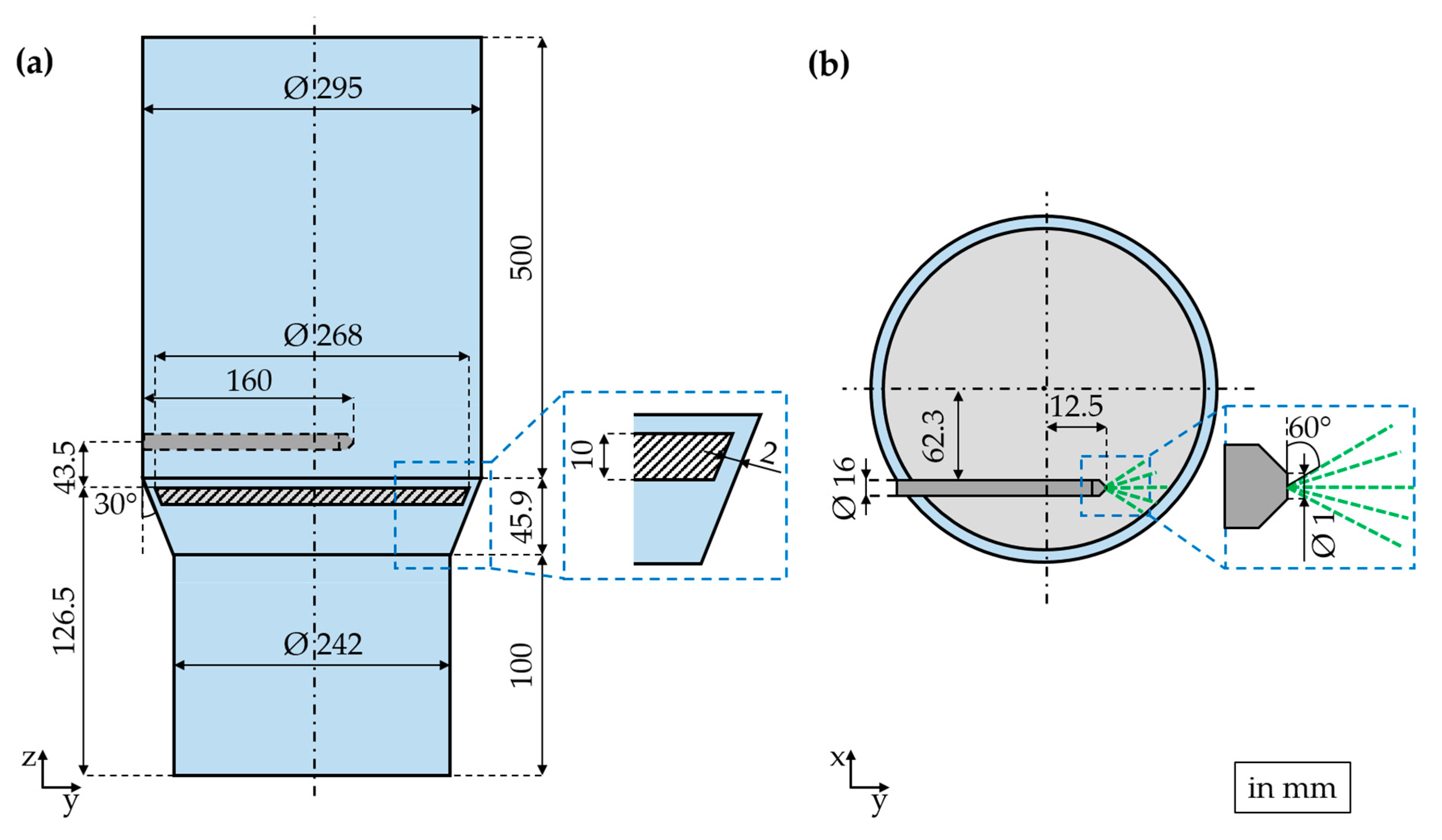
3.1. Geometry of the Rotor Granulator
3.2. Simulation Parameters
4. Results
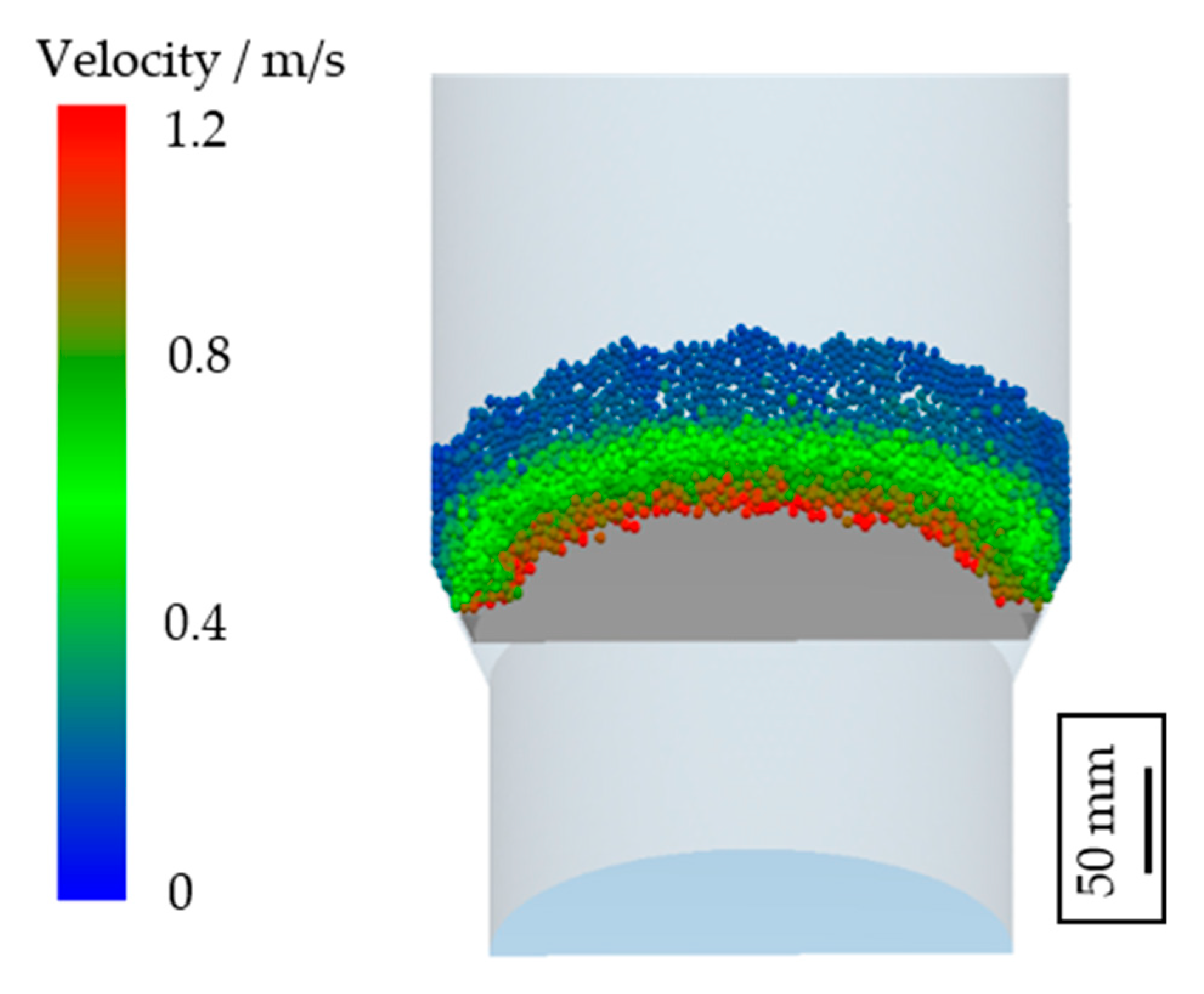
4.1. Influence of Liquid Injection on Particle Dynamics
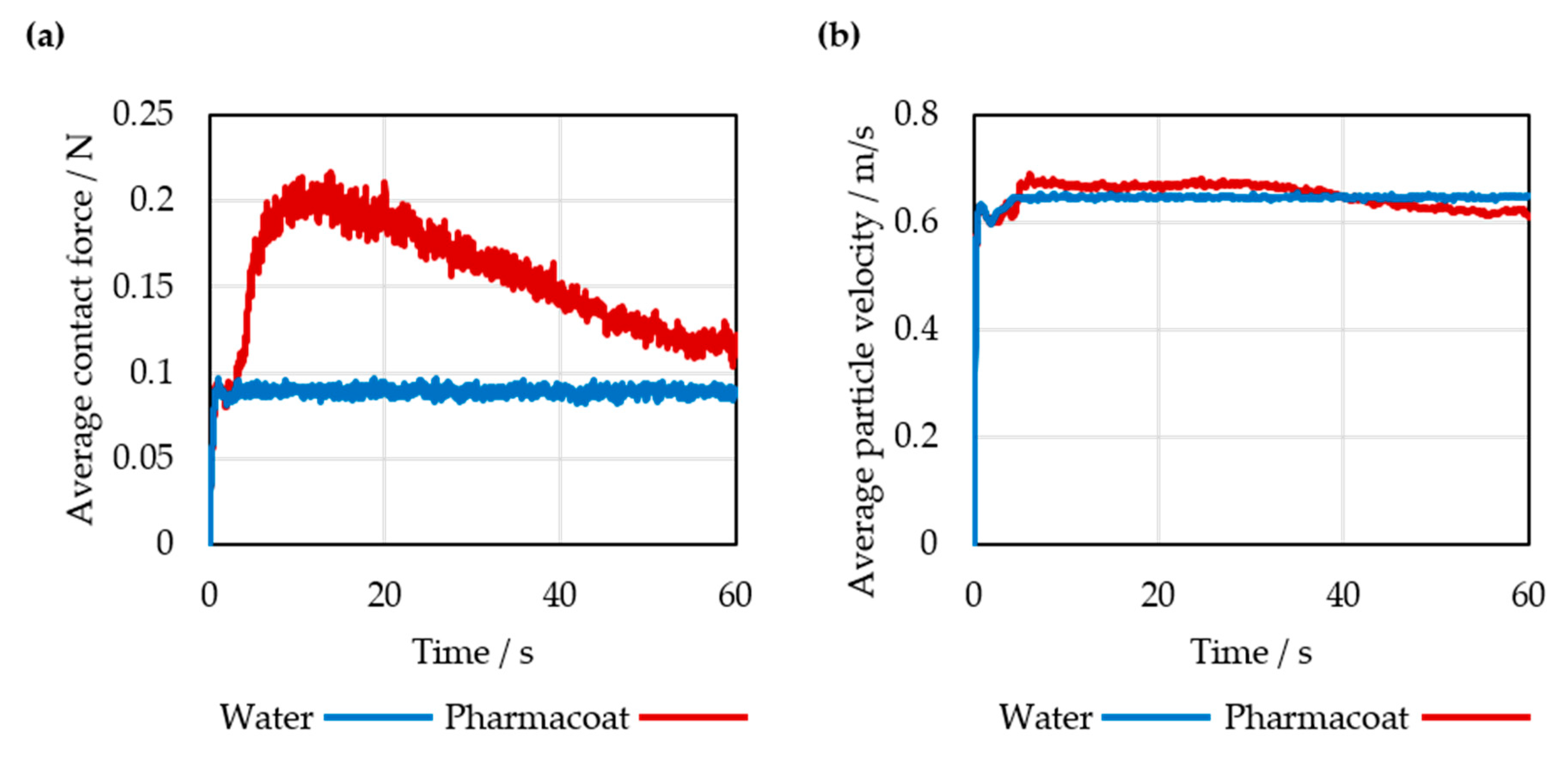
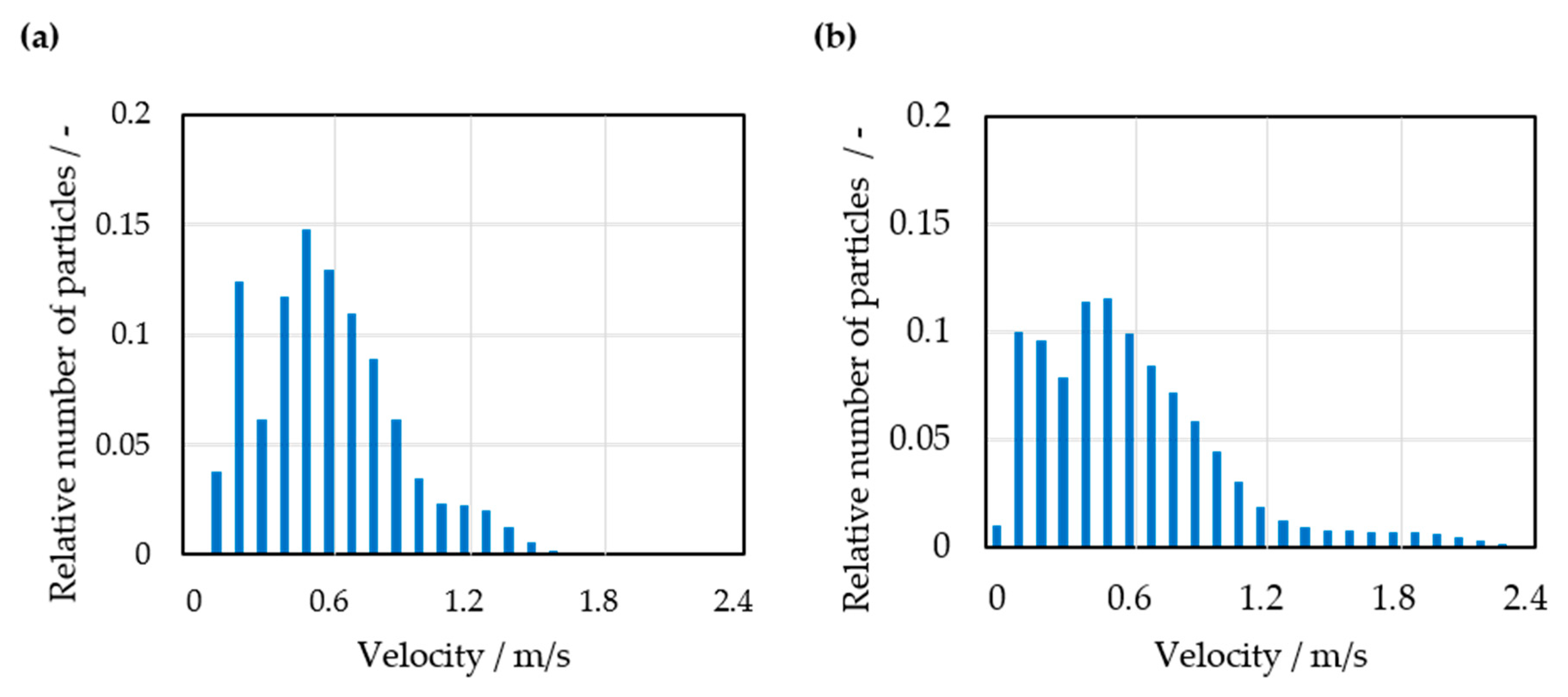
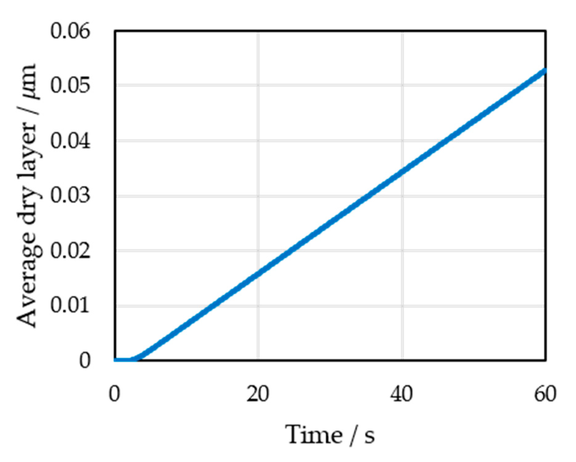
4.2. Influence of the Water Spray Rate and Coating Solution
5. Conclusions
Author Contributions
Funding
Conflicts of Interest
References
- Heinrich, S.; Dosta, M.; Antonyuk, S. Multiscale Analysis of a Coating Process in a Wurster Fluidized Bed Apparatus. Mesoscale Modeling in Chemical Engineering Part I; Elsevier: Amsterdam, The Netherlands, 2015; pp. 83–135. ISBN 9780128012475. [Google Scholar]
- Grohn, P.; Weis, D.; Thommes, M.; Heinrich, S.; Antonyuk, S. Contact Behavior of Microcrystalline Cellulose Pellets Depending on their Water Content. Chem. Eng. Technol. 2020, 43, 887–895. [Google Scholar] [CrossRef]
- Neuwirth, J.; Antonyuk, S.; Heinrich, S.; Jacob, M. CFD-DEM study and direct measurement of the granular flow in a rotor granulator. Chem. Eng. Sci. 2013, 86, 151–163. [Google Scholar] [CrossRef]
- Korakianiti, E.S.; Rekkas, D.M.; Dallas, P.P.; Choulis, N.H. Sequential optimization of a pelletization process in a fluid bed rotor granulator. J. Drug Deliv. Sci. Technol. 2004, 14, 207–214. [Google Scholar] [CrossRef]
- Langner, M.; Kitzmann, I.; Ruppert, A.-L.; Wittich, I.; Wolf, B. In-Line particle size measurement and process influences on rotary fluidized bed agglomeration. Powder Technol. 2020, 364, 673–679. [Google Scholar] [CrossRef]
- Gidaspow, D. Multiphase Flow and Fluidization. Continuum and Kinetic Theory Descriptions; Elsevier Science: San Diego, CA, USA, 1994; ISBN 9780122824708. [Google Scholar]
- Yang, N.; Wang, W.; Ge, W.; Li, J. CFD simulation of concurrent-up gas-solid flow in circulating fluidized beds with structure-dependent drag coefficient. Chem. Eng. J. 2003, 96, 71–80. [Google Scholar] [CrossRef]
- Armstrong, L.M.; Gu, S.; Luo, K.H. Study of wall-to-bed heat transfer in a bubbling fluidised bed using the kinetic theory of granular flow. Int. J. Heat Mass Transf. 2010, 53, 4949–4959. [Google Scholar] [CrossRef]
- Loha, C.; Chattopadhyay, H.; Chatterjee, P.K. Effect of coefficient of restitution in Euler-Euler CFD simulation of fluidized-bed hydrodynamics. Particuology 2014, 15, 170–177. [Google Scholar] [CrossRef]
- Adamczyk, W.P.; Klimanek, A.; Białecki, R.A.; Węcel, G.; Kozołub, P.; Czakiert, T. Comparison of the standard Euler–Euler and hybrid Euler-Lagrange approaches for modeling particle transport in a pilot-scale circulating fluidized bed. Particuology 2014, 15, 129–137. [Google Scholar] [CrossRef]
- Deen, N.G.; van Sint Annaland, M.; Van Der Hoef, M.A.; Kuipers, J.A.M. Review of discrete particle modeling of fluidized beds. Chem. Eng. Sci. 2007, 62, 28–44. [Google Scholar] [CrossRef]
- Salikov, V.; Heinrich, S.; Antonyuk, S.; Sutkar, V.S.; Deen, N.G.; Kuipers, J.A.M. Investigations on the spouting stability in a prismatic spouted bed and apparatus optimization. Adv. Powder Technol. 2015, 26, 718–733. [Google Scholar] [CrossRef]
- Breuninger, P.; Weis, D.; Behrendt, I.; Grohn, P.; Krull, F.; Antonyuk, S. CFD-DEM simulation of fine particles in a spouted bed apparatus with a Wurster tube. Particuology 2019, 42, 114–125. [Google Scholar] [CrossRef]
- Neuwirth, J.; Antonyuk, S.; Heinrich, S. Particle dynamics in the fluidized bed: Magnetic particle tracking and discrete particle modelling. In Proceedings of the Powders and Grains 2013 7th International Conference on Micromechanics of Granular Media (AIP 2013), Sydney, Australia, 8–12 July 2013; pp. 1098–1101. [Google Scholar]
- Neuwirth, J. Charakterisierung und Diskrete-Partikel-Modellierung des Strömungs- und Dispersionsverhaltens im Rotorgranulator, 1st ed.; Cuvillier Verlag: Göttingen, Germany, 2017; ISBN 9783736994768. [Google Scholar]
- Fries, L.; Dosta, M.; Antonyuk, S.; Heinrich, S.; Palzer, S. Moisture Distribution in Fluidized Beds with Liquid Injection. Chem. Eng. Technol. 2011, 34, 1076–1084. [Google Scholar] [CrossRef]
- Suzzi, D.; Toschkoff, G.; Radl, S.; Machold, D.; Fraser, S.D.; Glasser, B.J.; Khinast, J.G. DEM simulation of continuous tablet coating: Effects of tablet shape and fill level on inter-tablet coating variability. Chem. Eng. Sci. 2012, 69, 107–121. [Google Scholar] [CrossRef]
- Sutkar, V.S.; Deen, N.G.; Patil, A.V.; Salikov, V.; Antonyuk, S.; Heinrich, S.; Kuipers, J.A.M. CFD-DEM model for coupled heat and mass transfer in a spout fluidized bed with liquid injection. Chem. Eng. J. 2016, 288, 185–197. [Google Scholar] [CrossRef]
- Börner, M.; Bück, A.; Tsotsas, E. DEM-CFD investigation of particle residence time distribution in top-spray fluidised bed granulation. Chem. Eng. Sci. 2017, 161, 187–197. [Google Scholar] [CrossRef]
- Heine, M.; Antonyuk, S.; Fries, L.; Niederreiter, G.; Heinrich, S.; Palzer, S. Modeling of the Spray Zone for Particle Wetting in a Fluidized Bed. Chem. Ing. Tech. 2013, 85, 280–289. [Google Scholar] [CrossRef]
- Dosta, M.; Antonyuk, S.; Hartge, E.-U.; Heinrich, S.; Dosta, M. Parameter Estimation for the Flowsheet Simulation of Solids Processes. Chem. Ing. Tech. 2014, 86, 1073–1079. [Google Scholar] [CrossRef]
- Antonyuk, S.; Heinrich, S.; Smirnova, I. Discrete Element Study of Aerogel Particle Dynamics in a Spouted Bed Apparatus. Chem. Eng. Technol. 2012, 35, 1427–1434. [Google Scholar] [CrossRef]
- Lian, G.; Thornton, C.; Adams, M.J. Discrete particle simulation of agglomerate impact coalescence. Chem. Eng. Sci. 1998, 53, 3381–3391. [Google Scholar] [CrossRef]
- Contact Mechanics and Friction. Physical Principles and Applications, 1st ed.; Popov, V.L., Ed.; Springer: Berlin, Germany, 2010; ISBN 978-3-642-10802-0. [Google Scholar]
- Patankar, S.V. Numerical Heat Transfer and Fluid Flow; CRC Press: Boca Raton, FL, USA, 2018; ISBN 9781315275130. [Google Scholar]
- Cundall, P.A.; Strack, O.D.L. A discrete numerical model for granular assemblies. Géotechnique 1979, 29, 47–65. [Google Scholar] [CrossRef]
- Oertel, H.; Laurien, E. Numerische Strömungsmechanik; Vieweg + Teubner Verlag: Wiesbaden, Germany, 2003; ISBN 978-3-528-03936-3. [Google Scholar]
- Schiller, L.; Naumann, A. A drag coefficient correlation. Z. Ver. Dtsch. Ing. 1935, 77, 318–320. [Google Scholar]
- Hertz, H. Über die Berührung fester elastischer Körper. J. Rein. Angew. Math. 1881, 92, 156–171. [Google Scholar]
- Tsuji, Y.; Tanaka, T.; Ishida, T. Lagrangian numerical simulation of plug flow of cohesionless particles in a horizontal pipe. Powder Technol. 1992, 71, 239–250. [Google Scholar] [CrossRef]
- Mindlin, R.D.; Deresiewicz, H. Elastic Spheres in Contact under Varying Oblique Force. J. Appl. Mech. 1953, 20, 327–344. [Google Scholar]
- Antonyuk, S.; Heinrich, S.; Tomas, J.; Deen, N.G.; Van Buijtenen, M.S.; Kuipers, J.A.M. Energy absorption during compression and impact of dry elastic-plastic spherical granules. Granul. Matter 2010, 12, 15–47. [Google Scholar] [CrossRef]
- Mikami, T.; Kamiya, H.; Horio, M. Numerical simulation of cohesive powder behavior in a fluidized bed. Chem. Eng. Sci. 1998, 53, 1927–1940. [Google Scholar] [CrossRef]
- Muguruma, Y.; Tanaka, T.; Tsuji, Y. Numerical simulation of particulate flow with liquid bridge between particles (simulation of centrifugal tumbling granulator). Powder Technol. 2000, 109, 49–57. [Google Scholar] [CrossRef]
- Rabinovich, Y.I.; Esayanur, M.S.; Moudgil, B.M. Capillary Forces between Two Spheres with a Fixed Volume Liquid Bridge: Theory and Experiment. Langmuir 2005, 21, 10992–10997. [Google Scholar] [CrossRef]
- Israelachvili, J.N. Intermolecular and Surface Forces; Elsevier: Amsterdam, The Netherlands, 2011; ISBN 9780123919274. [Google Scholar]
- Fujihashi, D.; Tsunazawa, Y.; Tokoro, C.; Sakai, M. DEM Simulation of Particle Behavior in Pan-Type Pelletizer Considering the Effect of the Capillary Force. J. Soc. Powder Technol. Jpn. 2014, 51, 828–836. [Google Scholar] [CrossRef][Green Version]
- Willett, C.D.; Adams, M.J.; Johnson, S.A.; Seville, J.P.K. Capillary Bridges between Two Spherical Bodies. Langmuir 2000, 16, 9396–9405. [Google Scholar] [CrossRef]
- Tsunazawa, Y.; Fujihashi, D.; Fukui, S.; Sakai, M.; Tokoro, C. Contact force model including the liquid-bridge force for wet-particle simulation using the discrete element method. Adv. Powder Technol. 2016, 27, 652–660. [Google Scholar] [CrossRef]
- Lian, G.; Thornton, C.; Adams, M.J. A Theoretical Study of the Liquid Bridge Forces between Two Rigid Spherical Bodies. J. Colloid Interface Sci. 1993, 161, 138–147. [Google Scholar] [CrossRef]
- Reynolds, O., IV. On the theory of lubrication and its application to Mr. Beauchamp tower’s experiments, including an experimental determination of the viscosity of olive oil. Philos. Trans. R. Soc. 1886, 177, 157–234. [Google Scholar] [CrossRef]
- Adams, M.J.; Perchard, V. The cohesive forces between particles with interstitial liquid. Inst. Chem. Eng. Symp. 1985, 91, 147–160. [Google Scholar]
- Nase, S.T.; Vargas, W.L.; Abatan, A.A.; McCarthy, J. Discrete characterization tools for cohesive granular material. Powder Technol. 2001, 116, 214–223. [Google Scholar] [CrossRef]
- Anand, A.; Curtis, J.S.; Wassgren, C.; Hancock, B.C.; Ketterhagen, W.R. Predicting discharge dynamics of wet cohesive particles from a rectangular hopper using the discrete element method (DEM). Chem. Eng. Sci. 2009, 64, 5268–5275. [Google Scholar] [CrossRef]
- Washino, K.; Miyazaki, K.; Tsuji, T.; Tanaka, T. A new contact liquid dispersion model for discrete particle simulation. Chem. Eng. Res. Des. 2016, 110, 123–130. [Google Scholar] [CrossRef]
- Schmelzle, S.; Nirschl, H. DEM simulations: Mixing of dry and wet granular material with different contact angles. Granul. Matter 2018, 20, 19. [Google Scholar] [CrossRef]
- Shi, D.; McCarthy, J. Numerical simulation of liquid transfer between particles. Powder Technol. 2008, 184, 64–75. [Google Scholar] [CrossRef]


| Particle Reynold Number | Regime | Drag Coefficient |
|---|---|---|
| ≤ | Laminar | |
| Transition | ||
| Turbulent |
| Parameters of the Gas | Value |
|---|---|
| Number of grid cells (-) | 2,743,200 |
| Time (-) | steady |
| Turbulence model (-) | k-ε |
| Inlet velocity (m/s) | 1 |
| Outlet pressure (bar) | 1.01325 |
| Temperature (°C) | 26 |
| Rotation plate (rpm) | 300 |
| Specific heat (kJ/(kg·K)) | 1.006 |
| Thermal conductivity (W/(m·K)) | 0.0242 |
| Dynamic viscosity (kg/(m·s)) | 1.7894∙10−5 |
| Gas density (-) | Ideal gas |
| Parameters of the Particle | Value |
|---|---|
| Number of particles (-) | 8139 |
| Bed mass (kg) | 0.923 |
| Diameter (mm) | 4.2 |
| Density (kg/m3) | 2922 |
| Young’s modulus (GPa) | 1.68 |
| Poisson’s ratio (-) | 0.25 |
| Static friction coefficient (-) | 0.456 |
| Rolling friction coefficient (-) | 0.065 |
| Restitution coefficient (-) | 0.73 |
| Parameters of the Droplets | Water Injection Case II | Water Double Injection Case III | Water with Pharmacoat 606 Case IV |
|---|---|---|---|
| Droplet generation rate (1/s) | 400,000 | 400,000 | 400,000 |
| Volume flow (mL/min) | 100 | 200 | 100 |
| Diameter (mm) | 0.2 | 0.252 | 0.2 |
| Density (kg/m3) | 1000 | 1000 | 1026 |
| Surface tension (mN/m) | 75.75 | 75.75 | 42.91 |
| Dynamic viscosity (mPas) | 1.01 | 1.01 | 620.43 |
| Wetting angle (°) | 28.65 | 28.65 | 29.12 |
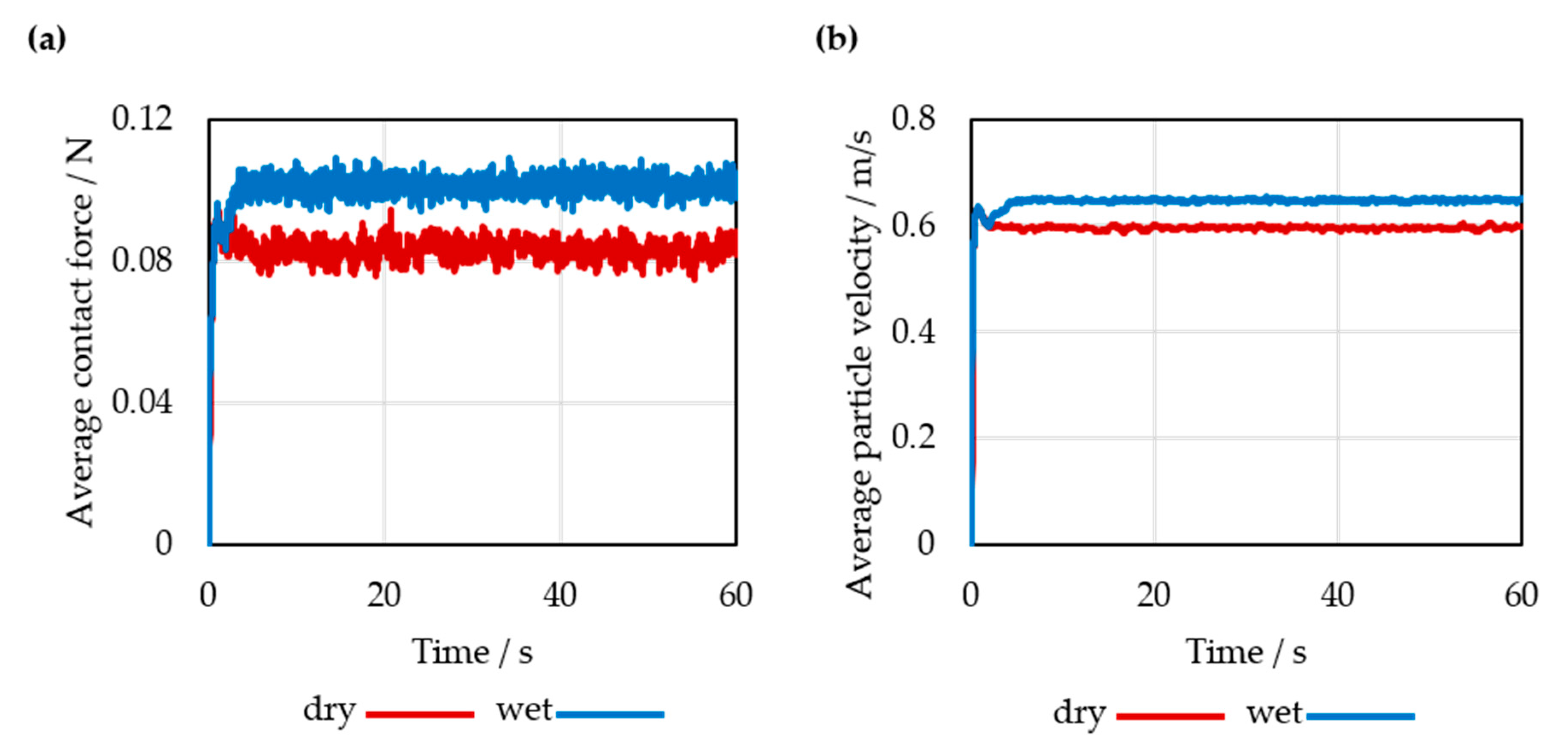
| Dry Case I | Water Injection Case II | Water Double Injection Case III | Water with Pharmacoat 606 Case IV | |
|---|---|---|---|---|
| Contact force (N) | 0.083 ± 0.007 | 0.101 ± 0.008 | 0.099 ± 0.006 | 0.148 ± 0.027 |
| Particle velocity (m/s) | 0.596 ± 0.003 | 0.647 ± 0.003 | 0.645 ± 0.003 | 0.647 ± 0.021 |
| Contact time (ms) | 0.058 ± 0.045 | 0.127 ± 0.007 | 0.165 ± 0.004 | 0.129 ± 0.005 |
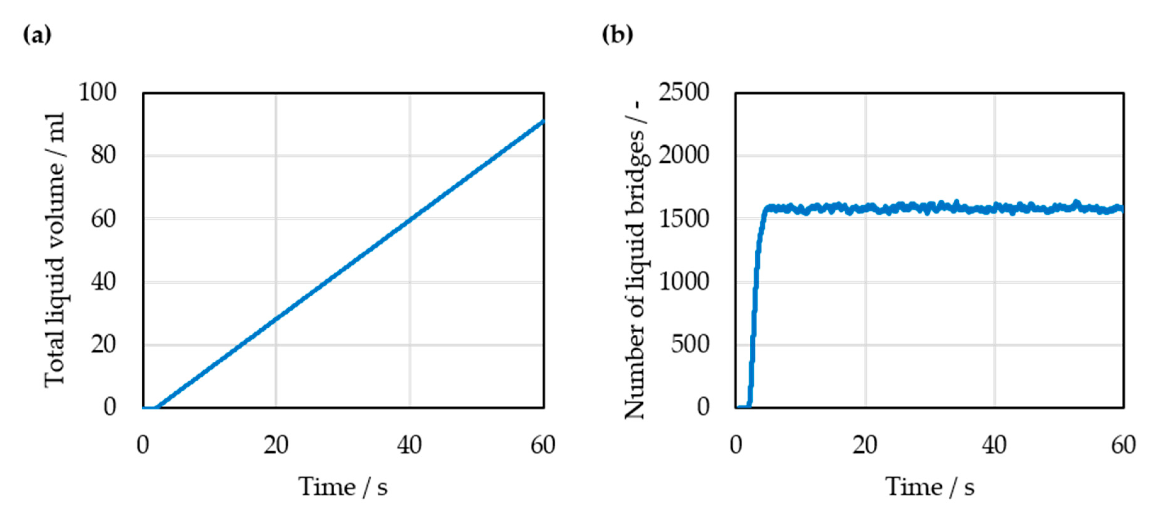
| Number of liquid bridges (-) | - | 1581 ± 85 | 1605 ± 91 | 1222 ± 82 |
© 2020 by the authors. Licensee MDPI, Basel, Switzerland. This article is an open access article distributed under the terms and conditions of the Creative Commons Attribution (CC BY) license (http://creativecommons.org/licenses/by/4.0/).
Share and Cite
Grohn, P.; Lawall, M.; Oesau, T.; Heinrich, S.; Antonyuk, S. CFD-DEM Simulation of a Coating Process in a Fluidized Bed Rotor Granulator. Processes 2020, 8, 1090. https://doi.org/10.3390/pr8091090
Grohn P, Lawall M, Oesau T, Heinrich S, Antonyuk S. CFD-DEM Simulation of a Coating Process in a Fluidized Bed Rotor Granulator. Processes. 2020; 8(9):1090. https://doi.org/10.3390/pr8091090
Chicago/Turabian StyleGrohn, Philipp, Marius Lawall, Tobias Oesau, Stefan Heinrich, and Sergiy Antonyuk. 2020. "CFD-DEM Simulation of a Coating Process in a Fluidized Bed Rotor Granulator" Processes 8, no. 9: 1090. https://doi.org/10.3390/pr8091090
APA StyleGrohn, P., Lawall, M., Oesau, T., Heinrich, S., & Antonyuk, S. (2020). CFD-DEM Simulation of a Coating Process in a Fluidized Bed Rotor Granulator. Processes, 8(9), 1090. https://doi.org/10.3390/pr8091090