Multi-Objective Optimization of Workshop Scheduling with Multiprocess Route Considering Logistics Intensity

Abstract

In order to solve the problems of flexible process route and workshop scheduling scheme changes frequently in the multi-variety small batch production mode, a multiprocess route scheduling optimization model with carbon emissions and cost as the multi-objective was established. At the same time, it is considered to optimize under the existing machine tool conditions in the workshop, then the theory of logistics intensity between equipment is introduced into the model. By designing efficient constraints to ensure reasonable processing logic, and then applying multilayer coding genetic algorithm to solve the case. The optimization results under single-target and multi-target conditions are contrasted and analyzed, so as to guide enterprises to choose a reasonable scheduling plan, improve the carbon efficiency of the production line, and save costs.

1. Introduction

Small and medium-sized enterprises often design different products in response to the changing needs of customers, so that a variety of small batch production models are formed from the limited production cycle and manufacturing resources. Many scholars have used a variety of methods to solve the optimization problems of energy saving, emission reduction, cost reduction, and time saving for the existing traditional manufacturing system, so that the green upgrade optimization of the system can be achieved without a large amount of investment [1,2,3,4,5,6,7,8,9]. It is worth mentioning that Li Congbo et al. [10] used the concept of feature elements and processing elements to establish a multi-objective machining route optimization model. Oleh et al. [11] built a process route planning model for complex and flexible workshop based on BOM (Bill of Material) tables. Liu et al. [12] planned route planning problem is transformed into a constrained traveling salesman problem, which was calculated using the ant colony algorithm. Fang et al. [13] proposed a mathematical programming model for the pipeline workshop scheduling problem considering peak power load, energy consumption, carbon emissions, and cycle time. Gonzalez et al. [14] proposed an effective neighborhood structure for flexible job shop scheduling problems, and realized the reassociation of discrete search process routes. Li Congbo et al. [15] considered job batch optimization and established multi-objective multiprocess flexible operation workshop scheduling model. Huang Xuewen et al. [16] established a multiprocess route scheduling model based on OR subgraphs, and proposed a new four-tuple mathematical description method to describe the process path and machine tool flexibility. Liu Qiong et al. [17] optimized the integrated process route a feature of the model with multiple parameters and mutual influence, a NSGA-II algorithm with four-stage coding was proposed.

Based on the existing research on such problems, this paper proposes a workshop scheduling optimization model with low carbon and low cost as the multi-objective. At the same time, in the optimization process of the existing research, the emergency task insertion, machine tools failure, and workpiece features are considered [18,19,20,21], but their combination with the actual situation of the equipment in the workshop needs to be supplemented. For this reason, this paper considers the impact of logistics strength between machine tools on optimization to guide the existing equipment, so as to help enterprises achieve the goal of effectively utilizing resources, reducing costs, reducing logistics movement, and improving operational efficiency.

In order to ensure reasonable processing logic, many scholars also made innovative research on the establishment of constraints. Zheng Yongqian et al. [22] introduced the feature constraint matrix and processing priority coefficient, and established the process ordering model of the machining center. Huang Yuyue et al. [23] considered the scheduling optimization of the shift time and other constraints in actual production. Yan Jungang et al. [24] proposed waiting dual time window constraints caused by limited time and equipment capabilities. An Xianghua [25] proposed the establishment of processing element constraints based on intuitionistic fuzzy numbers, and using the cellular automaton-SPEA2 multi-objective optimization algorithm. Chang Zhiyong et al. [26] established constraints of the geometric positional relationship between the features and used adaptive ant colony optimization algorithms to solve practical problems. Chunlong Li et al. [27] proposed a SEEHS constraint treatment method for hydropower plants based on feasible space and adopted a contrary adjustment method to deal with power balance constraints.

In order to solve problems, scholars also have their own ideas and innovations on algorithms. Nikhil Padhye et al. [28] propose a unified approach to improving different evolution. Kalyanmoy Deb et al. [29] proposed to improve the performance of particle swarm optimization by linking with the algorithm of genetic algorithm. De Jong et al. [30,31] introduced a new algorithm, an evolutionary algorithm, in detail. R. Čapek, P. et al. [32] proposed a heuristic algorithm based on priority construction with unscheduled steps and applied it to the case study of wire harness production. Gökan May et al. [33] reduced total energy consumption and processing time through a green genetic algorithm. Dunbing Tang et al. [34] used an improved particle swarm optimization algorithm to find the Pareto optimal solution of the dynamic flexible flow shop scheduling problem. Xiao-Ning Shen et al. [35] proposed an active response method based on multi-objective evolutionary algorithm (MOEA) for multiple targets such as efficiency and stability.

Based on the existing research, most of them take into account the influencing factors in the optimization process or consider the process route order to establish constraints. In this paper, some 0–1 variables are defined to constrain the processing sequence between processes and features, and ensure reasonable optimization and improve calculation efficiency.

2. Establishment of Multi-Objective Optimization Model for Process

Assumptions: (1) Features can select multiple process routes. (2) Processes in the process route are processed only once on one machine. (3) The machine tool will not malfunction regardless of inventory accumulation and part quality and volume.

The definitions $i’,j’,k’,l’$ are the previous part of the $i$th part, the previous machine of the $j$th machine tool, the previous feature of the $k$th feature, and the previous process route of the $l$th process route. The total processing time of a process of a feature of a part on the machine tool is $t_{ijk}$, the starting time is $s{t}_{ijk}$, and the part delivery time is ${\mathrm{ed}}_{\mathrm{i}}$.

Collection of parts $P={\{\mathrm{p}}_1,\cdots {,\mathrm{p}}_{\mathrm{i}},\cdots {,\mathrm{p}}_{\mathrm{a}}\text{}}$, $p_i$ indicates the $i$th of part, $i=1,2,\cdots ,a$.

Collection of machine tools $M={\{\mathrm{m}}_1,\cdots {,\mathrm{m}}_{\mathrm{j}},\cdots {,\mathrm{m}}_{\mathrm{b}}\text{}}$, $m_j$ indicates the $j$th of machine tool, $j=1,2,\cdots ,b$.

Collection of features for all parts $OP={\{\mathrm{op}}_1,\cdots {,\mathrm{op}}_{\mathrm{i}},\cdots {,\mathrm{op}}_{\mathrm{a}}\text{}}$, $o{p}_i$ indicates the $i$th of part’s all features.

The collection of features for each part ${\mathrm{op}}_{\mathrm{i}}={\{\mathrm{op}}_{\mathrm{i}1},\cdots {,\mathrm{op}}_{\mathrm{ik}},\cdots {,\mathrm{op}}_{\mathrm{ic}}\text{}}$, $o{p}_{ik}$ indicates the $i$th of part’s the $k$th of feature, $k=1,2,\cdots ,c$. Defining variables ${\chi }_{\mathrm{ik}}\in \{0,1\text{}}$, which means whether the feature $o{p}_{ik’}$ of the $i$th of part needs to be machined before the feature $o{p}_{ik}$, if necessary ${\chi }_{ik}=1$; otherwise, it is zero.

The collection of process routes selectable for each feature is $OPR={\{\mathrm{opr}}_{\mathrm{ik}1},\cdots {,\mathrm{opr}}_{\mathrm{ikl}},\cdots {,\mathrm{opr}}_{\mathrm{ikd}}\text{}}$, $op{r}_{ikl}$ indicates that the $k$th feature of the $i$th part selects the $l$th process route for processing, $l=1,2,\cdots ,d$.

The collection $OPM={\{\mathrm{opm}}_{\mathrm{ikl}1},\cdots ,{\mathrm{opr}}_{\mathrm{iklj}},\cdots {,\mathrm{opr}}_{\mathrm{iklb}}\text{}}$ represents the process included in the routing (corresponding machine tool), and $op{\mathrm{m}}_{iklj}$ represents the $k$th feature of the $i$th part selected the $l$th process route and processed by the $j$th machine tool. The variable ${\iota }_{\mathrm{iklj}}\in \{0,1\text{}}$ is defined, which means whether the previous process $op{\mathrm{m}}_{iklj’}$ of process route $l$ needs to be completed before $op{\mathrm{m}}_{iklj}$, if necessary ${\iota }_{iklj}=1$; otherwise, it is zero.

2.1. The Model of Carbon Emission

When the CNC machine is in the standby or preparation stage, the standby power of the machine $P_1$ consists of the power-related auxiliary system, the motor, and the servo. The waiting time before the machining and the input program is $t_1$; when a machine tool is processing different parts, the tool needs to be adjusted more; the tool setting time is $t_2$, the movement time of the X, Y and Z axes of the machine tool are $t_{X_1},t_{Y_1},t_{Z_1}$, the moving power of each axis is $P_{X_1},P_{Y_1},P_{Z_1}$, and the power is 0 if no movement occurs (such as the spindle of the lathe); when the spindle Z starts to rotate, the no-load rotary power is $P_{Z_2}$, the no-load standby power is $P_{\mathrm{s}}=P_1+P_{Z_2}$, and the no-load standby time is $t_{\mathrm{s}}$, then the $k$th feature of the $i$th part before the $j$th machine tool starts processing and can be expressed as

$$E_{ijk}^s=P_1\cdot t_1+P_1\cdot t_2+P_{X_1}\cdot {\mathrm{t}}_{X_1}+P_{Y_1}\cdot {\mathrm{t}}_{Y_1}+P_{Z_1}\cdot {\mathrm{t}}_{Z_1}+P_{\mathrm{s}}\cdot t_{\mathrm{s}}$$

(1)

$$t_2={\mathrm{t}}_{X_1}+{\mathrm{t}}_{Y_1}+{\mathrm{t}}_{Z_1}$$

(2)

The cutting process of each procedure includes the air-cut energy $E_{ijk}^{air}$ and cutting energy $E_{ijk}^m$. The air-cut energy consumption of the machine tool includes the power of the X and Y axes of the machine tool. The power of each axis is $P_X,P_Y$, and the energy consumption generated during the moving time is $t_{X_2},t_{Y_2}$. If the spindle has movement (such as milling machine, grinding machine, etc.), the moving power $P_{Z_2}$ of the spindle Z generates energy consumption in time $t_{Z_2}$. And the energy consumption of the no-load and standby parts of the machine during the air-cut time need to be considered. The cutting energy consumption is the energy consumed by the machine tool in the cutting time $t_m$. For different machine tools and different cutting three-factor machine power, the actual machining power $P_{ijk}$ of each process is measured. Therefore, the $k$th feature of the $i$th part is machined on the $j$th machine tool can be expressed as

$$E_{ijk}^{air}+E_{ijk}^m=P_X\cdot {\mathrm{t}}_{X_2}+P_Y\cdot {\mathrm{t}}_{Y_2}+P_{Z_2}\cdot {\mathrm{t}}_{Z_2}+P_{\mathrm{s}}\cdot (t_{X_2}+t_{Y_2}+t_{Z_2})+P_{ijk}\cdot t_m$$

(3)

The auxiliary system energy consumption includes the energy consumed by the power $P_c$ such as the filtration and cooling system during the cutting time $t_m$; the energy consumption generated during the standby time $t_{\mathrm{chp}}$ of the machine during the loading and unloading of the parts; after machining $N$ times on the $j$th machine tool, the tool needs to be replaced. The energy consumption of the machine tool standby during the tool change time $t_{\mathrm{cht}}$, the auxiliary energy consumption of the the $k$th feature of the $i$th part is machined on the $j$th machine tool can be expressed as

$$E_{\mathrm{ijk}}^{\mathrm{as}}=P_c\cdot t_m+P_1\cdot t_{\mathrm{chp}}+\frac{P_1\cdot t_{\mathrm{cht}}}{N}$$

(4)

Taking energy consumption as the basic input and greenhouse gas (GHG) as the output, the corresponding carbon emissions in this process are converted through the carbon emission coefficient of various energies [36]. $\xi$ is the carbon emission coefficient of energy (fuel, electricity, etc.), and taking into account the environmental (regional and time) impact factors $\delta$ and auxiliary process influence factors $\mu$, the carbon emissions can be defined as

$$W=\xi (1+\delta +\mu )E$$

(5)

The carbon emissions for cutting in each process can be expressed as

$$W_{ijk}=\xi (1+\delta +\mu )\cdot (E_{ijk}^s+E_{ijk}^{air}+E_{ijk}^m+E_{ijk}^{as})$$

(6)

It is assumed that no more than one machine is used for each process of the part; the collection of carbon emissions from part processing can be expressed as $W=\{W_{111}\cdots W_{ijk}\cdots W_{abc}\}$, where $W_{ijk}$ indicates the processing carbon emission of the $k$th feature of the $i$th part that was machined on the $j$th machine tool.

2.2. The Model of Cost

The processing cost of parts increases with the increase of processing time. It is divided into three aspects: machine tool cost, loss cost, and ancillary costs. Machine tool costs include energy consumption costs during standby, air cutting, cutting operations, etc. The expression for each process is

$$\begin{array}{l}{C}_{ijk}^m=M_e\times t_{ijk},\\ t_{ijk}=t_1+t_2+t_{X_1}+t_{Y_1}+t_{Z_1}+t_{X_2}+t_{Y_2}+t_{Z_2}+t_s+t_m+t_{chp}+\frac{t_{cht}}{N},\end{array}$$

(7)

where $C_{ijk}^m$ is the processing cost (US$) for each process and $M_e$ is the unit cost (US$/s). $t_{ijk}$ (s) is the total processing time of the part, which includes all the time associated with processing.

The loss cost includes the grinding wheel loss and the cutting fluid consumption. During the processing of N procedures, multiple tool dressings are required until the tool is worn to the minimum size and scrapped. The consumption of the cutting fluid is composed of the part where the temperature of the surface rises to evaporate the cutting fluid into the air, the part taken away by the chips, and the part deposited on the surface of the part. The loss cost $C_{ijk}^{loss}$ (US$) generated by each process is

$$C_{ijk}^{loss}=\frac{M_a+M_l\times L}{N}$$

(8)

where $M_a$ is the tool cost (US$), $L$ is the amount of cutting fluid (L) added during $N$ times processes, and $M_l$ is the cutting fluid cost (US$/L).

The ancillary cost includes labor costs, which is the labor remuneration paid by workers during the process, and also includes the operating costs of each process, which include the costs of lubricants, water, equipment maintenance, and repair. Then, each process ancillary cost $C_{ijk}^{as}$ (US$) is

$$C_{ijk}^{as}=(M_p+M_u)\times t_{ijk}$$

(9)

where $M_p$ is labor cost (US$/s) and $M_u$ is operating cost (US$/s).

Then, the cost of each processing operation is

$$C_{ijk}=C_{ijk}^m+C_{ijk}^{loss}+C_{ijk}^{as}$$

(10)

Collection of parts cost can be obtained as $C=\{C_{111}\cdots C_{ijk}\cdots C_{abc}\}$; $C_{ijk}$ indicates the processing cost of the $k$th feature of the $i$th part that was machined on the $j$th machine tool.

2.3. Optimization Model Considering Logistics Strength

The system layout design of System Layout Planning (SLP) is the method used by the manufacturing enterprise in equipment planning [37]. The functions that the production system should perform include the system design and planning of the equipment, personnel, logistics, and investment within the system. The core content is based on the analysis of factory production logistics, combined with the degree of interconnection of operating units, and then the design and plan of the location of the production equipment.

To carry out workshop scheduling via the multiprocess route in manufacturing enterprises, the machine tool equipment has been relatively fixed, so it should be considered to carry out multi-objective optimization in the existing equipment planning and logistics system. We analyzed the logistics and other elements of the production line:

(1)

Under the cluster layout, a temporary storage area is set between two areas or near the processing machine to facilitate the overall transportation of parts. The evaluation coefficient of the storage area is defined as $A_{\mathrm{j}’\mathrm{j}}$. When it is necessary to use the storage area to store parts, the value of the coefficient is bigger, and vice versa.

(2)

The transportation of parts will occur between the production areas or the machine tools. The material flow evaluation coefficient between the two processes connected is defined as $B_{\mathrm{j}’\mathrm{j}}$. The more numerous and heavier the parts that need to be transported between the processes are, the greater the value of the coefficient, and vice versa.

(3)

The layout position of the machine tool determines the length of the logistics route. The distance evaluation coefficient between two processes connected is defined as $C_{\mathrm{j}’\mathrm{j}}$. The longer the distance between the processes, the greater the value of the coefficient, and vice versa.

(4)

There is a difference in the logistics frequency between processes. We define the logistics frequency evaluation coefficient between the two processes as $D_{\mathrm{j}’\mathrm{j}}$. The higher the frequency of transportation between machine tools, the greater the value of the coefficient, and vice versa.

(5)

We analyzed the environmental conditions between the areas or the machine tools, defining the conversion evaluation coefficient as $I_{\mathrm{j}’\mathrm{j}}$. When the logistics environment is more complicated, the value of the coefficient is greater, and vice versa.

In summary, the logistics intensity evaluation function between two machine tools is established, and the expression is

$$L{O}_{j^{\prime }j}=A_{j^{\prime }j}{B}_{j^{\prime }j}{C}_{j^{\prime }j}{D}_{j^{\prime }j}{I}_{j^{\prime }j}$$

(11)

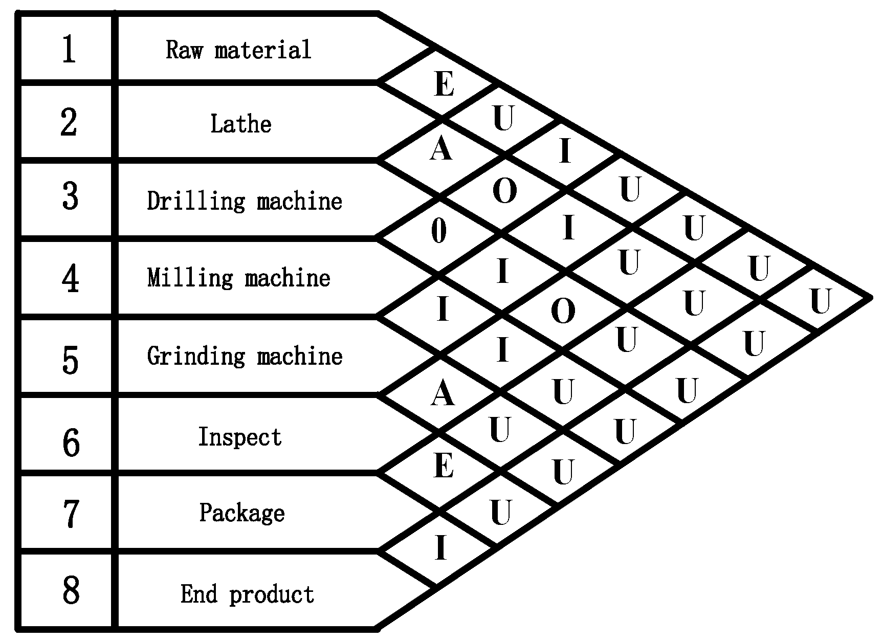
According to the actual situation of the enterprise’s production line, define the evaluation indicators of each coefficient. The logistics information in the factory can be collected, and substituted into Formula (11) to be calculated, to then obtain the logistics strength evaluation function $L{O}_{j^{\prime }j}$. The range is divided into five levels, so that the logistics intensity between machine tools is divided into intensity levels (A, E, I, O, U). Based on score, the logistics priority coefficient $G_{\mathrm{j}’\mathrm{j}}$ can be established to define the logistics strength of the machine tool j’ to the machine tool j. The intensity level can converted into a natural number of 0–4; the smaller the value, the higher the logistics intensity between processes. The unit logistics related table can be drawn, as shown in Figure 1.

Combined with the analysis of logistics, we can get a collection of logistics strength between machine tools $G=\{G_{11}\cdots G_{j’j}\cdots C_{b’b}\}$.

The definition of the independent variable ${\gamma }_{ikl}\in \{0,1\}$ indicates whether the routing $op{r}_{ikl}$ is selected, and if the $l$th route of the $k$th feature is selected ${\gamma }_{ikl}=1$; otherwise, it is zero.

The objective function can be obtained according to the carbon emission and cost of the machine tool processing corresponding to the selected process route, and the logistics strength between the machine tools used in the process of the preceding and following process routes,

$$\min ({\displaystyle \sum G_{j’j}\cdot } {\gamma }_{ikl}\cdot W_{ijk}, {\displaystyle \sum G_{j’j}\cdot {\gamma }_{ikl}\cdot C_{ijk}})$$

s.t.

$$s{t}_{ij’k}+t_{ij’k}+Q(1-{\gamma }_{ikl})<{\chi }_{ik}{\iota }_{\mathrm{iklj}}s{t}_{ijk},\hspace{1em}\forall i,j,j’,k$$

(12)

$$s{t}_{ijk}-s{t}_{i’jk’}>t_{i’jk’}+Q(1-{\gamma }_{ikl}),\hspace{1em}\forall i,i’,j,k,k’$$

(13)

$${\displaystyle \sum _l^d{\gamma }_{ikl}=1}, \hspace{1em}\forall i,k,l$$

(14)

$$s{t}_{ij’k}\ge 0,\hspace{1em}\forall i,j’,k$$

(15)

$$\max (s{t}_{ijk}+t_{ijk})\le e{d}_i,\hspace{1em}\forall i,j’,k$$

(16)

where Q is a maximum value, and Formula (12) indicates that the process route satisfies the processing order between the features and the order of processing between processes; Formula (13) means that one machine can only process one part at a time; Formula (14) means that one feature of a part can only select one process route; Formula (15) indicates that the part processing should start from time 0; Formula (16) indicates that the last process of the part needs to be completed before the part delivery date.

3. Multilayer Coding Genetic Algorithm

The multilayer coding genetic algorithm divides the individual coding into multiple layers; each layer of coding contains different meanings, and jointly expresses the complete solution of the problem, thereby using a chromosome to accurately express the solution of the complex problem.

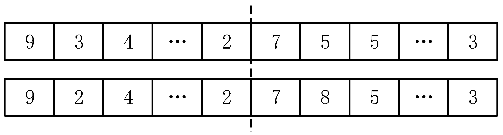
First, the constraint type of the optimization problem is determined, the solution set of the population composition problem is initialized, and an extended process-based coding is designed. Each chromosome represents a feasible solution under the target optimization. There are multiple kinds of products to be processed in this paper. When the product $n_i$ has $m_j$ processes, the individual lengths of the chromosomes have a total of $2{\displaystyle \sum _{i=1}^k{n}_i}{m}_j$ integers, where in the first half is the processing order of the product features on the machine, and the second half represents the machine tool corresponding to the selected machining method. As shown in Figure 2, if the second feature can be processed by a third or second machining method, the corresponding machine tools are 5 and 8.

To determine the fitness value of a chromosome, it is necessary to reduce the chromosome into a process. It is also necessary to consider the logistics strength of the machine tool used in the current process and the machine tool used in the previous process, and also to consider how the target allocates the ratio of the processed carbon emissions and the processing cost in the multi-objective optimization. Forming a fitness calculation function, the calculation formula is

$$fitness(i)=k_1\cdot W_{ijk}\cdot G_{j’j}+k_2\cdot C_{ijk}\cdot G_{j’j}$$

(17)

where $k_1,k_2$ are the coefficients, the smaller the total carbon emissions and cost generated by the process route of all parts, the better the chromosome.

The roulette method is used to select chromosomes with good fitness. The probability that chromosome $i$ is selected every time is $p(i)$. The better the chromosome is, the smaller the fitness value is. If the value is larger after derivative, the selected probability will be greater.

$$p(i)=Fitness(i)/{\displaystyle \sum _{i=1}^{n}Fitness(i)}$$

(18)

$$Fitness(i)=1/fitness(i)$$

(19)

The crossover of the integer crossover method is used to obtain new chromosomes, and the population is continuously evolved. Two chromosomes are selected from the population by roulette method, the ${\displaystyle \sum _{\mathrm{i}=1}^{\mathrm{k}}{n}_i{m}_j}$ bits are selected from the individual codes, and the intersection positions are randomly selected for intersection. After the intersection, the process in each process route will be redundant or missing, and the excess part of the process will be added to the missing part. It is judged whether the process conforms to the processing logic according to the constraint conditions. Then, the processing machine corresponding to each process is adjusted to a machine tool of ${\displaystyle \sum _{\mathrm{i}=1}^{\mathrm{k}}{n}_i{m}_j}+1$ to $2{\displaystyle \sum _{\mathrm{i}=1}^{\mathrm{k}}{n}_i{m}_j}$ position.

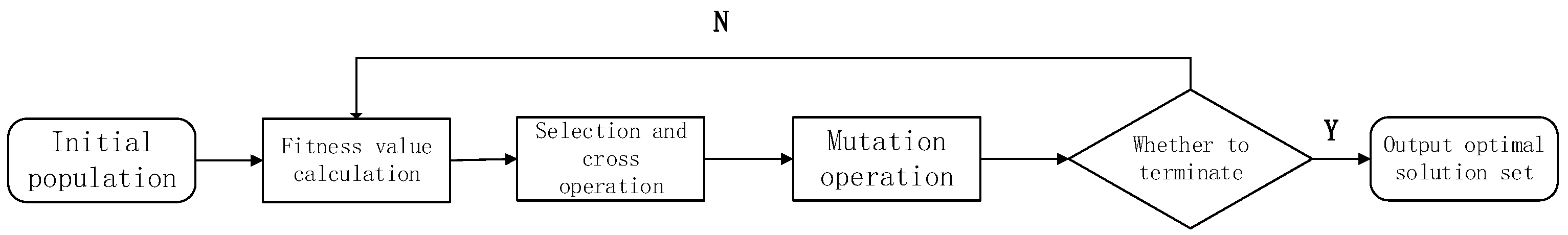
Integer variation is used to obtain excellent individuals and promote the evolution of the entire population. The chromosomes are randomly selected from the population, the first half of the individual is selected to perform the mutation operation, and the machine tool corresponding to the second half is exchanged. The entire algorithm process is shown in Figure 3.

4. Examples and Analysis

According to the production situation of an air compressor crankshaft of a commercial vehicle brake system company, a processing example can be fitted. In this example, set the part set $P$, that is, process eight kinds of parts at the same time on a production line. Any part contains three major features and the available feature set $OP$. Any feature has multiple process routes that can be selected and the available process route set $OPR$. The number of the machine tools in the workshop form a set $M$, that is, the production line has a total of 15 selectable processing machine tools, including machine tools with the same processing method but different numbers. Comprehensively considering the machine tool set and the process route set, the process set $OPM$ can be obtained.

The machine tool can be selected according to the features’ process route.

Table 1. Parts’ features selectable machine tools.

Part	Feature1			Feature2			Feature3
1	5	12	4	[2,15]	[3,8]	5	[9,11]	0
2	4	[2,15]	8	[6,10]	5	[1,12]	3	[2,15]
3	1	[6,10]	13	[2,15]	[7,14]	5	[9,11]	[3,8]
4	5	15	[7,14]	10	[2,15]	[3,8]	0	0
5	[7,14]	5	[9,11]	11	2	[3,8]	[1,12]	[2,15]
6	[6,10]	4	[11,9]	14	8	[3,8]	7	[7,14]
7	1	[6,10]	10	[2,15]	[2,15]	5	[1,12]	0
8	11	[7,14]	15	[2,15]	5	7	[1,12]	9

expresses the optional machine matrix $J_{\mathrm{m}}$, which longitudinally represent eight parts, horizontally represent the machine tool corresponding to the features of the parts, and the brackets indicate the various machine tools that can be selected; 0 means no such process. For example, the processing route of part 1 includes 5-12-4-2-3-5-9, 5-12-4-2-8-5-9, 5-12-4-2-8-5-11, 5-12-4-2-3-5-11, 5-12-4-15-3-5-9, 5-12-4-15-8-5-9, 5-12-4-15-8-5-9, 5-12-4-15-8-5-11, and 5-12-4-15-3-5-11; there are a total of eight process routes.

Similar to the optional machine tool matrix $J_{\mathrm{m}}$, a processing time matrix $T$ is generated based on the machining time of the part features on the machine, as shown in

Table 2. Parts’ features processing time.

Part	Feature1			Feature2			Feature3
1	3	10	9	[5,4]	[5,3]	10	[5,7]	0
2	6	[8,6]	4	[5,6]	3	[3,3]	6	[2,3]
3	4	[5,7]	7	[5,5]	[9,11]	5	[8,5]	[4,3]
4	7	3	[4,6]	3	[5,7]	[3,6]	0	0
5	[6,4]	10	[7,9]	8	5	[4,7]	[4,6]	[5,6]
6	[3,5]	10	[8,7]	9	4	[9,4]	5	[4,6]
7	6	7	9	[8,7]	[4,5]	3	[5,5]	0
8	8	[6,7]	5	[10,8]	6	4	[7,5]	7

.

Set the logistics strength matrix $G_{J\mathrm{m}}$ of 15 machine tools according to the collection of logistics strength $G$,

$$G_{J\mathrm{m}}=\left[\begin{array}{cccccccc}& 1& 2& 3& \cdots & 13& 14& 15\\ 1& 0& 4& 2& & 4& 4& 2\\ 2& 4& 0& 1& \cdots & 3& 4& 3\\ 3& 2& 1& 0& & 4& 3& 2\\ ⋮& & ⋮& & \ddots & & ⋮& \\ 13& 4& 3& 4& & 0& 2& 1\\ 14& 4& 4& 3& \cdots & 2& 0& 1\\ 15& 2& 3& 2& & 1& 1& 0\end{array}\right]$$

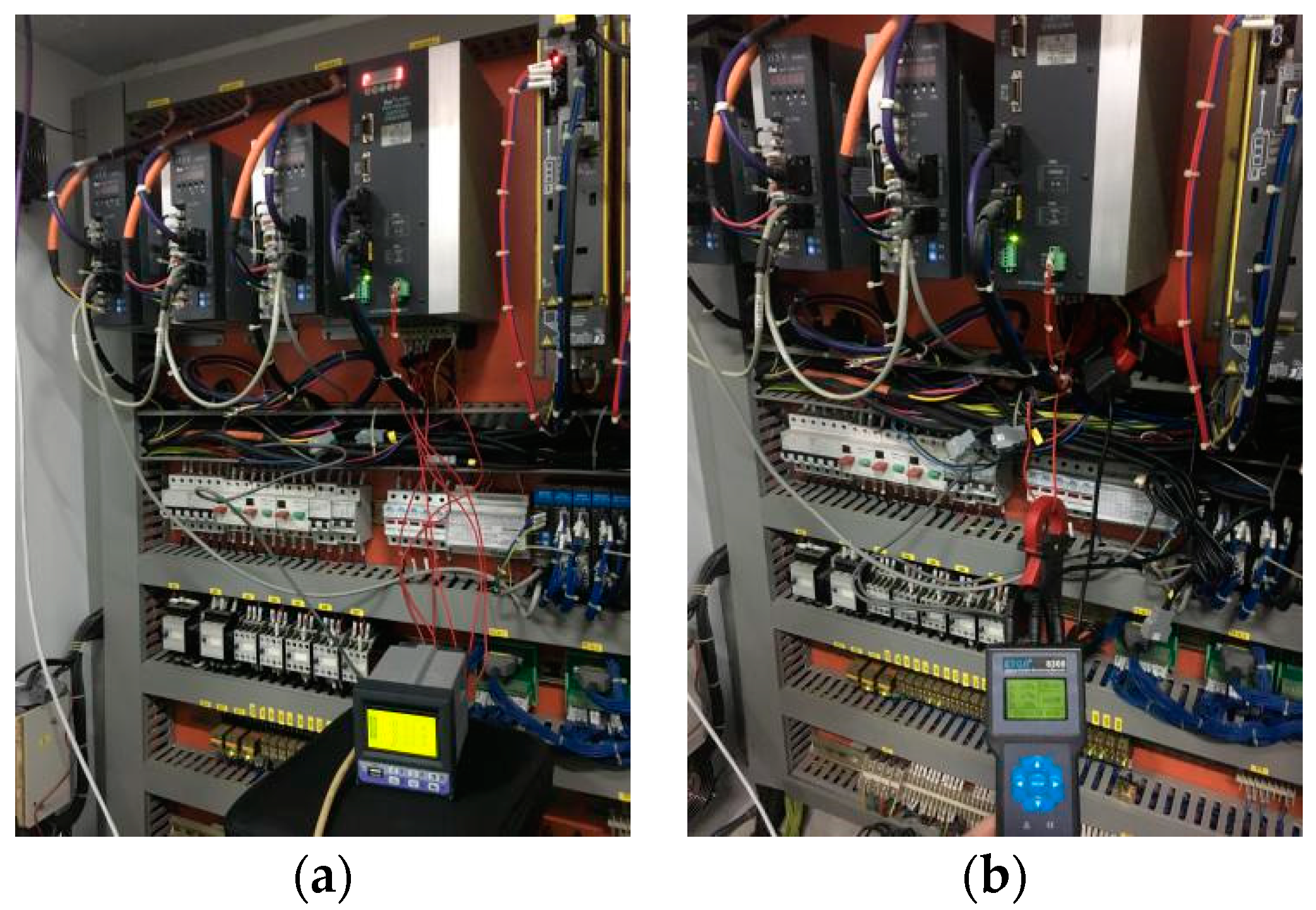
In order to complete the calculation of the model, the power value of each machine tool in the carbon emission model needs to be collected, and the control equipment enters the processing stages of standby and empty cutting. We used the three-phase four-wire connection method to connect the power recorder to the motor used in each stage. The control equipment works stably and collects the corresponding power value. The data is substituted into the expressions of the model. At the same time, the current monitoring device can be connected to the device to monitor the current situation at various stages of stable operation, and the accuracy of the power value can be reversed to improve the accuracy of the data [5]. The connection of the power recorder is shown in Figure 4a, and the connection of the current monitoring device is shown in Figure 4b.

Using the power detection experimental method and the timing of the processing process, the carbon emissions $W_{ijk}$ and processing costs $C_{ijk}$ of each machine tool during processing can be calculated. Then, the carbon emission matrix W and processing cost matrix C can be determined, which are similar to the optional machine tool matrix $J_{\mathrm{m}}$ and processing time matrix $T$.

Substituting five matrices into the algorithm calculation, the number of populations is 40, the maximum number of iterations is 50, the crossover probability is 0.8, and the mutation probability is 0.6.

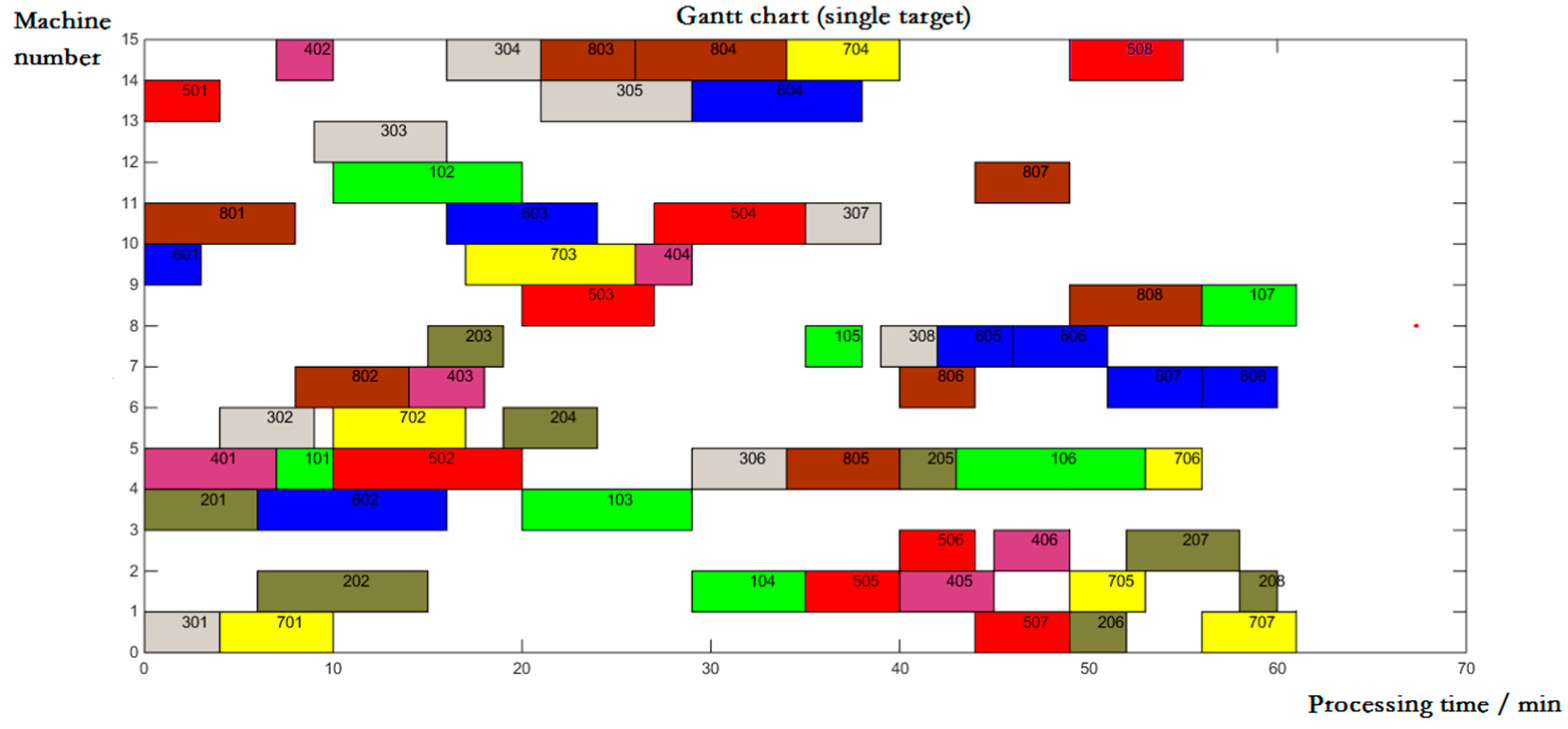
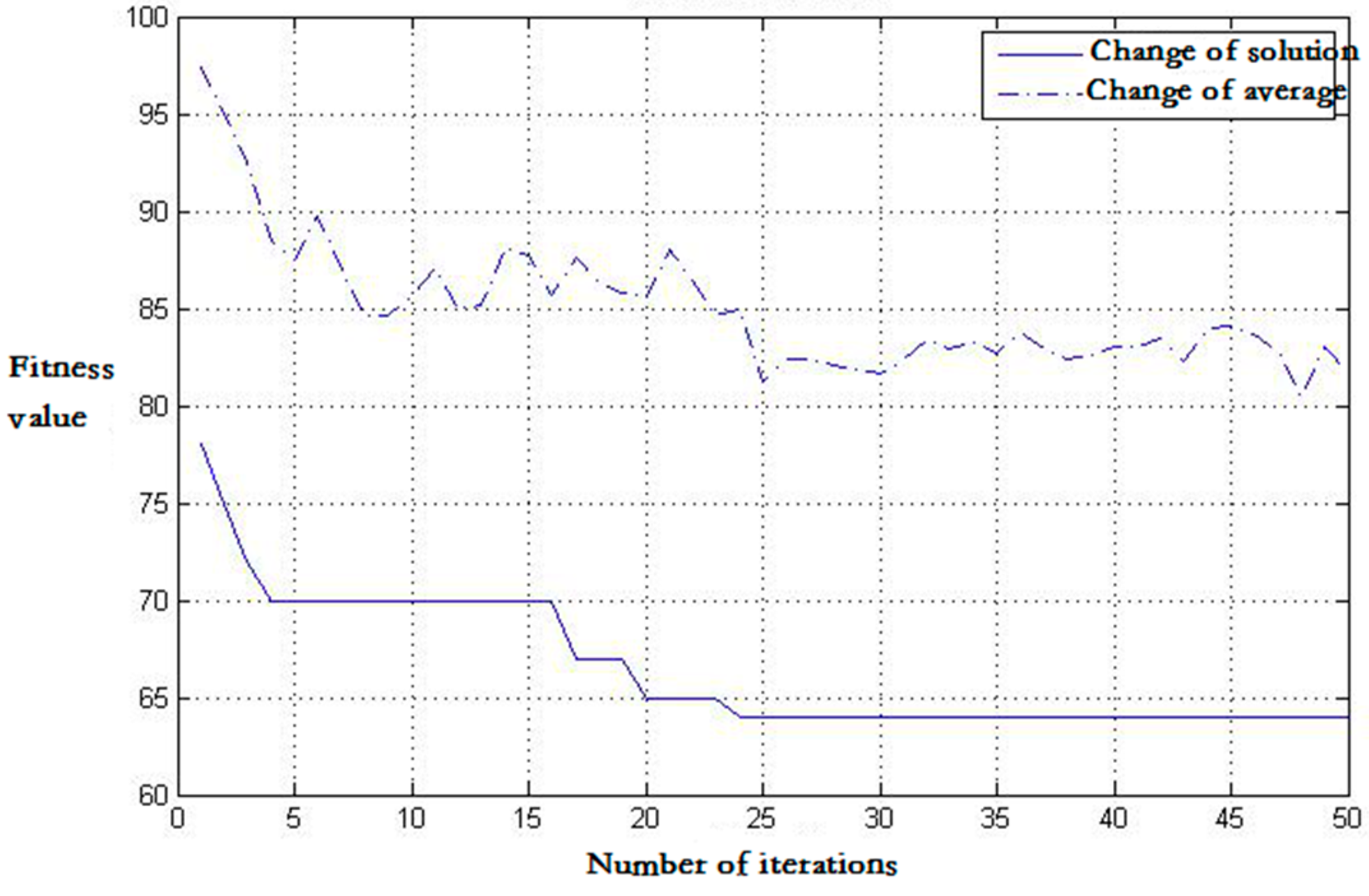
When the cost is optimized separately, the algorithm is iterated for 24 generations. The results are shown in Figure 5 and Figure 6. The completion time is 61 min and the carbon emission is 28.8 Kg. Each part feature mainly considers selecting a machine tool with a short machining time. The process route selects a route with less machine conflict and expands the parallel machining, which reduces the waiting time of the workpiece and reduces the maximum completion time.

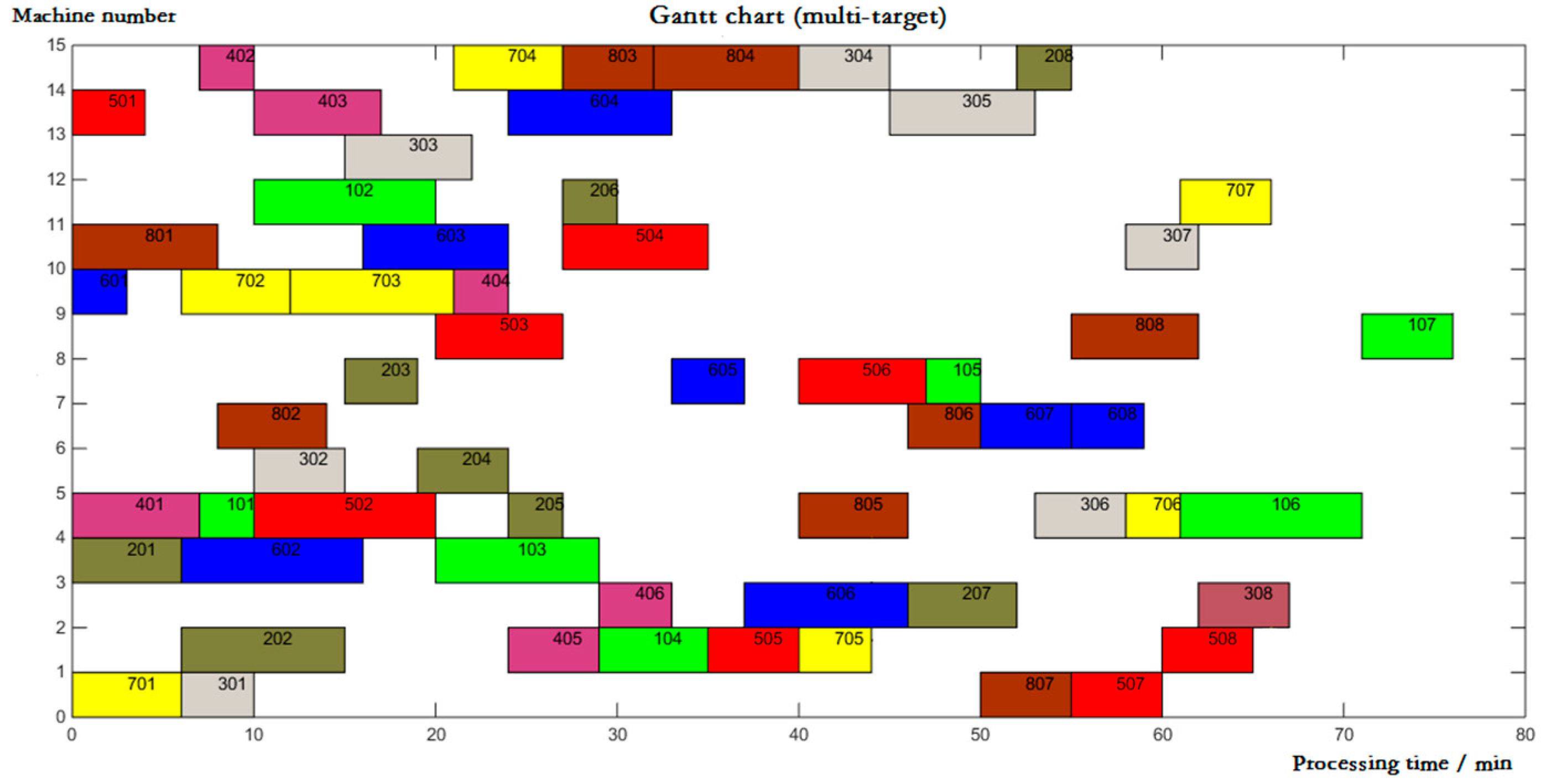
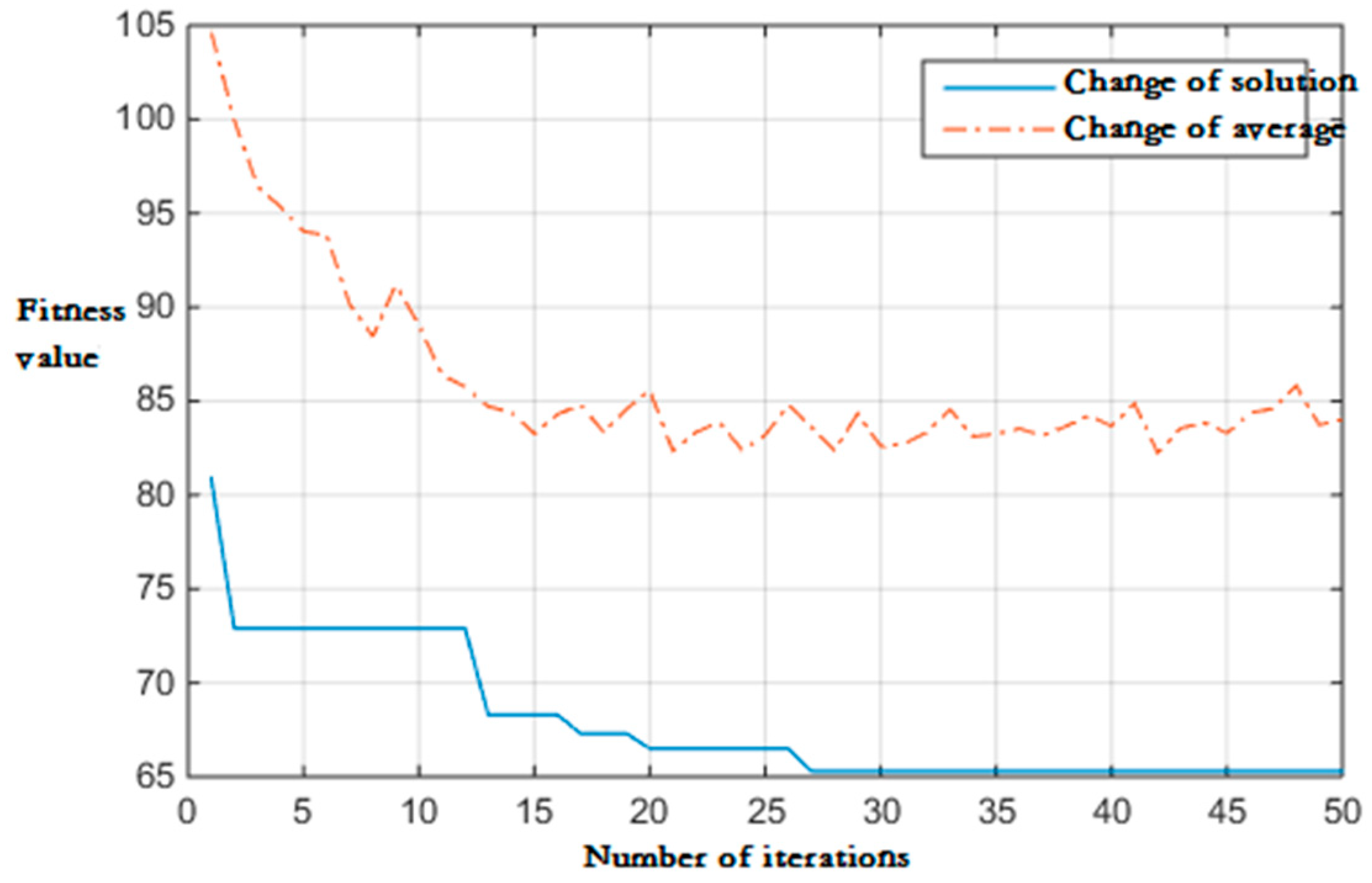
When increasing carbon emissions for multi-objective optimization, the fitness coefficients k1 and k2 are taken as 0.5 and 0.5, respectively, and the algorithm is iterated for 27 generations. The results are shown in Figure 7 and Figure 8. The total carbon emissions of the workshop are 23.7 Kg, which is 17.7% lower than the cost optimization alone. Most of the characteristics of each part will choose the processing route with less carbon emission and its corresponding machine tool for processing, which reduces the total carbon emission. However, the concentration of processing machine tools leads to the increase of waiting time in the process. The time has increased by 15 min and the cost has also increased.

5. Conclusions

This paper establishes a multiprocess route workshop scheduling optimization model with the lowest carbon emissions and the best cost by defining a set of factors that affect machining production. At the same time, in order to make the model accurately fit the actual facility conditions, the existing equipment and the factors that affect the logistics intensity are also analyzed. The evaluation coefficients and functions are defined, and the logistics intensity model is fitted and substituted into the objective function. The scheduling modeling and optimization process of the production line has certain reference value. Considering the actual conditions, such as the processing order between the parts’ features and the processing order between processes, 0–1 variables $\chi$, $\gamma$, and $\tau$ are introduced to ensure that the optimization process meets the actual processing order. Finally, through the fitting processing example, the multilayer coding genetic algorithm was used to calculate the Gantt chart under single-objective and multi-objective optimization, and the conclusion was drawn through comparative analysis, which verified the practicability and accuracy of the model, thus guiding the multi-objective. The process of workshop scheduling optimization for small and large batch parts manufacturing enterprises is defined. However, the modeling does not take into account the production line dynamics such as machine tool equipment sudden failures and order changes, and ignores the impact of peak power and processing quality, so optimization research needs to be further in-depth.