Article

Kinetic Parameter Determination for Depolymerization of Biomass by Inverse Modeling and Metaheuristics

by
Dalyndha Aztatzi-Pluma
1,2,
Susana Figueroa-Gerstenmaier
1,
Luis Carlos Padierna
1,*,
Edgar Vázquez-Núñez
1 and
Carlos E. Molina-Guerrero
1,*
1
Department of Chemical, Electronics and Biomedical Engineering, University of Guanajuato, Lomas del Bosque 103, Lomas del Campestre, Leon, Guanajuato 37150, Mexico
2
Tecnologico Nacional de Mexico/Instituto Tecnologico Superior de Abasolo, Cuitzeo de los Naranjos 401, Abasolo, Guanajuato 37150, Mexico
*
Authors to whom correspondence should be addressed.
Processes 2020, 8(7), 836; https://doi.org/10.3390/pr8070836
Submission received: 28 May 2020 / Revised: 10 July 2020 / Accepted: 11 July 2020 / Published: 14 July 2020
(This article belongs to the Special Issue Optimization Algorithms Applied to Sustainable Production Processes)

Abstract

:
A computational methodology based on inverse modeling and metaheuristics is presented for determining the best parameters of kinetic models aimed to predict the behavior of biomass depolymerization processes during size scaling up. The Univariate Marginal Distribution algorithm, particle swarm optimization, and Interior-Point algorithm were applied to obtain the values of the kinetic parameters (KM and Vmax) of four mathematical models based on the Michaelis–Menten equation: (i) Traditional Michaelis–Menten, (ii) non-competitive inhibition, (iii) competitive inhibition, and (iv) substrate inhibition. The kinetic data were obtained from our own experimentation in micro-scale. The parameters obtained from an optimized micro-scale experiment were compared with a bench scale experiment (0.5 L). Regarding the metaheuristic optimizers, it is concluded that the Interior-Point algorithm is effective in solving inverse modeling problems and has the best prediction power. According to the results, the Traditional model adequately describes the micro-scale experiments. It was found that the Traditional model with optimized parameters was able to predict the behavior of the depolymerization process during size scaling up. The methodology followed in this study can be adopted as a starting point for the solution of future inverse modeling problems.

1. Introduction

Vegetal biomass (VB) is an alternative for biofuel production. VB is mainly composed of cellulose, hemicellulose, and lignin and can be transformed into different products through four fundamental stages: (i) conditioning, (ii) depolymerization or enzymatic hydrolysis, (iii) fermentation, and (iv) the downstream process [1,2]. In this context, the depolymerization stage is the most expensive, and predicting the reaction behavior is essential to achieve a higher reaction yield. One of the most widely used models to describe the behavior of this phenomenon is the Michaelis–Menten (M–M) equation. The M–M equation consists of two parameters: the Michaelis constant (KM) and the maximum reaction velocity (Vmax), which describe the speed of the enzymatic reactions related to the reaction rate (rs) and the concentration of a substrate (S), as described in Equation (1) [3].
r s = d S d t = V m a x × S K M + S
The determination of these parameters (Vmax and KM) allows one to predict the behavior of the depolymerization reaction. This equation has been used to follow various enzymatic reactions, e.g., hydrolysis of proteins, biomass, and even the elimination or interaction of drugs in the human body [2,3,4]. A methodology that can be followed to obtain these parameters is inverse modeling (IM) supported by computational intelligence (CI) methods. On the one hand, IM consists of estimating the parameters in a mathematical model from measured observations [5]. This type of estimation begins with comprehensive data at the level of intact systems. It leads to inferences of parameter values at lower levels of organization—namely, features of individual processes. Thus, it is called “top-down” or “inverse” [6].
On the other hand, CI can be defined as a set of nature-inspired computational models that comprehend the subfields of fuzzy logic, artificial neural networks, and evolutionary algorithms. These models are designed to address real-world problems of prediction, control, classification, optimization, and other tasks [7]. Optimization methods of CI, also known and hereafter referred to as metaheuristics, have been successfully applied to identify a vast number of nonlinear dynamic systems [8] and parameter estimations and facilitate the structure identification of biochemical systems [6]. To address the IM, not only metaheuristics (such as genetic algorithms, simulated annealing particle swarm optimization (PSO), or Estimation of Distribution algorithms (EDAs) but also other algorithms for specific biochemical systems (such as alternating regression, eigenvector optimization, and dynamic flux estimation) have been applied [6]. Among the available methods, EDAs and PSO have been recently studied for biochemical parameter estimation and have shown to be optimal algorithms for some hyper-parameter tuning applications [9,10].
In the biofuel area, depolymerization experiments are developed at the flask level, evaluating multiple parameters resulting in large assay experiments with intensive requirements. To reduce these intensive requirements and enable the evaluation of numerous parameters, micro-scale experiments have been proposed as an alternative tool to optimize some aspects of bioprocesses (e.g., biomass depolymerization) [11]. In addition, few reports have been published on an assay of the depolymerization process at a micro-scale [11,12,13]. This may be because the methodology has not been validated as a tool that can predict the behavior of depolymerization at larger scales.
Given the high number of experiments and parameters to evaluate, the implementation of a numerical analysis is necessary to study and improve the depolymerization process. The main objective of this research is to obtain the best parameters for kinetic models based on the Michaelis–Menten equation to identify the model with the highest predictive power at micro-scale data so that it can be used to predict the depolymerization process during size scaling up. To achieve this objective, a computational methodology based on IM and metaheuristics was applied to 14 micro-scale (1 mL) depolymerization experiments previously reported in [12].
The next section describes how the experimental observations were obtained, the formulation of IM as an optimization problem, the metaheuristics employed for kinetic parameter determination, and the procedures followed to apply the computational methodology.

2. Materials and Methods

2.1. Experimental Data Collection

The experimental procedures for biomass pretreatment and enzymatic hydrolysis were previously reported by Molina et al. [12]. Nevertheless, the trajectories of the experimental kinetics were not reported, and the kinetic parameters were not determined in that study. Briefly, the substrate used was wheat straw (WS) delignified with the alkaline peroxide method. The enzyme used was Accellerase 1500® gently donated by Genencor® (Danisco, Rochester, NY, USA). The experimental observations were obtained from micro-scale experiments (1 mL of work volume). These experiments were subject to an experimental optimization design (Central Composite Design (CCD)) while varying the operating parameters (potential of hydrogen (pH), temperature (°C), and enzyme–substrate ratio (μL/mg)) as shown in Table 1.
The CCD allowed us to obtain a statistical model that showed the optimal operating parameters of the depolymerization process. A micro-scale experiment was developed using the optimized operative parameters, and the trajectory was followed. Finally, a bench scale experiment (0.5 L) was performed, thereby reproducing the operative parameters obtained in the optimized micro-scale experiment. The main difference between the micro-scale and the bench scale experiments was the stirring. The micro-scale experiments used high orbital shaking (700 rpm), while the bench scale experiment used propeller shaking (150 rpm). At both scales, the orbital and propeller shaking were high, allowing us to maintain spatial homogeneity, which was previously suggested for the study of reactors as ideal systems [14]. However, during scaling, homogeneity may be reduced and cause interference in the mass transfer. The details are described in [12].

2.2. Inverse Modeling

The ability of four mathematical models based on the Michaelis–Menten equation (Equations (2)–(5)) to fit the experimental observations of biomass depolymerization was evaluated. For these models, the parameters Vmax, KM, I, and K stand for the maximal velocity, substrate concentration (S) at half-maximal velocity, inhibitor concentration, and characteristic constant, respectively. The K parameter is an offset that enables the kinetic models to adapt to the initial conditions.
Michaelis–Menten:
r s = d S d t = V m a x × S K M + S + K
Non-Competitive Inhibition:
r s = d S d t = V m a x × S ( K M + S ) × ( 1 + I K I ) + K
Competitive Inhibition:
r s = d S d t = V m a x × S K M × ( 1 + I K I ) + S + K
Substrate Inhibition:
r s = d S d t = V m a x × S ( K M + S + S 2 K I ) + K
The depolymerization data were calculated indirectly according to the concentration of the reducing sugar (RS) for each time step using Equation (6):
C w s 0 = X w s C w s ;   C ws = C w s 0 M W c e l l u l o s e M W R S C R S
where C w s 0 is the initial concentration of W S , X w s is the fraction of cellulose + hemicellulose in the dried substrate (0.825 mg/mg), C w s is the dried W S concentration in the enzymatic hydrolysis media (10 mg/mL), M W is the molecular weight of the cellulose, C w s is the concentration of the substrate, and C R S is the concentration of reducing sugars reported as glucose equivalents [12].
In this work, the aim of the inverse modeling is to find the Michaelis–Menten model that best fits the substrate concentration S = ( S 1 , S n ) T to the experimental data C w s = ( C w s 1 , , C w s n ) T obtained from n instants during the depolymerization process. To measure the quality of the fit achieved by each model, the weighted least square cost function χ 2 = i = 1 n w i · ( S i C w s i ) 2 is implemented. The weight factor is defined by w = ( w 1 , , w n ) T = ( 1 / σ 1 2 , , 1 / σ n 2 ) T , where σ n is the standard deviation [15]. The four models require a set of parameters ( θ R 4 ) to be specified, such that S ( θ ) can be obtained by solving the associated differential equation. Thus, the measure χ 2 can be defined to quantify how well an enzymatic model reproduces C w s for a given θ . Therefore, the aim of the inverse modeling can be achieved through a parameter identification process formulated as the following optimization problem:
θ * = min θ   χ 2 ( θ ) ;   subject   to   0 < θ i ,   i = 1 , , 4
where θ * = ( V m a x * , K m * , I * , K * ) T is the optimal kinetic parameter vector obtained from the four-dimensional space of the positive real values excluding the origin. Since it is unknown if two different sets of parameters θ 1 and θ 2 could lead to the same measure χ 2 , we cannot assume a functional relationship between θ and χ 2 . Furthermore, the relevant characteristics of this measure, such as the convexity or roughness of its corresponding response surface, are also unknown. Consequently, sophisticated optimizers need to be applied to solve Equation (7).

2.3. Metaheuristics

Metaheuristics are approximate optimization techniques that provide acceptable solutions for solving complex problems [16]. These techniques are frequently used to deal with optimization problems where the solution cannot be found with exact methods or where the computational time required to draw the solution is so high that the problem becomes intractable.
For the inverse modeling problem stated in Equation (7), preliminary results were reported with the Nelder–Mead algorithm in [17]. This study showed that Nelder–Mead is effective at minimizing χ 2 ; however, the best kinetic parameters found ( θ * ) with this method lacked physical meaning. The reason for this result is that Nelder–Mead is an unconstrained method; therefore, the search for the optimal set of parameters is prone to reaching infeasible regions.
The problem presented by the Nelder–Mead algorithm can be solved via constrained optimization methods that retain the candidate solutions inside feasible regions. Three generic constrained optimization methods were employed: (i) the Univariate Marginal Distribution algorithm ( U M D A c G , hereafter referred to as UMDA) [18]; (ii) particle swarm optimization [19]; (iii) the Interior-Point algorithm [20]. These three methods differ in their exploration of search spaces and are selected to understand the different aspects of the quality measure χ 2 . The next lines describe the implementation of these methods.
UMDA and PSO are metaheuristics from different families. UMDA is an example of the Estimation of Distribution algorithms. EDAs explore the solution space by iteratively building and sampling explicit probabilistic models of candidate solutions that guide their search. The generic procedure, presented in Algorithm 1, is as follows [21]: The method starts by measuring the quality of a set of random candidate solutions sampled from a uniform distribution. Then, a fraction of the best solutions is selected to construct an estimate of their probability distribution (the mean and standard deviation for a normal distribution in the case of the UMDA). By sampling this distribution, new solutions are generated to update the model. Thus, the estimated probability distribution is improved. A bias to the best solutions is the fundamental idea behind EDAs; the aim is that after some iterations, the random candidate solutions will converge to an optimal solution (assuming that this solution exists and is unique, i.e., assuming that the solution space is convex). The proof of the convergence of the algorithm implemented in our work (UMDA), as well as that of other EDAs, is provided in [22]. This process is repeated until a termination criterion is met (usually, when a maximum number of iterations is reached). Depending on the specific probabilistic model built, an EDA takes a name. The UMDA then builds a Gaussian model P from a set of solutions Θ = { θ j } j = 1 M , with the parameters given by (Equation (8)):
μ κ = 1 M j = 1 M θ j , κ ;   σ k = ( 1 M 1 j = 1 M ( θ j , κ μ κ ) 2 ) 1 / 2
where M is the number of solutions considered to compute these parameters, and θ j , κ represents the κ -th component of a solution θ j , which is a D -dimensional vector in R D . The UMDA was implemented in this work to observe if the measure χ 2 can be regarded as convex. A drawback of the UMDA is that the algorithm is sensitive to local minima. Thus, if different runs of the UMDA lead to different answers, the response surface of the quality measure may contain more than one minimum, i.e., the quality measure may not be convex.
Algorithm 1 General Estimation of Distribution Algorithm
1:Generate an initial population of N candidate solutions: Θ ( 0 ) = { θ j } j = 1 N at iteration t = 0 , uniformly
2:WHILE (stopping criteria are not met) // N = 100 in this work
3:  Compute the quality measure of each candidate solution g ( θ ( t ) ) // χ 2 in this work
4:  Select a subset of the best solutions, θ M ( t ) from θ ( t ) // M = 0.5   N in this work
5:  Build a probabilistic model P ( t ) based on θ M ( t )
6:  Sample P ( t ) to generate new solutions θ ( t )
7:  Substitute/Incorporate θ ( t ) into θ ( t )
8:  Update t = t + 1
9:END WHILE
10:Output the best solution found, θ * , as a result
PSO is a member of the bio-inspired metaheuristics family that emulates the collective behavior of swarms (such as a flock of birds or a school of fish) to explore continuous search spaces looking for the optimal value. In this simulation, each particle of the swarm corresponds to a candidate solution ( θ ). An iterative process like the UMDA is then followed, except for the model-updating mechanism. For each iteration ( t ) of the PSO, the particle with the best quality measure ( θ * ( t ) ) is identified. Then, the rest of the particles ( { θ j } j = 1 N 1 ) update their positions according to the directional vector ( θ j θ * ( t ) ) plus a random walk, described as Equation (9) [23]:
v j t + 1 =   ω v j t +   U ( 0 , ϕ 1 ) ( θ j b θ j ) + U ( 0 , ϕ 2 ) ( θ * ( t ) θ j ) ;   θ j t + 1 =   θ j t + θ j t + 1
where U ( 0 , ϕ ) represents a vector of random numbers, uniformly distributed in [ 0 , ϕ ] and generated at each iteration for each particle, and the operator represents a component-wise multiplication. The parameters ϕ 1 and ϕ 2 are known as acceleration coefficients. They determine the magnitude of the random forces in the direction of the best position in the trajectory of a given particle ( θ j b ) and the neighborhood best θ * ( t ) . The values of ϕ 1 = ϕ 2 = 2.0 are generally adopted. ω is termed the inertia weight, which can be interpreted as the fluidity of the medium in which a particle moves; this value is commonly initialized to a high value (e.g., 0.9) and gradually reduced to a low value (e.g., 0.4). The PSO is considered in this study since it has been proven to solve highly complex optimization problems. Importantly, it has the advantage of avoiding local minima. Thus, if the quality measure of the inverse modeling problems is rough, the PSO can offer better answers than the UMDA. The main drawback of PSO is its stochastic nature, which means that no convergence warranties can be offered.
Interior-Point algorithms (IPAs) are not metaheuristics in a strict sense but exact methods that improve the performance of the optimization process in terms of both computational time and the ability to handle degenerate problems (by employing one of several heuristics) [24]. IPAs emerged as an extension of the simplex method to solve complex linear programming problems (involving thousands of constraints and variables). In contrast to the simplex algorithm, where the movement of candidate solutions ( θ ) occurs along the boundary of the feasible region, the points generated by IPAs lie in the interior of the inequality constraints, hence the name “Interior-Point”. IPAs provide a natural way to incorporate inequality constraints into the objective function and transform a constrained optimization problem into an unconstrained one. The idea is to add barrier functions to the original objective function like in the Lagrange multiplier method [25]. A common formulation of the barrier method is the following:
min θ , s   f ( θ ) μ i = 1 m ln s i ;   subject   to   h ( θ ) = 0 ;   g ( θ ) + s = 0
where μ > 0 is the barrier parameter, and the slack variable s is assumed to be positive. From among the several existing Interior-Point algorithms, we implemented the version in [20] (which starts from Equation (10)) because it includes heuristics in the trust region to 1) avoid approaching the boundary of the feasible regions too soon and 2) allows the algorithm to treat convex and non-convex problems uniformly by facilitating the use of second derivative information when the problem is non-convex. In this work, the Interior-Point algorithm was implemented to evaluate if the measure χ 2 could be treated as a function of the parameter set ( θ ) . Thus, for this method, it is assumed that f ( θ ) = χ 2 . The main drawback of IPAs is that they are sensitive to an initial estimate of the solution required to perform the optimization process, suggesting that a different initial point can lead to a different solution [26].
The PSO and the Interior-Point algorithms were adapted to solve the inverse modeling problem by using the particle swarm and fmincon MATLAB® procedures (with default hyper-parameter values), respectively. As the UMDA is not a MATLAB procedure available in the optimization toolbox, it was implemented by following Algorithm 1. The differential equations of the models described in Equations (2)–(5) were solved using the ODE45 procedure as an implicit step in the quality measure computations. The initial values of V m a x and K M were calculated by the Eaddie–Hofstee diagram [27].
Although the quality measure χ 2 is effective to measure the fit level accuracy of kinetic models to experimental data, this measure is not informative. To ease the interpretation of the results provided by the optimization methods, the proportions of the variation between the fitted models and experimental data were obtained by calculating the determination coefficients ( R 2 ) . The closer to the unit this coefficient is, the more qualitative the model. A zero value of R 2 means that the kinetic model behaves as a constant function, and a negative value indicates that more variables need to be integrated into the model to explain the experimental data. As suggested in [28], the performance of predictive models should be measured by following a multidimensional approach. In this work, the R 2 was considered to evaluate the correspondence between predictions and experimental data, the mean square error (MSE) was used to evaluate the prediction accuracy, and Akaike’s information criterion (AIC) was used to quantify the model complexity. These three metrics are described as Equations (11)–(13):
R 2 = 1 S S r e s S S t o t = i ( C w s i S i ) 2 i ( C w s i C ¯ w s ) 2
where i refers to the i-th datum for each experiment. Further, the mean square errors were calculated by:
M S E = S S r e s n
where n is the number of data in each experiment.
The AIC combines the quality of fit and the parameter number ( p r m ) of models, allowing to compare models of varying complexity [29]. The AIC is defined by the Equation (13):
AIC = n · l n ( S S r e s n ) + 2 ( p r m + 1 )

2.4. Experimental Methodology

The procedure followed for the evaluation of kinetic models is summarized in Algorithm 2. Each experimental dataset, with its conditions reported in Table 1, was partitioned to conduct a 4-fold cross validation scheme. For the sake of a fair comparison between models, each model employed the same data for training along with the same test data. The final performance was computed as an average of the four cross-validations, and these results are reported in Table 2. The criterion to select the best model was Akaike’s information since it achieves a trade-off between model complexity and data fitting.
Algorithm 2 Experimental Methodology for Kinetic Model Evaluation
INPUT: A set of experimental data files (D), a set of kinetic models (K), a set of optimizers (O), user-defined search ranges for parameters V m a x , K m , I , and K . Number of folds for data partition and performance metrics
OUTPUT: Optimal optimizer, kinetic models, kinetic parameters θ * = ( V m a x * , K m * , I * , K * ) T , and Performance Indexes on train ( P I t r a i n = R 2 , M S E ,     a n d   A I C ) and test ( P I t e s t = M S E ) data.
1:  FOR EACH experimental data file d in D: // 14 data files
2:    Partition d into F = { T r a i n j , T e s t j } j = 1 4 // 4-fold cross-validation
3:    FOR EACH pair of train and test data folds (f_tr, f_te) in F:// f_tr = 75% of experimental data
4:      FOR EACH kinetic model mod in K:// Described in Equations (2)–(5)
5:       FOR EACH optimizer opt in O:// IPA, PSO and UMDA
6:          ( θ * ,   P I t r a i n ) o p t ( m o d , f t r , χ 2 ) // Calibrate and evaluate kinetic models
7:            P I t e s t eval ( m o d , θ * , f t e ) // Compute prediction error (MSE_test)
8:       END FOR
9:      END FOR
10:      Save_file( θ * ,   P I t r a i n , P I t e s t , m o d , o p t , f _ t r , f _ t e ) // Store partial results
11:    END FOR
12:    Compute Average and Standard deviation on PI//Compute Statistics and plots
13:  END FOR
14:  Output the best optimizer, kinetic model, and corresponding optimal parameters as a result

3. Results

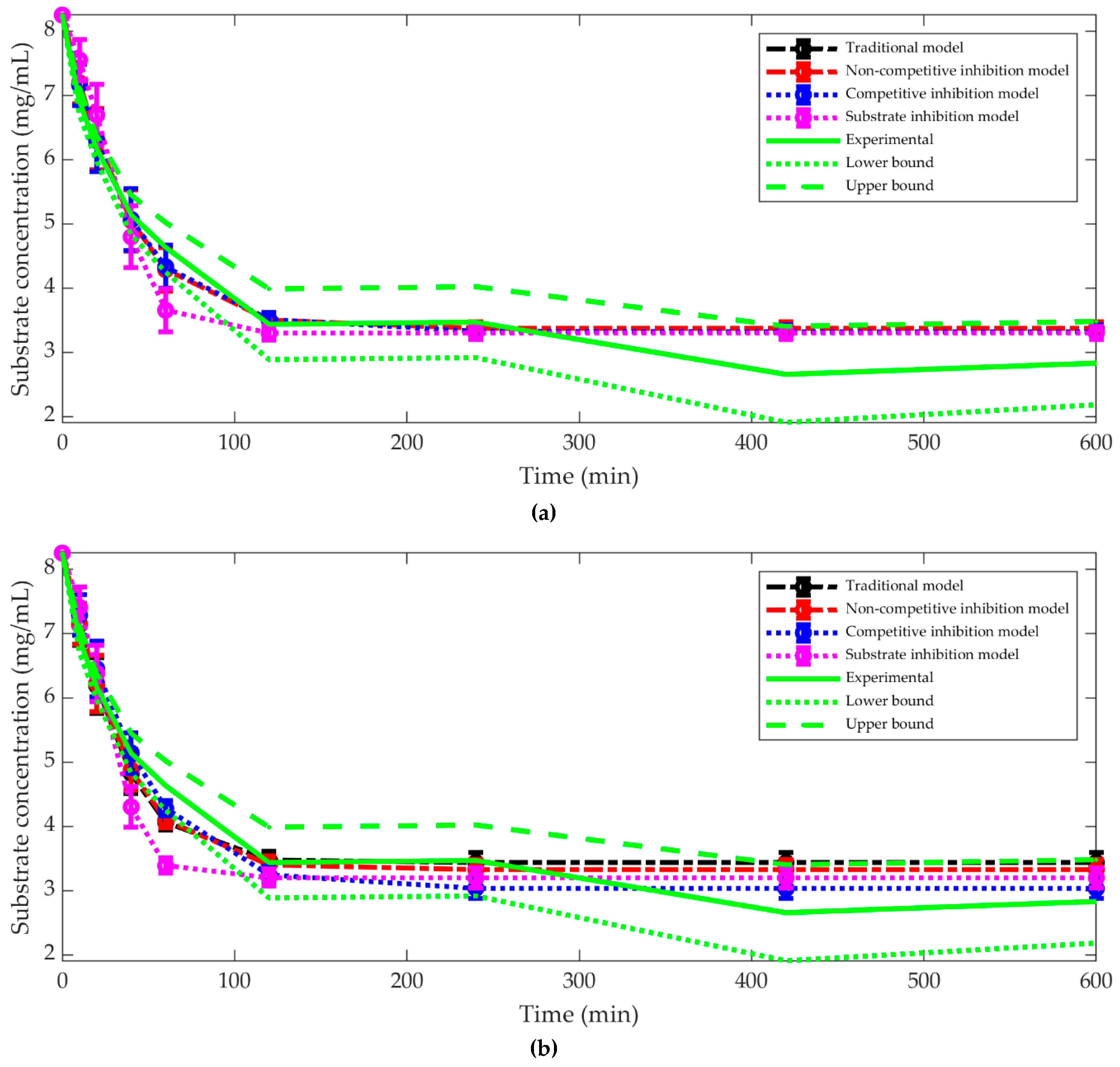
3.1. The Best Kinetic Model

Table 2 shows the best kinetic model found by each optimizer and its corresponding optimal parameter values θ * = ( V m a x * ,   K M * ,   I * ,   K * ) . It also presents the average and standard deviation of the quality measures R2, AIC, χ 2 , and MSE. As can be observed from Table 2, the least complex and best-fitting kinetic model was the Michaelis–Menten Traditional model for most of the experiments.
For the optimizers, the UMDA presented the worst performance in terms of both error and quality measures. In addition to its bad performance, the UMDA showed premature convergence on different runs. The quality measure of the UMDA was insignificantly improved as the number of iterations and the population size increased. Because of this behavior, we concluded that the UMDA is easily trapped in local minima; consequently, we hypothesize that the quality measure χ 2 is not convex.
Surprisingly, the Interior-Point algorithm dominated in determining the best-fitting model for most of the experiments. Furthermore, the MSEs in training and testing were similar. However, as can be observed in the results of Experiments 08 and 11 (Table 2), different parameter sets lead to the same quality measures. From this result, it can be concluded that χ 2 is a non-injective function of θ . Despite this result, the Interior-Point algorithm was robust enough to carry out the optimization process. The good results of the PSO in conjunction with the bad performance of the UMDA provide evidence that the quality measure χ 2 is not smooth but presents a certain degree of roughness. Therefore, optimizers that can avoid local minima like the PSO or the Interior-Point should be preferred.
Experiments 04 and 06 are two representative cases of the numerical results reported in Table 2. Figure 1 illustrates a scenario where the Nelder–Mead, PSO, and Interior-Point optimizers achieve similarly high performance, while the UMDA leads to an unsatisfactory fit, and Nelder–Mead leaves the feasible regions in the parameter search space. Figure 2 depicts one example of the two cases (Experiments 06 and 07) with the lowest performance. The graphical comparisons for the rest of the experiments are provided at the Supplementary Materials section.

3.2. Computation Time for Kinetic Parameter Optimization

A comparison of the computation time required for each optimizer to find the best kinetic parameters is depicted in Figure 3. Here, the computation time not only depends on the optimizer but also on the kinetic model being optimized. For the first three models (Michaelis–Menten, Non-competitive inhibition, and competitive inhibition), the UMDA and PSO required between 10 and 100 times the average amount of time required by the Nelder–Mead and Interior-Point algorithms to converge to their best solutions. Notably, for the Substrate Inhibition model, the UMDA and PSO (and sometimes the Nelder–Mead) optimizers presented convergence problems. These three algorithms required around 100–1000 times the amount of time compared to the time required by the Interior-Point method to converge. These problems could be due to two reasons: (i) All methods except for the Interior-Point are completely stochastic; thus, some of the random candidate solutions can be stuck in valleys of the response surface, thereby hindering the convergence of the optimizer; (ii) The Interior-Point was provided with an initial candidate solution that favors its convergence.
The optimizers were run on a computer with an Intel® (Intel Corporation, Santa Clara, CA, USA) Core™ i7 CPU @ 2.60 GHz processor, 16GB RAM, and a 256 GB hard disk. The total computation times to calibrate the first three models with the available experimental data were 0.19, 1.05, 13.06, and 33.37 min for the Nelder–Mead, Interior-Point, PSO, and UMDA algorithms, respectively. For the Substrate Inhibition model, the total computation time was 0.13, 27.54, 592.41, and 832.15 min for the Interior-Point, Nelder–Mead, UMDA, and PSO, respectively. In conclusion, the Interior-Point algorithm is the fastest method among the four optimizers analyzed in this work for kinetic parameter optimization. Nelder–Mead is also fast, but it is not recommended because it converges to unfeasible regions and is sensitive (like the UMDA and PSO) to the typical randomized initialization of metaheuristics for complex models such as Substrate Inhibition.

3.3. Comparison between Micro-Reaction and Bench Scale Reactor

As a final experiment, the values of the kinetic parameters for the optimized experiment in the micro-reaction were obtained. The values of the parameters Vmax, Km, and K were 1.06 mg/Ml × s, 8.24 mg/mL, and 0.27, respectively. The data were obtained using the IPA method and the traditional kinetic model according to the conclusions derived from Table 2. Figure 4 depicts the trajectory of the optimized micro-reactor compared to the three bench scale reactors. According to the results presented in [12], a micro-scale experiment was developed using the optimal parameters obtained by the central composite design, and these parameters were also used to test the experiment on a scale of 0.5 L.
Notably, the difference in size between the two reported experiments is 500 times higher. Furthermore, the reported micro-scale experiments were tested by orbital shaking at a speed of 700 rpm and a very stable temperature control with variations of ±1 °C. The difference with the 0.5 L reactor was the use of propeller agitation (150 rpm), ensuring that all the reactor contents were well mixed to ensure spatial homogeneity. Further studies should be done to ensure spatial homogeneity, but this goal is beyond the scope of this work.
According to the results, the Traditional model with its optimized parameters was able to predict the behavior in the micro-reaction, showing R 2 = 0.99 and M S E = 0.06 . In addition, the same model and parameters predicted the behavior of the reaction on a bench scale for three different reactors, achieving performance of ( R 2 = 0.96 ; M S E = 0.30 ) , ( R 2 = 0.93 ;   M S E = 0.54 ) , and ( R 2 = 0.97 ; M S E = 0.22 ) for reactors 1, 2, and 3, respectively. Therefore, the behavior of depolymerization on a bench scale can be predicted with acceptable errors using micro-reaction experiments.

4. Discussion

The results in Table 2 present the best-fit model found by each optimizer. To clarify the differences between the best-fitted model and the rest of the models, Figure 5 provides a graphical comparison of the four M–M models calibrated using the four optimization strategies for Experiment No. 13. Figure 5a–c depict the fit obtained by both IPA and PSO, which reached the same R2 of 0.93, but the AIC value for the IPA method was lower (−3.06). Consequently, we observed a better fit in Figure 5a than in Figure 5b. The UMDA optimizer, shown in Figure 5c, presents an R2 of 0.86 and an AIC of 1.02. UMDA presents a poor fit compared to the three previous methods, but it also adequately recapitulates the trajectory shown by the experimental data.
The parameters Vmax and KM characterize the enzymatic reactions that are described with the kinetics of M–M. Vmax depends on the total concentration of the enzyme, but KM does not [14]. KM is equal to the concentration of the substrate at half Vmax. It can also be associated with the affinity of the enzyme for the substrate [3]. As reported by Cho et al. [3], a low KM value indicates a sizeable binding affinity, as the reaction approaches Vmax more rapidly. Furthermore, a high KM indicates that the enzyme does not bind as efficiently with the substrate, and Vmax will only be reached if the substrate concentration is high enough to saturate the enzyme [3]. The V m a x and K m parameters were searched in (0, 8.25) and (0, 8.25), respectively. Parameter I (the inhibitor) was calculated using a range between 0 and 8.25. This range was employed because it is well known that there is an intermediate product called cellobiose during the production of glucose that exerts an inhibitory effect over biomass depolymerization reactions [2]. The maximum amount of glucose that can be ideally produced is 8.25 mg.
As previously explained, Table 2 shows the results obtained for the parameters Vmax, KM, I, K, χ 2 , and R2, as well as the error value. To explain the kinetic parameters (Vmax and KM), Experiment 11 and 12 were used (Figure 6). Experiments 11 and 12 have the same characteristics with the exception of temperature: Experiment 11 @ pH = 5; T = 65 °C; enzyme–substrate ratio = 0.9 µL of enzyme/g of substrate; Experiment 12 @ pH = 5; T = 45 °C; enzyme–substrate ratio = 0.9 µL of enzyme/g of substrate. The Vmax and KM values for Experiment 11 were 3.83 mg/mL·s and 7.26 mg/mL, indicating that the Vmax was quickly reached due to the affinity of the enzyme with the substrate, probably associated with the effect of the temperature. It is well known that a high temperature favors enzymatic reactions. The results agree with the low KM value obtained, which is associated with a high affinity between the enzyme and the substrate.
On the other hand, Experiment 12 shows a low Vmax (0.19 mg/mL·s) and a high KM value (8.25 mg/mL). The high KM value indicates that the enzyme–substrate affinity is low; however, it allows the experiment to attain a higher depolymerization value. Both experiments show a high inhibitor value, indicating that the reaction is being inhibited. This result could be associated with a high accumulation of cellobiose during the reaction favored by temperature [2]. A graphic compilation of all the methods obtained is shown in the complementary information.

5. Conclusions

For the metaheuristic optimizers, we conclude that the Interior-Point algorithm is effective for solving the inverse modeling problem of kinetic parameters for the depolymerization of biomass. If a priori information, such as the initial candidate solution, is available, the Interior-Point should be the first option; if not, the PSO may be considered. The default values were shown to be sufficient for all the optimizers to provide acceptable solutions. However, pure metaheuristic algorithms (like the UMDA and PSO) might further improve convergence efficiency by tuning their hyper-parameters.
The quality measure employed to evaluate the best-fitting kinetic model is likely non-convex and rough. Although many other quality measures could be used, the Weighted Least Squares metric χ 2 was enough to guide the optimizer exploration and correctly identify the best model for experimental data, at both the micro and macro scale.
The methodology applied in this study can be adopted as a starting point for solving forthcoming inverse modeling problems. The use of different metaheuristic and hybrid optimizers can reveal the nature of the quality measures, thereby easing the implicit optimization problems.
In this study, we found an effective computational procedure to determine a better calibration for mathematical models of kinetic polymerization process. However, new experiments should be considered in the future to study micro-reactions, compare these with larger scales and test multiple operating parameters. In addition, important considerations such as heat and mass transfer should be studied but are beyond the scope of this investigation.
Finally, according to our observations, the models with the best fit are not necessarily consistent with a fixed set of kinetic parameters, KM and Vmax. Therefore, to inform the best decision for the process it is necessary to discern which KM and Vmax values best describe the behavior of the evaluated reaction.

Supplementary Materials

The following are available online at https://www.mdpi.com/2227-9717/8/7/836/s1. Figure S1: Experiment 1, Figure S2: Experiment 2, Figure S3: Experiment 3, Figure S4: Experiment 4, Figure S5: Experiment 5, Figure S6: Experiment 6, Figure S7: Experiment 7, Figure S8: Experiment 8, Figure S9: Experiment 9, Figure S10: Experiment 10, Figure S11: Experiment 11, Figure S12: Experiment 12, Figure S13: Experiment 13, and Figure S14: Experiment 14.

Author Contributions

Conceptualization, C.E.M.-G. and L.C.P.; methodology, D.A.-P.; L.C.P.; software, D.A.-P.; validation, L.C.P., C.E.M.-G., E.V.-N., D.A.-P., and S.F.-G.; formal analysis, D.A.-P., L.C.P.; investigation, D.A.-P., S.F.-G., L.C.P., E.V.-N., C.E.M.-G.; resources, D.A.-P., S.F.-G.; writing—original draft preparation, L.C.P.; D.A.-P.; C.E.M.-G.; writing—review and editing, E.V.-N.; S.F.-G.; C.E.M.-G.; funding acquisition, L.C.P. and S.F.-G. All authors have read and agreed to the published version of the manuscript.

Funding

This research was funded by “PRODEP-SEP grant number 511-6/17-8432” and “The Secretaría de Innovación, Ciencia y Educación Superior grant number SICES; IJ-19-36”.

Acknowledgments

E Vázquez-Núñez gives thanks to the University of Guanajuato for all the facilities and to B VF for her patient support, CE Molina-Guerrero acknowledges the Division of Sciences and Engineering of the University of Guanajuato, Campus León, for the support of this project.

Conflicts of Interest

The authors declare no conflict of interest.

References

  1. Molina-Guerrero, C.E.; de la Rosa, G.; Castillo-Michel, H.; Sánchez, A.; García-Castañeda, C.; Hernández-Rayas, A.; Valdez-Vazquez, I.; Suarez-Vázquez, S. Physicochemical Characterization of Wheat Straw during a Continuous Pretreatment Process. Chem. Eng. Technol. 2018, 41, 1350. [Google Scholar] [CrossRef]
  2. Sakimoto, K.; Kanna, M.; Matsumura, Y. Kinetic model of cellulose degradation using simultaneous saccharification and fermentation. Biomass. Bioenergy 2017, 99, 116–121. [Google Scholar] [CrossRef]
  3. Cho, Y.S.; Lim, H.S. Comparison of various estimation methods for the parameters of Michaelis–Menten equation based on in vitro elimination kinetic simulation data. Transl. Clin. Pharmacol. 2018, 26, 39–47. [Google Scholar] [CrossRef] [PubMed] [Green Version]
  4. Valencia, P.; Cornejo, I.; Almonacid, S.; Teixeira, A.A.; Simpson, R. Kinetic Parameter Determination for Enzyme Hydrolysis of Fish Protein Residue Using D-optimal Design. Food Bioprocess. Tech. 2013, 6, 290–296. [Google Scholar] [CrossRef]
  5. Pernice, S.; Follia, L.; Balbo, G.; Milanesi, L.; Sartini, G.; Totis, N.; Lió, P.; Merelli, I.; Cordero, F.; Beccuti, M. Integrating Petri Nets and Flux Balance Methods in Computational Biology Models: A Methodological and Computational Practice. Fundamenta Informaticae 2019, 171, 367–392. [Google Scholar]
  6. Chou, I.C.; Voit, E.O. Recent developments in parameter estimation and structure identification of biochemical and genomic systems. Math. Biosci. 2009, 219, 57–83. [Google Scholar] [CrossRef] [PubMed] [Green Version]
  7. Kruse, R.; Borgelt, C.; Braune, C.; Mostaghim, S.; Steinbrecher, M. Introduction to computational intelligence. In Computational Intelligence; Springer: London, UK, 2014; Volume 62, pp. 3–17. ISBN 9781447172963. [Google Scholar]
  8. Quaranta, G.; Lacarbonara, W.; Masri, S.F. A Review on Computational Intelligence for Identification of Nonlinear Dynamical Systems; Springer: Amsterdam, The Netherlands, 2020; Volume 99, ISBN 1107101905. [Google Scholar]
  9. Tangherloni, A.; Spolaor, S.; Cazzaniga, P.; Besozzi, D.; Rundo, L.; Mauri, G.; Nobile, M.S. Biochemical parameter estimation vs. benchmark functions: A comparative study of optimization performance and representation design. Appl. Soft Comput. 2019, 81, 105494. [Google Scholar] [CrossRef]
  10. Rojas-Dominguez, A.; Padierna, L.C.; Carpio Valadez, J.M.; Puga-Soberanes, H.J.; Fraire, H.J. Optimal Hyper-Parameter Tuning of SVM Classifiers with Application to Medical Diagnosis. IEEE Access 2017, 6, 7164–7176. [Google Scholar] [CrossRef]
  11. Berlin, A.; Maximenko, V.; Bura, R.; Kang, K.Y.; Gilkes, N.; Saddler, J. A rapid microassay to evaluate enzymatic hydrolysis of lignocellulosic substrates. Biotechnol. Bioeng. 2006, 93, 880–886. [Google Scholar] [CrossRef] [PubMed]
  12. Molina, C.; Sánchez, A.; Serafín-Muñoz, A.; Folch-Mallol, J. Optimization of Enzymatic Saccharification of Wheat Straw in a Micro-Scale System By Response Surface Methodology. Rev. Mex. Ing. Quím. 2014, 13, 765–778. [Google Scholar]
  13. Molina Guerrero, C.E.; De la Rosa, G.; Gonzalez Castañeda, J.; Sánchez, Y.; Castillo-Michel, H.; Valdez-Vazquez, I.; Balcazar, E.; Salmerón, I. Optimization of Culture Conditions for Production of Cellulase by Stenotrophomonas maltophilia. BioResources 2018, 13, 8358–8372. [Google Scholar] [CrossRef]
  14. Fogler, S. Elements of Chemical Reaction Enginnering, 5th ed.; Prentice Hall: Upper Saddle River, NJ, USA, 2020. [Google Scholar]
  15. Strutz, T. Data Ftitting and Uncertainity, 1st ed.; Springer Fachmedien: Heidelberg, Germany, 2011; ISBN 9783834810229. [Google Scholar]
  16. Talbi, E.-G. Metaheuristics: From Design to Implementation, 1st ed.; John Wiley & Sons, Inc.: Hoboken, NJ, USA, 2009; ISBN 9780470278581. [Google Scholar]
  17. Aztatzi-Pluma, D.; Figueroa-Gerstenmaier, S.; Padierna, L.C.; Vazquez-Nuñez, E.; Molina-Guerrero, C.E. Análisis paramétrico de la depolimerización de paja de trigo en un sistema en microescala. In Proceedings of the XLI Encuentro Nacional de la AMIDIQ, Ixtapa, Mexico, 27–30 October 2020. (In Spanish). [Google Scholar]
  18. Larrañaga, P. A Review on Estimation of Distribution Algorithms. In Estimation of Distribution Algorithms, 1st ed.; Springer: Boston, MA, USA, 2002. [Google Scholar]
  19. Kennedy, J.; Eberhart, R. Particle Swarm Optimization. In Proceedings of the Proceedings of ICNN’95—International Conference on Neural Networks, Perth, WA, Australia, 27 November–1 December 1995; pp. 1942–1948. [Google Scholar]
  20. Byrd, R.; Hribar, M.; Nocedal, J. An Interior Point Algorithm for large-scale Nonlinear Programming. Ind. Eng. Manag. Sci. 1999, 9, 877–900. [Google Scholar] [CrossRef]
  21. Hauschild, M.; Pelikan, M. An introduction and survey of estimation of distribution algorithms. Swarm. Evol. Comput. 2011, 1, 111–128. [Google Scholar] [CrossRef] [Green Version]
  22. Zhang, Q.; Mühlenbein, H. On the Convergence of a Class of Estimation of Distribution Algorithms. IEEE T. Evolut. Comput. 2004, 8, 127–136. [Google Scholar] [CrossRef]
  23. Poli, R.; Kennedy, J.; Blackwell, T. Particle swarm optimization: An overview. Swarm. Intell. 2007, 1, 33–57. [Google Scholar] [CrossRef]
  24. Rao, S.S.; Mulkay, E. Using Interior-Point Algorithms. AIAA J. 2000, 38, 2127–2132. [Google Scholar] [CrossRef]
  25. Vanderbei, R. Linear Programming: Foundations and Extensions, 5th ed.; Springer: New York, NY, USA, 2020; ISBN 9783030394141. [Google Scholar]
  26. Lustig, I.J.; Marsten, R.E.; Shanno, D.F. Feature Article—Interior Point Methods for Linear Programming: Computational State of the Art. ORSA J. Comput. Publ. 1994, 6, 1–14. [Google Scholar] [CrossRef] [Green Version]
  27. Hofstee, B.H.J. On the Evaluation of the Constants Vm and KM in Enzyme Reactions. Science 1952, 116, 329–331. [Google Scholar] [CrossRef]
  28. Murphy, A. The Coefficients of Correlation and Determination as Measures of Performance in Forecast Verification. Weather Forecast. 1995, 10, 681–688. [Google Scholar] [CrossRef] [Green Version]
  29. Dutta, K.; Dasu, V.V.; Mahanty, B.; Prabhu, A.A. Substrate Inhibition Growth Kinetics for Cutinase Producing Pseudomonas Substrate Inhibition. Chem. Biochem. Eng. Q. 2015, 3, 437–445. [Google Scholar] [CrossRef]
Figure 1. Best-fit models for data in Experiment No. 4 (pH = 5.7, T = 48 °C, enzyme–substrate ratio = 0.3343 μ L enzyme/g cellulose). Interior-Point and particle swarm optimization (PSO) accurately fitted the experimental data ( R 2 = 0.98 . Mean square error (MSE) = 0.7), while the Univariate Marginal Distribution algorithm (UMDA) presents larger errors ( R 2 = 0.86 . M S E = 0.57 ). The standard deviations reported in Table 2 should be carefully interpreted. For instance, the case of PSO with a mean value of R 2 = 0.8 and standard deviation of 0.33 were the result of evaluating the model with four training data folds, which reached R 2 values of 0.95, 0.30, 0.96, and 0.98, respectively.
Processes 08 00836 g001
Figure 2. Best-fit to experimental data for Experiment No. 6 (pH = 5.7, T = 62 °C, enzyme–substrate ratio = 0.3343 μ L enzyme/g cellulose). The kinetic parameter found by the four optimizers lead to the lowest calibration to experimental data.
Processes 08 00836 g002
Figure 3. Comparison of the computation time required by each optimizer to find the best kinetic parameters. According to the difficulty of being optimized, the kinetic models are grouped into two categories, i.e., the first group with three models: (a) Michaelis–Menten, (b) non-competitive inhibition and (c) competitive inhibition, and the second group with (d) the Substrate Inhibition model.
Processes 08 00836 g003
Figure 4. Comparison between micro-reaction and bench scale reactor trajectory assayed with the same operational parameters (pH 4.64; T 52 °C; enzyme–substrate ratio = 1.8 mL enzyme/g cellulose).
Processes 08 00836 g004
Figure 5. Graphical comparison of the four M–M models calibrated by four optimization strategies: (a) Interior-Point Algorithm; (b) Particle Swarm Optimization and (c) Univariate Marginal Distribution Algorithm. Experiment 13 at pH = 5; T = 55 °C; enzyme–substrate ratio = 1.8 µL of enzyme/g of substrate.
Processes 08 00836 g005aProcesses 08 00836 g005b
Figure 6. Comparison of the four M–M models calibrated by Interior-Point strategy; (a) and (b) Experiment 11 @ pH = 5; T = 65 °C; enzyme–substrate ratio = 0.9 µL of enzyme/g of substrate; (c) and (d) Experiment 12 @ pH = 5; T = 45 °C; enzyme–substrate ratio = 0.9 µL of enzyme/g of substrate.
Processes 08 00836 g006
Table 1. Experimental conditions for enzyme depolymerization at micro-scale. pH stands for potential of hydrogen.
ExperimentpH°CµL/mgExperimentpH°CµL/mg
14.3481.465684.0550.9000
24.3620.334396.0550.9000
34.3621.4656105.0450.9000
45.7480.3343115.0650.9000
55.7481.4656125.0550.1000
65.7620.3343135.0551.8000
75.7621.4656145.0550.9000
Table 2. Best-fitting models and parameters found by optimizer: Interior-Point Algorithm (IPA), Particle Swarm Optimization (PSO) and Univariate Marginal Distribution Algorithm (UMDA). Vmax (mg/mL × s), KM (mg/mL), I (mg/mL). MSE: mean square error.
ExperimentOptimizerBest-Fitting Kinetic ModelR2 TrainAIC Mean ± Std χ 2 VMax*Km*K* I * MSE TrainMSE Test
1IPATraditional0.98 ± 0.03−15.29 ± 11.522.77 ± 5.01.430.581.25 0.02 ± 0.030.01 ± 0.02
PSOTraditional0.88 ± 0.10−2.01 ± 5.8015.76 ± 3.590.838.250.32 0.19 ± 0.191.05 ± 1.38
UMDANon-Competitive I.0.81 ± 0.122.88 ± 5.1123.55 ± 14.62.193.290.804.330.31 ± 0.230.76 ± 0.57
2IPATraditional0.86 ± 0.21−11.08 ± 5.4512.72 ± 19.331.058.250.44 0.06 ± 0.060.08 ± 0.07
PSONon-Competitive I.0.82 ± 0.25−8.92 ± 6.3231.17 ± 55.713.218.250.734.020.06 ± 0.050.09 ± 0.06
UMDANon-Competitive I.0.82 ± 0.14−6.33 ± 5.8116.19 ± 19.773.474.211.046.660.09 ± 0.070.1 ± 0.09
3IPATraditional0.90 ± 0.16−4.63 ± 8.436.32 ± 8.780.558.250.17 0.17 ± 0.220.39 ± 0.02
PSOCompetitive I.0.90 ± 0.14−2.51 ± 6.857.3 ± 9.951.157.840.158.110.16 ± 0.150.18 ± 0.11
UMDASubstrate I.0.81 ± 0.101.63 ± 4.0622.12 ± 14.814.967.741.23 0.39 ± 0.170.81 ± 0.63
4IPATraditional0.98 ± 0.01−7.79 ± 3.6643.98 ± 58.020.178.250.04 0.07 ± 0.050.73 ± 1.14
PSONon-Competitive I.0.80 ± 0.336.67 ± 9.17144.2 ± 188.178.040.102.628.250.57 ± 0.870.85 ± 1.25
UMDASubstrate I.0.86 ± 0.073.73 ± 3.13227.62 ± 121.34.806.401.26 0.49 ± 0.211.12 ± 0.91
5IPANon-Competitive I.0.87 ± 0.063.97 ± 2.137.01 ± 65.490.388.250.120.0010.37 ± 0.130.65 ± 0.62
PSONon-Competitive I.0.84 ± 0.085.06 ± 2.5537.19 ± 65.922.162.310.67.970.44 ± 0.201.03 ± 1.01
UMDANon-Competitive I.0.78 ± 0.146.48 ± 1.8538.14 ± 66.291.525.780.347.940.56 ± 0.160.75 ± 0.60
6IPANon-Competitive I.0.72 ± 0.15−20.73 ± 6.9812.86 ± 4.662.068.250.995.580.01 ± 0.010.01 ± 0.00
PSOTraditional0.81 ± 0.09−20.64 ± 4.588.89 ± 3.075.370.664.90 0.01 ± 0.010.01 ± 0.01
UMDATraditional0.64 ± 0.04−21.18 ± 1.9915.48 ± 1.566.366.353.50 0.01 ± 0.000.02 ± 0.01
7IPACompetitive I.0.76 ± 0.33−22.2 ± 3.8747.33 ± 83.022.131.501.445.580.01 ± 0.000.02 ± 0.01
PSOTraditional0.77 ± 0.16−22.35 ± 2.6850.41 ± 78.263.818.251.80 0.01 ± 0.000.02 ± 0.02
UMDANon-Competitive I.0.82 ± 0.17−23.27 ± 3.4948.61 ± 78.276.125.152.065.220.01 ± 0.000.02 ± 0.01
8IPATraditional0.89 ± 0.16−8.22 ± 6.91396.46 ± 784.320.978.250.38 0.09 ± 0.110.06 ± 0.05
PSOTraditional0.89 ± 0.14−7.5 ± 6.02398.22 ± 782.660.883.820.5 0.10 ± 0.100.10 ± 0.07
UMDANon-Competitive I.0.75 ± 0.121.12 ± 1.54428.95 ± 764.322.573.611.400.970.27 ± 0.070.38 ± 0.71
9IPATraditional0.87 ± 0.15−6.75 ± 4.9237.31 ± 444.350.588.250.22 0.11 ± 0.100.25 ± 0.36
PSONon-Competitive I.0.86 ± 0.12−3.38 ± 2.71243.96 ± 441.487.210.186.860.00010.14 ± 0.070.11 ± 0.12
UMDANon-Competitive I.0.8 ± 0.09−0.3 ± 3.58259.85 ± 419.394.584.531.307.010.22 ± 0.100.23 ± 0.13
10IPATraditional0.88 ± 0.2−9.58 ± 6.2957.97 ± 83.540.838.250.33 0.07 ± 0.090.08 ± 0.03
PSOCompetitive I.0.9 ± 0.07−7.79 ± 6.2788.4 ± 132.631.282.470.850.230.07 ± 0.050.11 ± 0.08
UMDANon-Competitive I.0.86 ± 0.06−3.85 ± 5.2891.28 ± 70.495.054.261.397.600.13 ± 0.090.13 ± 0.13
11IPATraditional0.86 ± 0.24−18.82 ± 7.157.15 ± 102.383.837.261.83 0.01 ± 0.000.07 ± 0.09
PSOTraditional0.86 ± 0.23−16.58 ± 2.9163.04 ± 103.313.928.201.78 0.01 ± 0.000.01 ± 0.00
UMDATraditional0.86 ± 0.22−16.31 ± 2.6462.35 ± 98.775.325.063.04 0.01 ± 0.000.02 ± 0.01
12IPATraditional0.89 ± 0.071.44 ± 7.8928.75 ± 27.830.198.250.05 0.38 ± 0.240.73 ± 0.51
PSOSubstrate I.0.87 ± 0.082.5 ± 3.7768.16 ± 41.920.538.250.09 0.43 ± 0.221.09 ± 1.02
UMDASubstrate I.0.76 ± 0.185.99 ± 2.27104.04 ± 69.115.158.211.27 0.76 ± 0.280.75 ± 0.29
13IPATraditional0.93 ± 0.07−3.06 ± 6.1915.03 ± 23.470.558.250.16 0.20 ± 0.190.24 ± 0.15
PSOCompetitive I.0.93 ± 0.1−1.24 ± 6.8915.11 ± 25.020.423.990.141.910.19 ± 0.230.14 ± 0.08
UMDASubstrate I.0.86 ± 0.131.02 ± 4.8729.65 ± 35.813.647.610.84 0.35 ± 0.230.73 ± 0.70
14IPATraditional0.95 ± 0.02−7.72 ± 1.46164.65 ± 309.480.788.250.24 0.10 ± 0.030.15 ± 0.10
PSOTraditional0.85 ± 0.19−4.17 ± 4.47138.93 ± 249.871.077.150.38 0.17 ± 0.090.18 ± 0.11
UMDANon-Competitive I.0.81 ± 0.23−0.38 ± 2.95144.33 ± 247.43.942.831.146.800.22 ± 0.080.26 ± 0.23

