1. Introduction
Solid biomass combustion plants—from kilowatt-sized furnaces for domestic heating to combined heat and power plants in the megawatt range—suffer from a decisive drawback in comparison to many other (mainly fossil) alternatives due to the low quality and the challenging properties of the utilized feedstock. Inappropriate fuel quality drastically affects a biomass furnace’s behavior: Subpar biomass reduces the lifespan of a furnace and leads to operational challenges, such as corrosion, ash deposition [
1,
2,
3,
4,
5] as well as increased gaseous and particulate emissions [
6]. The majority of industrial solid biomass combustion plants rely on woody biomass (commonly known as wood chips) as feedstock. In general, wood chips and their properties are well regulated and subject to standards, such as ISO 17225 (replacing the outdated European Standard EN 14961-4 and the still wide-spread Austrian ÖNORM M7133 used among European plant operators) which defines distinct fuel quality classes based on several parameters, such as particle size distributions, moisture and ash content [
7]. These norms are often used for definitions, agreements and contract management along the wood chip supply chain. However, in the biomass plant operator’s daily practice, even the defined limits (e.g., regarding fine particle content or ash content) are regularly breached and/or not controlled. Biomass boilers running on wood chips are thus challenged by different feedstock qualities due to a multitude of different suppliers and fluctuations between individual batches. Furthermore, economic needs often act as an important driving force towards cheaper biomass resources, such as residual or waste wood, shrubs, bark or alternatives, such as straw or short rotation crops. As a consequence, operators often use mixtures of “high” and “low” quality feedstock [
8,
9]. Finally, there are also seasonal fluctuations in the moisture content, which may vary between 20 and 45 weight-% from summer to winter.
All these variations constitute a major difference between biomass furnaces and plants running on coal. The latter are typically tailored or at least adapted to a certain narrow range of fuel qualities and properties. Thus, the variety of potential operational points is by far higher in biomass combustion. Many operators use empiric/experience-based parameters, such as estimated (or guessed) moisture or fine particle contents, as input parameters for the process control system and hope for stable operation. Yet, most of the time, biomass plants react to changes in feedstock quality after the operator observes a change in measured values in their control system.
This highlights the demand for reproducible methods in order to assess fuel quality parameters prior to the combustion process itself. Such an approach would be possible to proactively control and adapt a biomass furnace to future conditions. As a result, this mitigates the risk or the amount of slag and ash deposits and enhances the plant’s performance both in efficiencies and economic parameters.
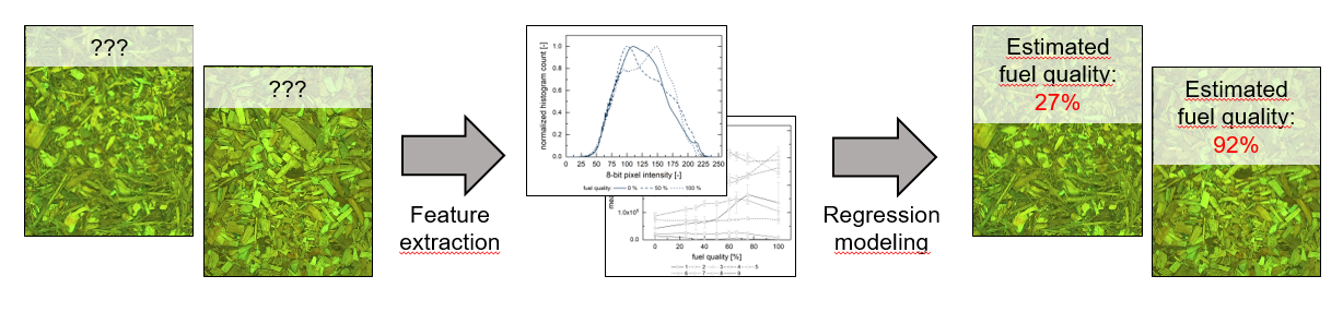
A promising method for the pre-evaluation of biomass feedstock is optical analysis (in the most basic case, image capturing through photography) followed by image evaluation. Such a technology is capable of running continuously without any need for human intervention or interaction (e.g., by observing fuel conveyor belts, stokers or chain conveyors). Moreover, it is a non-intrusive measurement method which can be easily retrofitted into the fuel feeding systems of biomass plants. This potentially enables an a priori determination of feedstock properties.
The contact-free analysis of biomass feedstock has been a subject of more and more interest over recent years. Back in 2001, Swedish researchers stated that continuous image analysis in order to characterize biomass fuels was too time consuming and “tedious” [
10]. However, due to the increase in computational resources and novel technology, this has changed drastically. The literature shows a variety of image evaluation techniques for multiple purposes and applications. The authors in [
11] give a good overview on the optical analysis of particle properties; however, they focus on individual particles instead of those in bulk. Rezaei et al. examine single wood particles with microscopes and scanners in [
12], focusing on particle properties after a grinding/milling process. Igathinathane et al. present a methodology in order to understand, improve and potentially replace the sieving of biomass particles via computer vision in [
13]. The authors state that image analysis potentially hurdles the drawbacks of sieving irregularly shaped particles, such as fibers. In [
14], Ding et al. describe an approach in order to characterize wood chips (as a resource for paper production) from images using artificial neural networks and regression models based on color features, size determination by means of granulometry and near infrared (NIR) sensors for moisture detection. Since then, NIR became a commonly used technique, especially for online moisture measurements [
15,
16,
17,
18,
19]. These approaches are often combined with regression modeling or artificial neural networks/deep learning approaches. Tao et al. [
20], for instance, describe a methodology based on IR spectra and regression modelling in order to characterize fuels regarding their chemical constituents and heating value. In [
21,
22,
23], the authors aim at determining biomass heating values by means of artificial neural networks, support vector machines and random forest models, based on measured particle properties as input parameters. Machine learning models can further be used in order to tackle and forecast the operational problems of biomass furnaces, identifying stable and beneficial operational points [
24].
Ongoing research at FAU aims at the development of an online fuel quality estimator, based on images of raw feedstock prior to the combustion process. The system targets industrial combustion plants of all sizes up to the megawatt range. In order to address small-scale (i.e., in the 100 kW range) furnaces as well, we based our methodology on consumer-grade hardware.
This study aims to examine the viability of an image-based assessment of mixing ratios of two distinct varieties of woody biomass. Storing fuel in at least two stockpiles of feedstock labelled as “high” and “low” quality, respectively, is a common practice for biomass plant operators. As mentioned above, this allows for the mixture of different grades of feedstock in order to tailor fuel with acceptable, yet economic, parameters and properties. Our goal is to determine the mixture fraction of two fuels prior to its feeding into a combustion chamber. For this task, we used a machine learning/regression modeling approach, based on feature vectors derived from image data taken in a lab-scale environment. We discuss two different approaches for feature vector generation—one based on spatially-resolved, one relying on integral information—and several linear and non-linear regression models. The modeling results are discussed with respect to their statistical accuracies, parametrization and the training strategy. Eventually, since the approach ought to be applicable for biomass furnaces in the megawatt range, we evaluate several simplified training approaches based on few input parameters which can be applied during the ongoing operation of biomass power plants. Since the modeling accuracy suffers from these simplifications, we estimate necessary sampling sizes in order to maintain an appropriate predictive quality. This study is, therefore, a first and a major step towards the development of a proactive biomass furnace control system with respect to incoming feedstock.
2. Materials and Methods
2.1. Fuel Selection and Classification
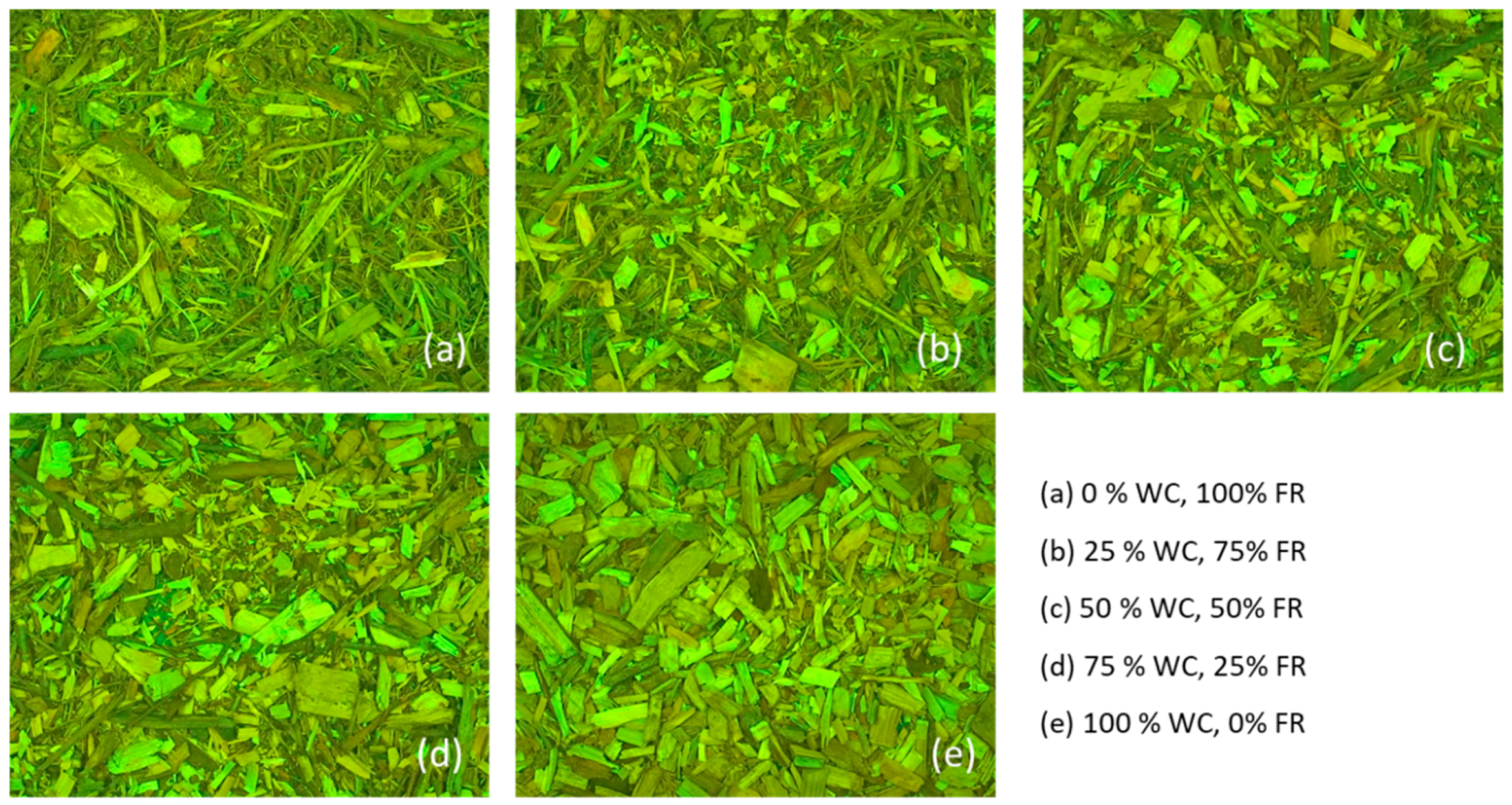
For this work, we used feedstock from the Bad Mergentheim biomass combined heat and power (CHP) plant in Southern Germany running on wood chips (WC) and forest residual wood (FR). The operator intended to run on a 50/50 mixture; however, since “mixing” happens with a bulldozer on the yard, the actual composition was subject to fluctuations. We took samples for the optical analysis from the WC and FR stockpiles in August 2019. WC principally consist of pine stem wood from the German Tauberfranken region with low shares of bark and branches. In contrast, FR is a mixture of soft and hardwood featuring a high amount of branches, leaves, needles and shrubs. Both fractions can be visually distinguished. Due to the summertime sampling and the preceding yard storage, both of the fuels exhibited low water content in the range of 18.9 ± 0.9% (WC) and 22.6 ± 1.0% (FR), based on nine measurements over the batch size. WC featured a lower ash content of 3.8 ± 1.2% compared to FR (5.9 ± 0.2%). For both fuels, a sieve analysis revealed that between 88% and 97% of the fuel mass originated from particles larger than 5 mm, and 98.8 to 99.5% of the mass from particles larger than 1 mm. A major difference between WC and FR lay in their bulk densities, which we determined according to ISO 17828. With a bulk density of 222 ± 23 kg/m
3, WC featured an approximately 75% higher value than FR (125 ± 12 kg/m
3). Measuring the bulk density of a mixture (1:1) of these fuels led to 176 ± 9 kg/m
3, a value lying close to the calculated average. The lower value of FR is not surprising, as it results from the generally higher aspect ratios and irregular shapes of individual particles, due to the high amounts of branches and bark.
Table 1 sums up the determined fuel properties.
For this study, we created a total of nine different mixtures based on distinct volumetric ratios. Volumetric ratio was chosen due to the aforementioned real-life comparison process of mixing with a bulldozer. Besides the 0/100 and 100/0 mixture classes, we prepared ratios of 25/75, 33/66, 40/60, 50/50, 60/40, 66/33 and 75/25. Thus, there was an intended higher amount of data for mixtures close to the operator’s target mixture of 50/50.
Figure 1 displays exemplary representatives from five of the fuel classes. In this article, we use the term “fuel quality” in order to address certain mixture ratios: 0% fuel quality refers to pure FR; 50% means a volumetric ratio of 1:1 (FR:WC); 100% is solely WC (i.e., the high quality feedstock).
2.2. Image Capturing
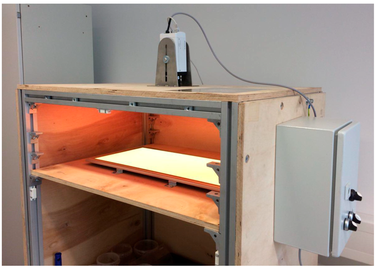
In order to capture representative fuel images, we used a closed box with two planar LED panels for artificial lighting. This ensured the absence of ambient light, thus enabling a representative image capturing process. The color of the LED could be altered; however, we observed no influence on the regression modelling results, especially since the evaluation happened on greyscale images anyway. Thus, all images were taken with green light from above as incident light. The camera was a SONY SNC-VB600B IP camera with a maximum resolution of 1280 × 1024 pixels. The decision towards a robust consumer-type camera was due to the project’s goal of implementing a similar setup into biomass-fired power plants and furnaces, and developing an economically feasible fuel analysis setup, even for small combustion plants. All of the pictures were taken through a window made of acrylic glass from a distance of 450 mm, capturing a total area of 480 × 360 mm.
Figure 2 depicts the experimental setup. Image capturing happened automatically by means of a script written in the Python programming language. For each of the presented fuel classes, we took between 32 and 40 different photographs (325 in total), shuffling the samples between each shot. In order to avoid three-dimensional mixing effects due to different particle shape, the feedstock was spread in a layer of only approximately 5 cm height.
2.3. Image Processing
2.3.1. Preprocessing
Image preprocessing started with the application of a smoothing filter by means of a bilateral filter. This operation reduced unwanted noise while maintaining sharp edges. In comparison to other smoothing filters, such as the Linear or Gaussian Blur convolution, bilateral filtering recognizes and ignores high gradients in pixel intensities—especially occurring at edges—during smoothing by combining both a similarity/intensity and a distance/coordinate kernel [
25]. Subsequently, the RGB (red, green, blue) images were transformed into 8-bit greyscale images.
2.3.2. Feature Vector Formulation
In order to successfully apply regression modelling to the image matrices, it was necessary to reduce the amount of information drastically by identifying, describing and quantifying one or several characteristic features. The so-called feature vector included the entirety of features and was used for model training.
In this case, we examined two different approaches in order to formulate feature vectors for their applicability. The first method relied on the greyscale (8-bit) histograms (i.e., representing the images’ pixel brightness distribution densities). In contrast to that, the second approach recognized the spatial distribution of the pixels by calculating textural features, known as Haralick features [
26]. After the calculation of both features, all of the data were normalized. Data standardization (i.e., dividing the data by the standard deviation after subtracting the respective mean value) was also evaluated, but it was not applied since it did not enhance the results, but rather increased the noise.
2.3.3. Histogram-Based Feature Vector
The 8-bit greyscale image potentially consisted of 28 = 256 different values, so calculating the histogram reduced the amount of information from width x height (pixels) to 256. The feature vector’s size could decrease even further by applying different techniques, such as histogram equalization (i.e., neighboring brightness values aggregated into bigger classes) or simply ignoring low-intensity histogram areas (in photographs often close to 0 or 255; i.e., pure white and dark black).
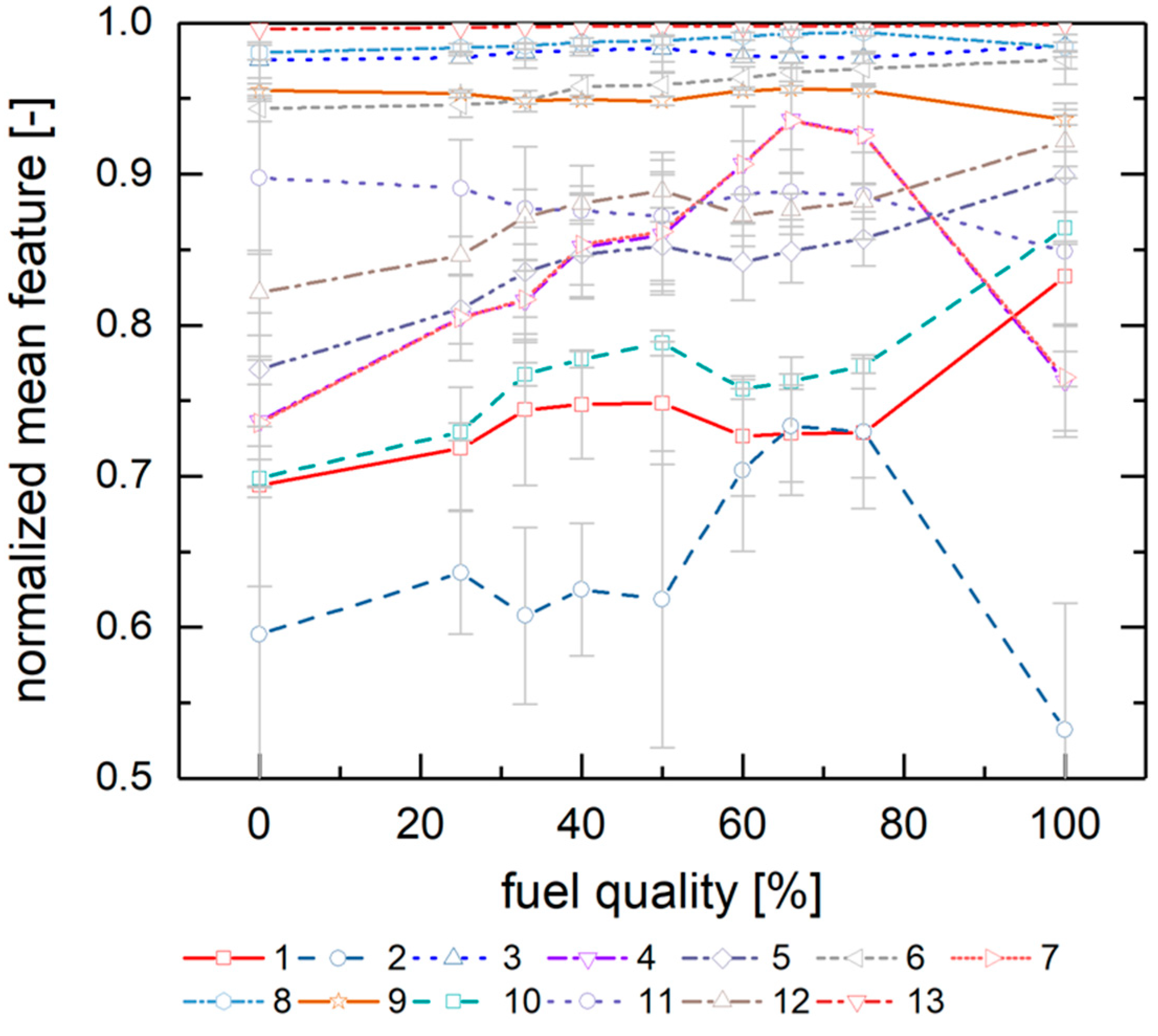
Figure 3 depicts the averaged normalized histograms of the 0, 50 and 100% fuel quality classes. The fuel images exhibit close to no pixel values in the highest and lowest value ranges, so these were neglected for the feature vector formulation. Subsequently, the histogram was reduced to nine features representing pixel values from 90 to 180 in equidistant steps (with feature 1 at 90 pixels and feature 9 at 180 pixels); these data were exported to the image’s feature vector. This approach is the result of an examination (which is not discussed in detail here) of the behavior different possible feature vectors extracted from the histogram; the chosen method leads to the most promising results.
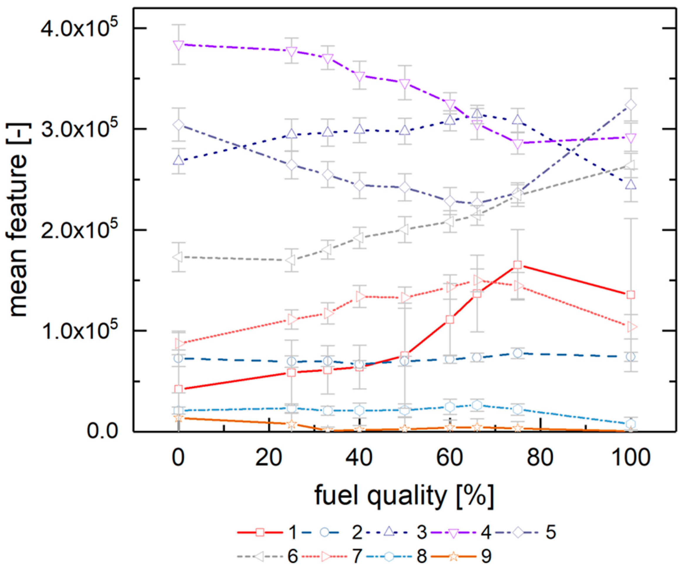
Figure 4 displays the resulting mean values for the nine fuel quality classes and their standard deviations. The latter thus indicates the typical deviations from the average values. Please note that the
y-axis contains the data (with pixel counts as unit) before normalization for reasons of better visibility. The feature vector training takes place with normalized data, though.
2.3.4. Texture-Based Feature Vector
The calculation of the Haralick texture features happened analogous to [
26], based on greyscale images and the co-occurrence matrix G:
where
Ng is the total number of an image’s grey values and
p(i,j) describes the probability that a pixel
i is located in adjacency to a pixel with a value of
j.
Haralick et al. propose a total set of 14 different features which are a measure of the spatial relationship of the pixels [
26]. Most of them are obtained by calculating the sum of characteristic information over the co-occurrence matrix
p(i,j). This includes statistical information, such as the variance, average, correlation coefficients and the sum of squares of pixel intensities, as well as moments and the image’s entropy. [
26]
We calculated the Haralick features in this work by means of its implementation in the “mahotas” Python package [
27]. For stability reasons, this module included only the first 13 Haralick features (as is a common approach in the literature [
28,
29]), which are subsequently used as feature vectors in normalized form.
Figure 5 depicts the resulting 13 normalized Haralick features for the different fuel classes, highlighting their mean values and the corresponding standard deviations.
2.4. Regression Model Selection and Setup
Although the training data fall into up to nine distinct classes, we regard the fuel mixture analysis as a regression problem instead of a task for classification. This is due to the circumstance that the real-world application will challenge the model with data which might lie in-between distinct classes. For this reason, interpolation between individual classes might become appropriate. In order to train a regression model, the data need to be subdivided into two subsets, a set used for training and model generation, and a test/holdout set in order to validate the resulting model with “unknown” data. For this work, we split the images into 80% for training and 20% for testing. To make the best use of the data set, consisting of 325 images, the 5-fold cross validation, a commonly used form of the k-fold cross validation, found application in the training process [
30].
In the course of this work, we evaluated a total of seven different regression models under varying parametrization. Although the extracted features did not behave linearly, there was no very prominent nonlinearity either. Consequently, three different linear regression models were tested [
30]:
Ordinary least squares Linear Regression
Lasso Linear Regression featuring L1 regularization
Ridge Linear Regression with L2 regularization
L1 and L2 regularizations refer to the exponent k = 1 or 2 in an additional penalty term in the loss function L, which potentially avoids overfitting (L1) or reduces the impact of irrelevant features (L2):
where
yi and
are the actual and predicted data, respectively. For
= 0, Equation (2) equals the ordinary least squares loss function. The model generally seeks to minimize
L by identifying (“learning”) appropriate coefficients
in an iterative process for the target function:
Furthermore, we applied four non-linear regression algorithms, more precisely four kinds of tree-based methods [
30]:
Decision Tree Regression (DT)
Random Forest Regression (RF)
Gradient Boosting Regression (GB) and
Extra Tree Regression (ET).
These modeling algorithms rely on the development of one or several tree-shaped structures, starting from a root node and subsequent decision nodes (“parent nodes”) of a different hierarchy from where further branches (“child nodes”) originate until the respective section terminal node. The predicted value depends on the reached final node after finding a pathway from the root to a terminal node. Tree-type models are parametrized by defining or limiting the number of layers, branches or nodes, as well as the minimum sample number needed at a certain node in order to provoke the formulation of child nodes. The DT algorithm results in a single tree, while the RF and GB models consist of a large number of combined trees (with the difference between RF and GB lying in the moment of combination). Eventually, the ET algorithm is a RF derivative that does not split at certain optimized ratios of features at a point, but randomly. This may prevent overfitting and is often computationally cheaper due to the lack of one optimization step. The RF, GB and ET algorithms lead to so-called ensemble models, since they combine a group of weak learners in order to create one model with high predictive accuracy. For this purpose, they apply the bagging and boosting techniques. The first (i.e., bagging) refers to the parallel development of a high number of different modelling manifestations; the final predictions originate from the aggregated individual predictions. Boosting, on the other hand, is the sequential training of several weak regressors, which influence and correct upstream learners.
RF and ET apply bagging as an ensemble model. GB obviously uses boosting per se; regarding the other models, we trained and evaluated several boosted models using the AdaptiveBoosting (adaboost) algorithm [
31] with the respective base estimator.
The models were used as implemented in the scikit-learn Python programming language module [
32].
2.4.1. Model Evaluation and Error Estimation
The evaluation of the models’ performances relied on metrics commonly used in statistical analysis (cf. Kuhn and Johnson [
30]). For the following mathematical representations, the data set n consisted of true or observed values y
i and its corresponding prediction or modelled value
of the
ith sample
.
In order to assess the predictive quality, we used the coefficient of determination
R2:
R2 is the squared correlation coefficient, yielding information about the amount of data points being well represented by the model; R2 is consequently highly affected by outliers. Since the model training happens with 5-fold cross validation, the accuracy can be denoted as a mean value of R2 and its standard deviation.
The mean squared error (MSE) and root mean squared error (RMSE) both indicate the scattering of predicted values around the real value. Since the dimension of RMSE is similar to the evaluated data, it is easy to assess and a quite intuitive parameter:
Besides the irreducible error (noise), MSE includes both the model’s bias and variance:
Low MSE values thus indicate some scattering and a lower risk of unwanted overfitting. Generally, there is a trade-off between bias and variance, which makes it impossible to minimize both parameters. The method of bias–variance decomposition can be used in order to evaluate the contribution of variance and bias by solving a quadratic equation, including the expected error
E:
2.4.2. Parameter Variations
In order to identify the most suitable model with respect to the modelling accuracy, we carried out a variation of numerical parameters, i.e., hyperparameter tuning. Optimizing with regard to the computational cheapness of a model is not of paramount relevance, since the calculation times for all models are generally <1 s and, therefore, are appropriate for the target application. However, as expected, the linear regression models were considerably faster than the tree-type models, with calculation times in the millisecond range on standard office computers.
For the hyperparameter tuning of the adaboost models, we varied the number of estimators and the learning rate, identifying optimal combinations. For the tree-type models, we further tuned the maximum depth. For the Ridge Linear regression, we varied the regularization strength in the range of 10-5 to 10-1.
Parameter variation happened in two steps: The first hyperparameter tuning (without extensive results plotting), focusing on solely the (mean) R2-value, revealed that a linear loss function during adaboost regression (the function used for updating adaboost-internal weights) never led to worse results than the corresponding square or exponential approach. Subsequently, due to the trade-off between the number of estimators and the learning rate, the second optimization happened with a fixed learning rate. After the intrinsic hyperparameter tuning, a total of 201 different parameter sets were used for model training.
2.5. Training Strategy
As reported above, the data set consisted of 9 distinct fuel quality classes. We followed three different approaches in order to train the regression models: First of all, we used all nine data sets, well aware of the fact that several classes lay in proximity to each other (e.g., 60% and 66%, 33% and 40%). This approach covered the broadest range of data; however, model training may have become flawed due to irregularities and stochastic effects during image capturing. A second and third training data set consisted of the images from the 0, 25, 50, 75, 100 and 0, 50, 100 classes only, respectively. This reduced the number of training images, but potentially mitigated overfitting. Eventually, we trained models with solely the 0 and 100 classes, interpolating between those two points. This reduction seemed rather odd, but followed an idea with regard to future applications: For model training in full-scale environments (e.g., megawatt boilers), providing distinct and reproducible fuel mixtures is an ambitious—if not impossible—task due to the high amount of material required and the challenging mixing process. In this case, it could be an option to train the optical system with pure low and high quality feedstock, respectively, while interpolating in between. Therefore, the 2- and 3-class models were used to test this hypothesis.
3. Results and Discussion
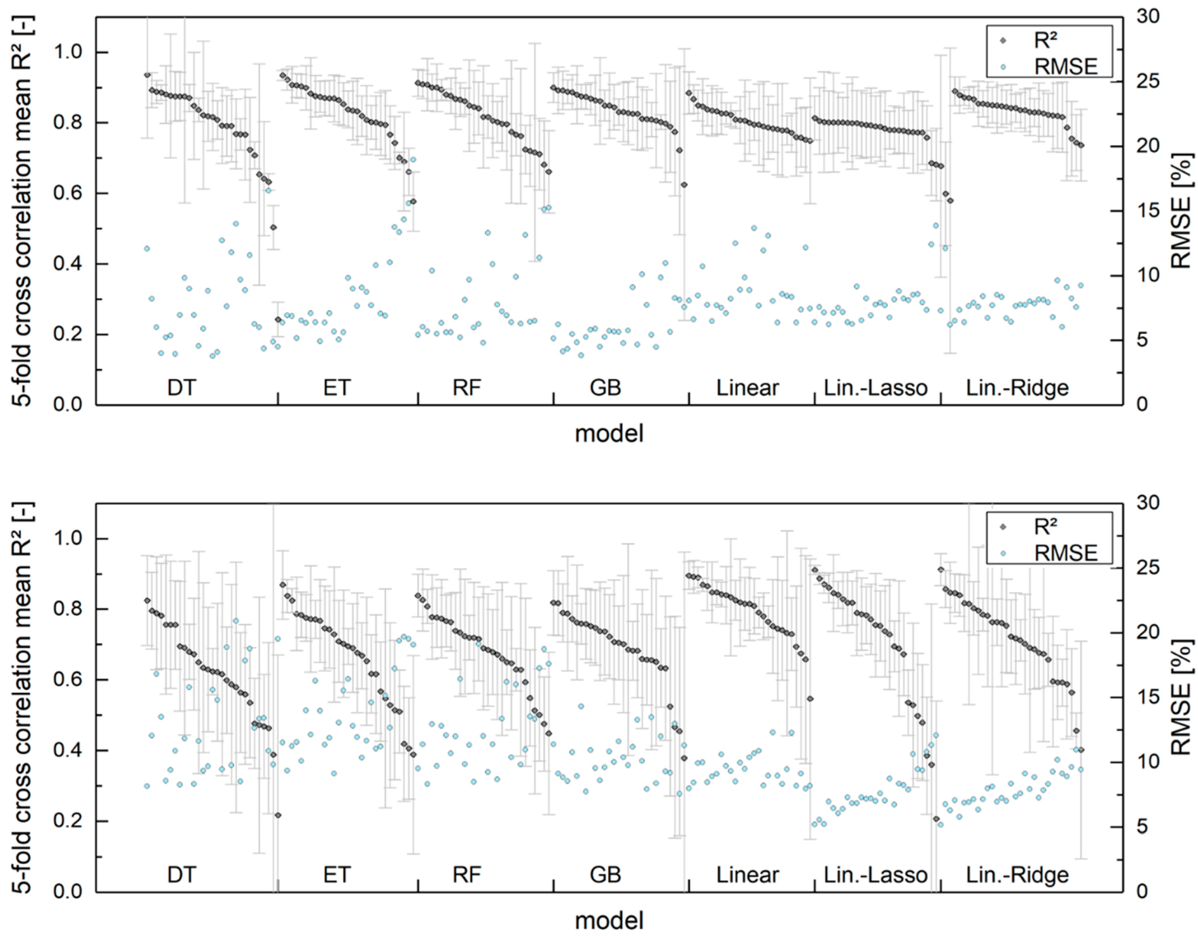
Figure 6 displays the result of the training process for both feature vectors (histogram- and texture-based) using different regression models and model parameters for models based on all 9 fuel mixture classes. The average 5-fold cross validation
R2 and the RMSE serve as evaluation criteria. The plot is divided into model-specific subsections, which are internally sorted by the
R2 value based on the validation data set. In general, both feature vectors are, in combination with a properly trained model, capable of reaching high predictive accuracy with
R2 > 0.8. The corresponding RMSE values lie below 10% (in units of mixture fraction or fuel quality). The best histogram-based model leads to a RMSE of 3.8% (DT model) for unknown validation data and the best texture-based one reaches 5.1% (Linear Lasso). Overall, the histogram-based approach exhibits higher accuracies and lower errors. It furthermore shows a lower discrepancy between the best and worst models of similar kind. This will be discussed in the following sections with respect to the model parametrization, input data selection and the training strategy.
3.1. Influence of Regression Model and Parametrization
Although most of the examined models display potentially high predictive accuracy, there are substantial differences. These, and their origin, will be discussed in this section, based on the training process with all nine fuel-mixture classes.
For all of the regression algorithms, there are both accurate and flawed models, as displayed in
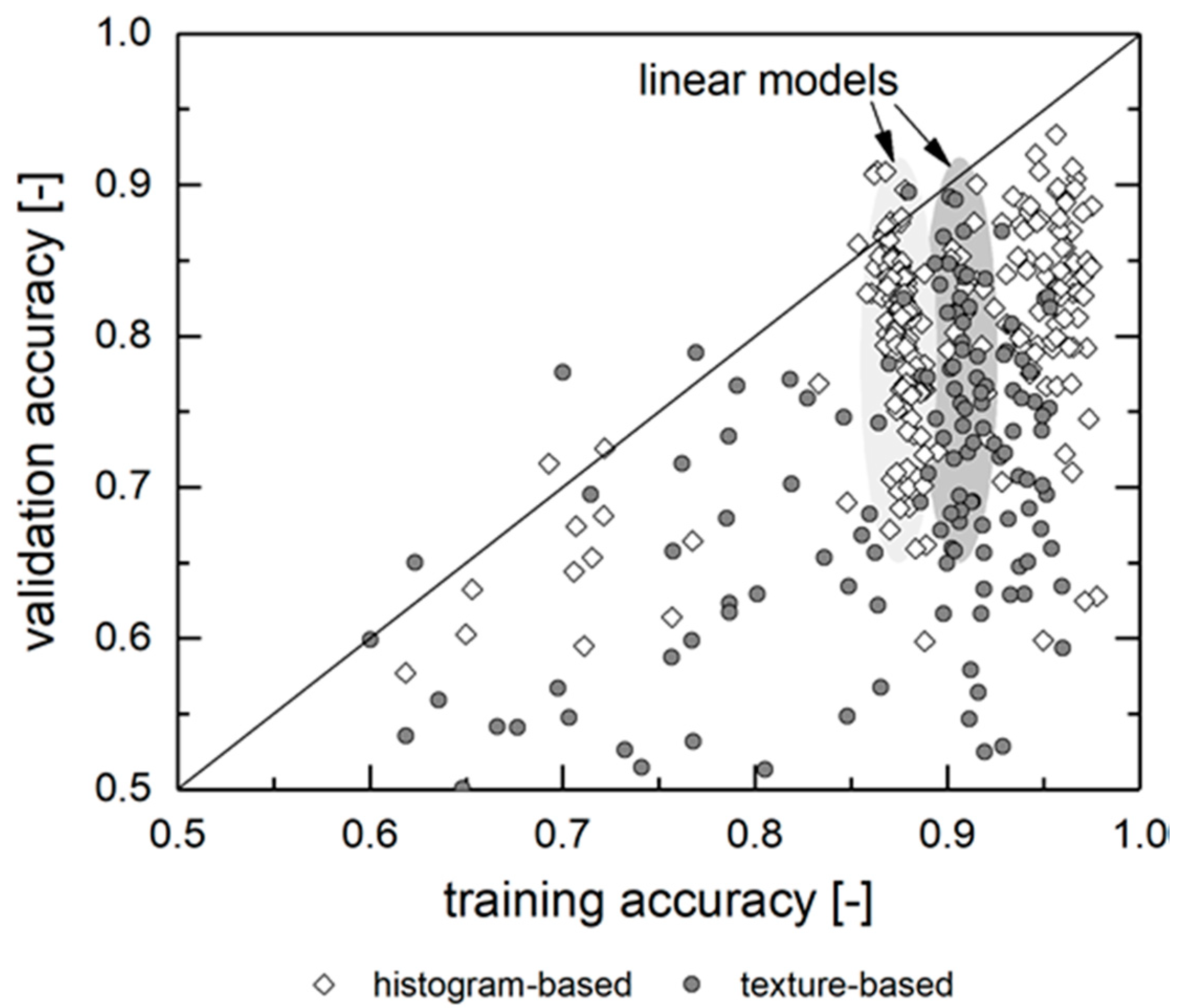
Figure 6. At first glance, this could be due to the model parametrization (e.g., boundary conditions, such as the adaboost algorithm, the deepness of the tree models or the regularization factor α). However, the evaluation shows that the parametrization does not explain most of the deviances (albeit it plays an important role for some models, which will be discussed later). Most of the models are robust to parametrization. Instead, these models’ performances heavily rely on the training process itself. This can be assessed by comparing a model’s training and validation accuracy.
Figure 7 displays this relation. Unsurprisingly, models with low predictive quality after the model training fail during the validation process as well. However, there are dysfunctional models with high training accuracy as well, especially for the histogram-based models with tree-type regression.
The training accuracies of the linear models are generally lower than one of the best performing tree-type models, yet they are more stable, with the R2 lying in the range of 0.87 ± 0.006 for the histogram-based approach and 0.90 ± 0.007 for the texture-based approach. However, regarding the validation accuracy, many of these models are outranked by the best performing nonlinear models. When well-trained linear models exhibit low validation accuracy, this is due to a non-representative (or insufficient) provision of training data or due to an underfitted model. Indeed, the bias–variance decomposition shows a trend towards lower variances and higher bias for the underperforming linear models during validation. Consequently, the model either encounters unknown (as in “never seen before”) features during validation or features that did not find representation in the model parameters βi. The first factor can be addressed by increasing the amount or quality of training data (or at least the share used for training); the latter by using more complex regression models, such as the tree-type models.
For these, including their boosted and bagged derivates,
Figure 6 also depicts a big discrepancy regarding the prediction accuracy. There are both high and low quality predictions for each individual model, depending on the training process. The histogram-based approach leads to higher accuracies on average, as well as for the individual best model in comparison to the texture-based approach. The difference in the
R2 value amounts for 0.06–0.1. The adaboost algorithm improves the median accuracy by 0.03–0.10 for histogram-based regression. For texture-based regression, the median improvement is higher up to Δ
R2 = 0.20 for the DT model. This is due to the DT model being the only non-ensemble model, thus gaining the largest benefit from the boosting algorithm. In all cases, there is also no correlation of
R2 and the number of estimators. Increasing the trees deepness affects the prediction accuracy only for values up to 4. Higher values increase the computational needs without improving the accuracy. We consequently suggest choosing parameters leading to shorter calculation times (e.g., a limited number of tree layers (up to 4) and adaboost estimators (up to 200)).
Consequently, most of the examined regression models could theoretically be used for the real-world application of fuel recognition. Parametrization and, in particular, training, require an individual adaption and testing of the underlying model.
Table 2 and
Table 3 give an overview of the results obtained by the different regression algorithms.
3.2. Influence of the Training Data
As displayed, the high discrepancy between the best and the worst models—for both linear and tree-type models—is not the result of improved hyperparameter tuning, but the result of the images/input data used for training. The most influential factor for an individual model is the (random) selection of training and validation data. This becomes apparent when taking the standard deviation of the k-fold cross-validation
R2 into account (cf. the error bars in
Figure 6). Depending on the (random) choice of the training folds, the regression leads to models of different predictive capabilities. While some trained subsets reach standard deviations of as low as 0.02 regarding
R2, certain models feature values of 0.2 or more; in these cases, the training results in flawed and insufficient models.
There are two major issues regarding the input data, leading to underperforming models:
First of all, the amount of training and validation data may be insufficient for this kind of problem. Depending on the random samples used for training and testing, the model then encounters either simple/known or unknown data/outliers. This could be addressed by drastically increasing the amount of input images and utilization of more complex models. However, this also risks overfitting and highly biased models.
On the other hand, the input images—more precisely, the applied image labels—might be misleading, and the source of errors as well. The manual fuel preparation, mixing and, most importantly, the image capturing process definitely affect the training process. The camera’s limited point-of-view probably results in images (and, subsequently, histograms and Haralick features) that are not perfect representatives of a certain class, albeit they are labelled as such. Besides the inhomogeneity, the fuel’s lumpiness also plays a role. For instance, large chunks of bright wood chips—that appear in the low-quality FR as well—will affect the predictions, shifting the results towards higher predicted quality, while patches with typically darker fine particles shift the prediction towards lower qualities. In addition to that, certain training classes lie close together (e.g., 25/75, 33/66 and 40/60 with only 7–8% deviation in fuel quality) so that the statistic error of sampling and image capturing lies in the same order of magnitude as the applied labels.
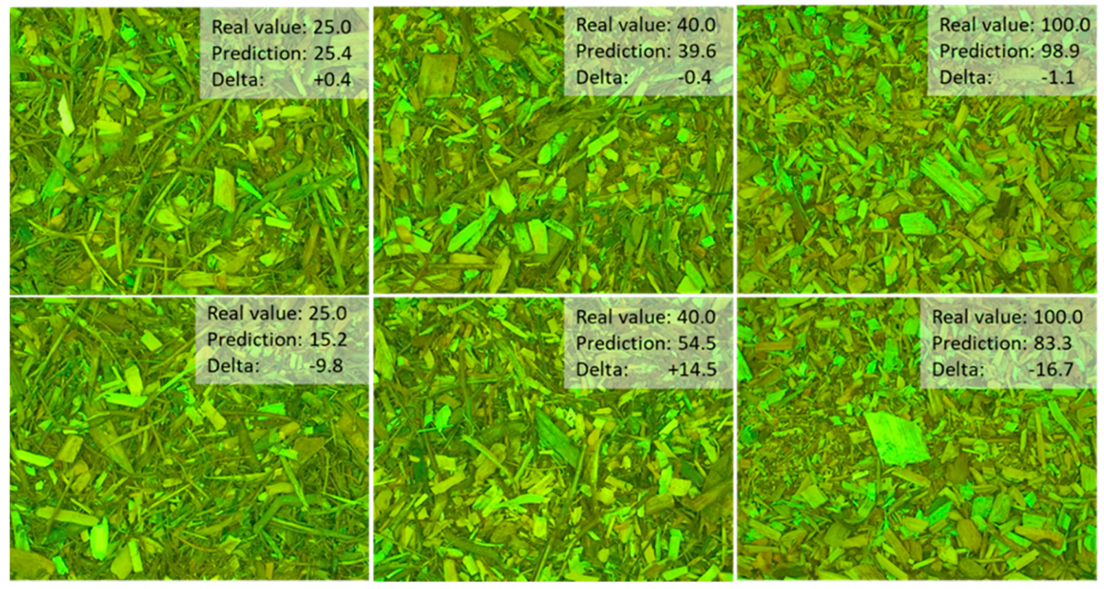
Figure 8 shows some examples of prominent model failures for irregular images and respective photos with high accuracies. The flawed prediction of the 25/75 photograph in
Figure 8 (left) visually appears to be darker than the correctly assigned prediction. The source of the error thus lies in the sampling process, not in the modelling itself.
Yet, with regard to the intended use, these kinds of errors must be accepted. Due to their size and a flawed mixing process, the targeted application thus faces similar challenges (i.e., fluctuating qualities, difficult validation and a limited field-view and point-of-view onto the surface of the feedstock material). Training with images taken from megawatt-scale industrial furnaces will consequently always suffer from similar drawbacks.
3.3. Influence of the Training Strategy
As mentioned, the training process in full-scale environments is challenging. Due to the yard-“mixing” of several cubic meters of feedstock with bulldozers in biomass power plants, training a model with exactly determined pairs of images and data labels (i.e., quantified defined mixture classes) is an impossible task. As described above, for this reason, we performed model training with a reduced amount of data and labels. The most elementary model relies on a two-point training process with pure WC and FR, respectively. This means that the whole range of possible mixtures relies on the interpolation capabilities of the underlying regressor.
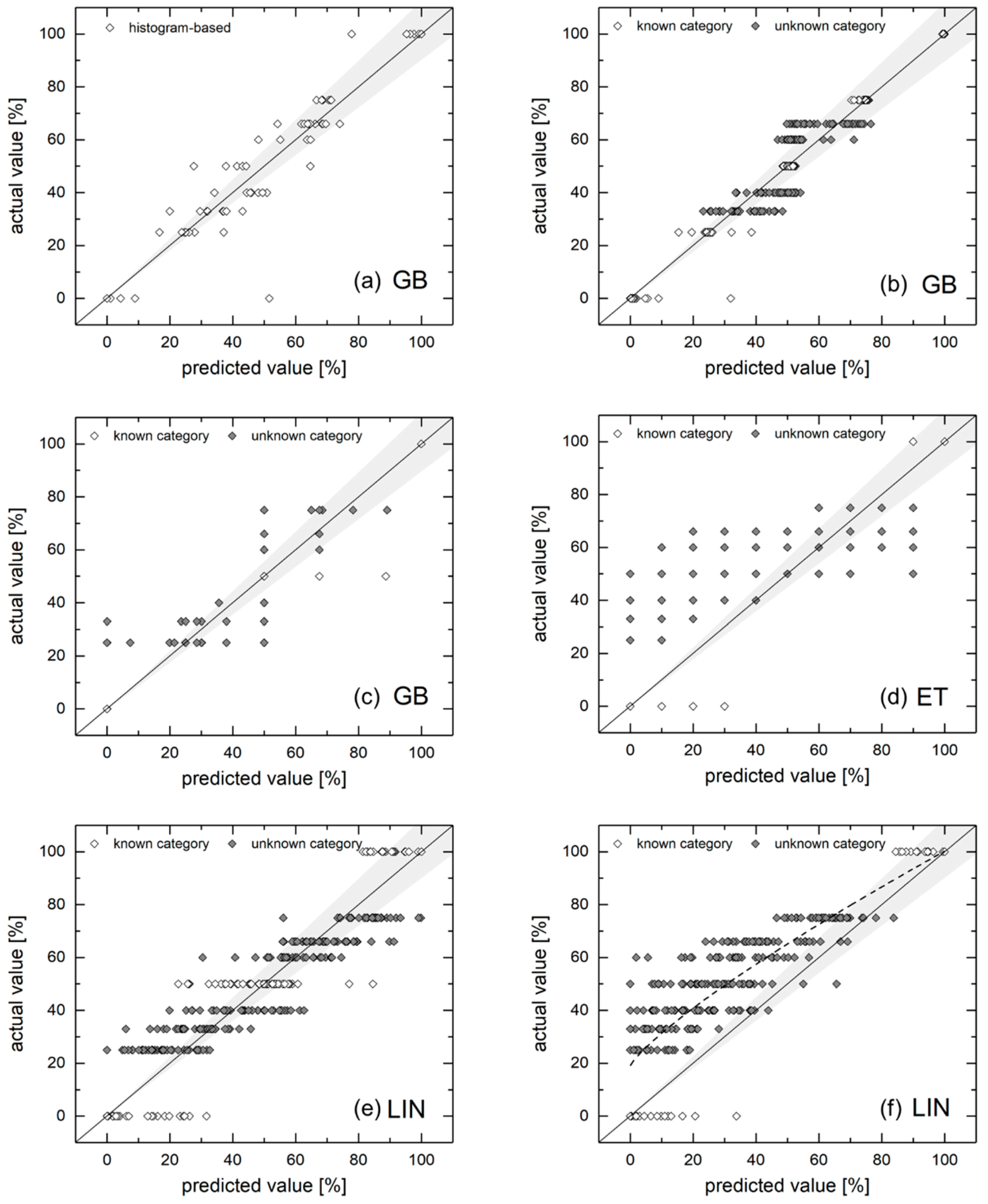
This section’s analysis relies on the histogram-based feature vector. As models, we used a reduced selection of algorithms: GB due to its robustness, ET due to its enhanced interpolation capabilities (because of the random splits) and the adaboosted linear model for simplicity.
Figure 9 displays the corresponding results by comparing predicted and actual mixture fractions. Graph (a) shows a GB reference case, in which all 9 classes were used for training. In contrast, graph (b) relies on five distinct classes (shown in white), while the other categories (dark dots) are subject to interpolation. It becomes apparent that this model performs better for known classes. The standard deviation for the predictions lies in the range of σ = 0.22–5.60% (for fuel quality) around their average value for these classes. Unknown ones lie in the range of σ = 4.68–8.32%. However, the confidence of predictions can be enhanced by providing a sampling size n > 1. The sample size n could be increased—even in the envisaged application in industrial furnaces—by capturing and evaluating several different photos of an unknown fuel mixture. This mitigates the risk of capturing a non-representative sample and, furthermore, reduces the model’s prediction uncertainty.
The necessary minimum sample size of images n can be approximately estimated from the standard deviation σ according to Equation (8) under the assumption of normally distributed values [
33]:
z depends on the desired level of confidence. For 90% confident predictions,
z equals
z = 1.645 and it rises for higher levels, (e.g.,
z (95%) = 1.96).
e represents the acceptable (margin of) error. This means that n different photos of a distinct fuel are necessary in order to estimate its fuel quality with a confidence of 90% (
z = 1.645), while allowing an estimation error of up to
e = 10 [%].
If all 9 classes are used for training, only a few samples are required: In order to reach a 90% confident prediction, this corresponds to sample sizes of up to 5 (for the worst case σ = 8.32 and an acceptable error of 6 [%]). However, for σ = 5 and an acceptable error in fuel quality deciles (e = 10 [%]), one sample is still sufficient for 95% confident predictions.
For a reduced number of classes, as shown in graphs (c) and (d), as models trained with three and two classes, respectively, the error significantly increased. Although these algorithms (GB and ET) tend to deliver predictions scattering around the suggested real values, standard deviations of σ > 15 hinder accurate predictions, even for higher samples sizes n > 10. Since one has to keep the other sources of errors and uncertainties mentioned above in mind, only trends can be assessed by these approaches.
However, graphs (e) and (f) show the results obtained from a similar training strategy, but this time using the linear regression. In these cases, predicted values scatter more densely around the real mixture values, the maximum standard deviation of graph (e) (three-class training) equals σ = 11.99 around their mean value for the 50% fuel quality class. This corresponds to a sample size of n ≥ 3.47 in order to obtain a 90% confidence for a certain fuel quality decile (e = 10 [%]). The two-class training approach requires only slightly higher sample sizes. However, in this case, the interpolation does not follow the desired linear relation between 0 and 100% fuel quality. Consequently, fitting the underlying trend (cf. the dotted line in graph (f), a fitting curve according to the Equation y = a + bxc) ought to be applied in order to obtain real mixture values.
3.4. Repercussions for the Industrial Application
Although not perfectly accurate, the two- and three-class training, based on the linear regression algorithm sound promising in order to continuously assess the fuel (mixture) quality, even in full-scale environments. Consequently, the training process of such a system could even be performed in the ongoing operations of a biomass furnace. The system’s calibration may happen during two short-term runs with unmixed, pure fuels of both kinds, potentially complemented by training data from a typical 1:1 mixture. Subsequently, the required sample sizes for approximate predictions lie in a range of n < 5, which can be easily obtained by continuously monitoring sliding floors, conveyor belts or chain conveyors in biomass plants with camera systems and appropriate lighting. Since capturing and evaluating an individual photograph of feedstock on current standard office hardware requires significantly less than 1 s, the system can be used in order to capture live data. When special attention is paid to the hardware and optical systems, higher sampling rates are certainly possible as well.
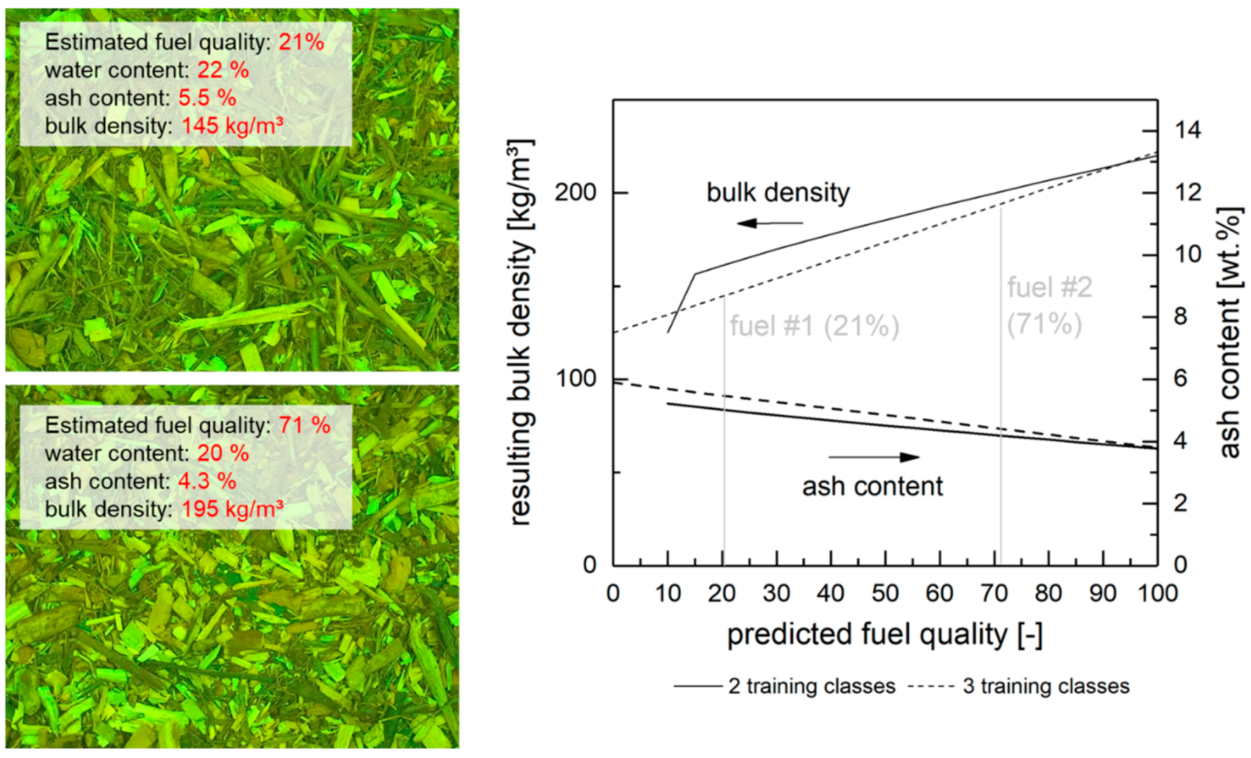
Finally,
Figure 10 displays the potential application of the methodology in order to calculate fuel properties from predicted mixture ratios by either applying linear interpolation (which, as discussed, is appropriate when using more than two fuel classes of training images) or a modified relation between the predicted and actual fuel quality. The latter has been demonstrated in
Figure 9, graph (vi) for the two-point calibration. The underlying assumption of a linear behavior of fuel properties (e.g., bulk density), seems valid. As shown in
Section 2.1, a mixture (1:1) of WC and FR exhibits approximately the mean value of both fuels.
4. Summary and Conclusions
This article examines and demonstrates a method for the assessment of fuel properties to identify the volumetric mixture fractions of two types of wood biomass. The approach is designed with respect to an envisaged application in industrial biomass furnaces and power plants. We assess the influence of different sources of errors and uncertainties during our lab-scale examinations in order to gain knowledge about the system’s properties and repercussions for operation in full-scale environments. We apply two different kinds of image processing techniques to generate feature vectors (a spatial/texture-based and an integral/histogram-based one) for regression modelling. Wood chips and forest residues in nine distinct mixture fractions serve as feedstock. Subsequently, we examined seven regression algorithms with different parametrization, including ensemble models, such as boosting and bagging.
This approach leads to a series of conclusions:
Both histogram- and texture-based modelling approaches are capable of identifying fuel mixture qualities with an acceptable error. Especially for the first, the obtainable accuracy (as R2) values are larger than 0.90. Furthermore, models based on histogram features are more robust to subpar training compared to texture information. The generally most reliable results were obtained by the gradient boosting (GB) models and the linear model for both feature vectors, as mirrored in the low RMSE values of their predictions.
The application of the adaboosting algorithm enhances the median model accuracies by values of ΔR2 = 0.02–0.04 for the histogram-based and up to ΔR2 = 0.15–0.20 for the texture-based feature vector. L1/2 regularization improves the linear models’ accuracies, especially for the texture-based regression (for 10−5 < α < 10−4) and has close to no effect on the histogram-based models.
The data preparation and training process are the principal reasons for underperforming models and require the most attention during model preparation. Especially the image labelling (i.e., assigning a class to images and/or providing training images with exactly determined properties) is challenging for lab-scale considerations and even more so for the target purpose in industrial furnaces.
It is possible to train models relying on a reduced amount of distinct classes, interpolating in between. Although the predictive accuracy significantly shrinks when using three instead of nine mixture classes during the training process, we find that it is still possible to obtain reliable predictions, even for sample sizes n < 5. This enables us to reliably distinguish fluctuations of 10% in the fuel mixture quality. If not otherwise possible, even a two-point calibration is applicable to continuously monitor feedstock quality, consequently, still revealing otherwise unobtainable information. In this case, a linear model should be used due to its better interpolation capabilities.
All in all, this work describes and examines a series of steps, considerations and prerequisites in order to develop and train an optical regression-based system for the online detection of fuel quality prior to the actual combustion process. This method is thus potentially capable of improving the furnace’s process control with respect to fluctuations in feedstock quality by behaving proactively, rather than reactively. More precisely, the gathered information (here as “fuel quality” correlating with the feedstock’s volumetric density) can be used to optimize a grate furnace’s fuel stoker. The developed methodology will be subsequently implemented into a biomass heat and power plant in the megawatt range in order to gain further operational knowledge, identifying and quantifying its potential during long-term operation.
Future work should address other relevant fuel properties, potentially derivable from images, such as particle size (distributions), fine particle content or the content of mineral soil and further contaminations.


