Abstract
This paper presents a multi-scale-homogenization based on a two-step methodology (micro-meso and meso-macro homogenization) to predict the elastic constants of 3D fiber-reinforced composites (FRC). At each level, the elastic constants were predicted through both analytical and numerical methods to ascertain the accuracy of predicted elastic constants. The predicted elastic constants were compared with experimental data. Both methods predicted the in-plane elastic constants “” and “” with good accuracy; however, the analytical method under predicts the shear modulus “”. The elastic constants predicted through a multiscale homogenization approach can be used to predict the behavior of 3D-FRC under different loading conditions at the macro-level.
1. Introduction
The use of 3D fiber-reinforced composites (3D-FRC) has been increasing in recent years, thanks to their superior delamination resistance, multi-directional load-bearing capacity and transverse properties [1]. The physical testing of these composites is not only expansive but also time-consuming. However, with developments in computer processing capacity, virtual testing of FRC is one of the main interests among academics and industry in this field. Due to the complex fabric architecture of 3D-FRC, the accurate prediction of their elastic constants is a challenging task. Several models have been proposed to predict the elastic constants of these novel 3D fabric architectures. These models are broadly divided into analytical [2,3,4,5] and numerical [4,6] models.
The analytical models are used to predict the homogenized properties of 3D-FRC, which are based on classical laminate theory (CLT) coupled with iso-stress/iso-strain assumption. These models give a reasonable estimation of in-plane properties; however, they over-predict the out-of-plane and shear constants. The finite element (FE) method based numerical models have been widely used to predict the elastic constants of 2D and 3D-FRC [7]. In comparison with analytical models, numerical models give a better prediction of elastic constants and stress/strain field distribution. However, the FE analysis of 3D-FRC requires computational cost and time to model complex fabric architectures. The elastic constants of 3D-FRC depend on many parameters such as the fiber volume fraction and volume proportion of each yarn and the arrangement of yarns in the weave architecture. The accuracy of the predicted effective properties depends on the accuracy of the geometric parameters and the definition of representative volume element (RVE) as close as possible to real weave architecture. The numerical models can efficiently accommodate more complexities than analytical methods; however, they are computationally very expansive. Nevertheless, the analytical models are quick, especially in the case of the parametric study, and they are reasonably accurate in predicting the elastic constants.
The FE analysis of 3D-FRC can be performed at a micro level, meso level [7], macro-level [8,9], and a combination of different levels called multiscale analysis [10]. The FE analysis at each level requires a complete set of engineering elastic constants of all constituents, i.e., at a micro level, the properties of fiber and matrix are needed; at the meso level, the properties of impregnated tows and matrix are required, and at macro level homogenized properties in term of nine engineering constants are required. Due to the complex weave architecture of 3D-FRC, their FE analysis at the micro and meso level is not feasible for large composite structures, i.e., yachts, wind turbine blades, airplane fuselage etc. Therefore; for such cases, macro-level FE analysis is preferred. The accuracy of the FE analysis depends on the engineering elastic constants of 3D-FRC. To experimentally determine all the engineering constants is a challenging task. Therefore, researchers take advantage of analytical and numerical methods to predict effective properties and compare them with benchmark values.
In this paper, both numerical and analytical approaches have been used to predict the properties of 3D-FRC. The predicted values are then compared with the experimentally determined warp modulus “”, weft modulus “” and shear modulus “” values. The predicted elastic constants can be used to predict the behavior of 3D-FRC under different loading conditions. The prediction of elastic constants using numerical or analytical methods, requires accurate definition of internal geometry and fiber volume fractions of each tow are very critical, which will be discussed in the following section.
Multiscale Homogenization of 3D-FRC
The 3D-FRC possesses a higher degree of heterogeneity as compared to the 2D FRC (unidirectional and bidirectional), due to be their complex weave architecture. The intricate architecture makes 3D-FRC difficult to characterize, and their behavior under different loading conditions is equally challenging to predict. The effective properties of 3D-FRC depend on the volume proportion of each constituent (fiber and matrix) and fabric architecture. In multiscale modeling, 3D-FRCs are divided into three structural levels, i.e., micro-level (individual fiber and matrix within each yarn), meso level (individual yarn and matrix in RVE) and macro-level (orthotropic material having different elastic constants in all three directions), as shown in Figure 1.
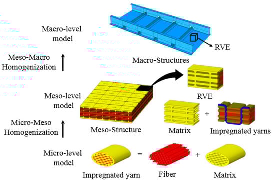
Figure 1.
Multiscale modeling and homogenization in 3D fiber-reinforced composites (3D-FRC).
Multiscale modeling shows how these three levels interact with each other, i.e., mechanical properties at the macro level depends on the properties of the meso level element (impregnated yarns and matrix), and the properties of impregnated yarns depend on the properties of the micro-level element (individual fiber and matrix).
In most of the cases, the micro-level and meso level approaches mentioned above are computationally very expansive and possess limitations in analyzing full-scale problems. Therefore, it is recommended to use homogenized macro-level models while analyzing 3D-FRC to solve real problems through numerical simulation. The process of predicting the equivalent material properties of 3D-FRC is called homogenization. The equivalent material properties can be determined through analytical and numerical methods based on a multiscale approach, i.e., using the constituent’s properties at the micro/meso level to determine macro-level effective properties. In this work, a two-step multiscale based homogenization approach is presented to predict the effective properties of 3D-FRC. In the first step (micro-macro homogenization), the effective properties of impregnated yarns were calculated through constituent properties (fiber and matrix). Whereas, in the second step, the engineering elastic constants of 3D-FRC were determined using effective properties of impregnated yarns, determined in the first stage of homogenization.
Using the multiscale homogenization approach mentioned above, the 3D-FRC is converted into equivalent 3D orthotropic ply, as shown in the schematic diagram shown in Figure 2. The figure shows the normal and shear stress components acting at each integration point in an orthotropic ply. It is important to note that stresses and strain distribution in the actual meso level models or in simplified RVE are not homogenous due to the difference in the stiffness of fiber and matrix. The stiffness of the matrix is 20–50 times smaller than fiber; as a result, the matrix undergoes large deformation as compared to fibers, especially in the case of matrix dominant loading. The FRC is heterogeneous in nature, and it is recommended to consider average stress and strains acting on a volume element (RVE). The average stresses “” and resulting average strains “” at each integration point of volume element are given by Equations (1) and (2) respectively. Hence, all the mechanical properties of 3D-FRC are calculated based on average stresses and strains acting on the volume element.
where “V”, “” and “” represents the volume of element, stress tensor, and strain tensor, respectively.
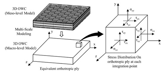
Figure 2.
The equivalent orthotropic ply of 3D-FRC.
2. Materials and Methods
2.1. Materials and Fabrication Process
The 3D fabric used in this study is 3D orthogonal E-glass woven fabric (3D-9871), supplied by TexTech industries, USA. The density of the 3D fabric used is 5200 g/cm2. It consists of three layers of warp yarn and four layers of fill yarns, as shown in Figure 3. The cross-section area of middle warp yarn is twice the size to maintain the same in-plane properties along both directions (warp and fill). The fabric contains 49% of yarns along the warp and fill direction, whereas only 2% yarns were present along the z-direction to bind the in-plane yarns together. The linear density of warp and fill yarn is 2.8 and 1.9 end/cm, respectively. The epoxy resin Epolam® 5015/5015 from Axson, USA, was used to fabricate 3D-FRC. The epoxy to hardener ratio used to fabricate the 3D-FRC panel was 100:30 by weight. The 3D-FRC was fabricated using a vacuum-assisted resin infusion process. After resin infusion, the composite panels were post-cured in an oven for 8 h at 80 °C, to achieve maximum mechanical properties. The overall thickness of a cured panel is 3.96 mm.
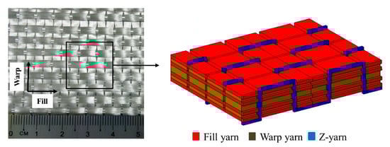
Figure 3.
3D orthogonal fiber-reinforced composites.
2.2. Mechanical Testing of 3D-FRC
The elastic constants predicted through analytical and numerical methods were validated through experimentally determined benchmark values. The mechanical tests have been conducted to determine tensile modulus along the warp and fill direction, and in-plane shear modulus. The tensile and V-notch shear test was performed according to ASTM D3039 and ASTM D7078 standard, respectively. For the tensile test, rectangular samples of 250 mm × 25 mm in dimension were cut along the warp and fill direction from the post-cured 3D-FRC panel. Whereas 56 × 76 mm rectangular samples were prepared for the V-notch shear test. The tests were conducted at a load rate of 1 mm/min on Zwick Roell 50 kN load frame. Five samples were tested for each test, and average values were calculated.
2.3. Geometric Parameters of 3D-FRC
The geometric parameters of an individual yarn (height and width of yarn) and RVE (length, width, and height of RVE) were determined from the fabricated pane. Figure 4a shows the optical images of a cross-section along the warp and fill direction. The geometric parameters obtained from optical images using an optical microscope are given in Table 1. This step is essential because the non-representative geometric parameters lead to a significant error in the prediction. The idealized geometric model of RVE has been developed through measured weave parameters, as shown in Figure 4b.
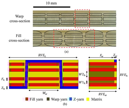
Figure 4.
The geometry of 3D-FRC along with parameters: (a) optical images of the fabricated panel; (b) schematic diagram showing weave parameters of 3D-FRC.

Table 1.
Geometric parameters of 3D-FRC.
2.4. The Fiber Volume Fraction of Impregnated Yarns
The elastic constants of impregnated yarns depend on the fiber volume fraction and cross-sectional area. In this work, the fiber volume fraction was calculated using the linear density of yarns, also called Tex-count (g/km), given by Equation (3). The linear density was determined for each yarn, which is given in Table 2. The fiber volume fraction of each yarn was calculated through the linear density and cross-sectional area of each yarn. It was then used to determine engineering elastic constants of individual impregnated yarns. The fiber volume fraction of each yarn is given in Table 2.
Table 2.
Fiber volume fraction of yarns.
2.5. Micro-Meso Homogenization
At micro-level, each impregnated yarn (warp, fill, and z-yarn) was considered as unidirectional ply. The stiffness constants and engineering elastic constants of yarns (impregnated yarns) were calculated from constituent properties, i.e., elastic constants of fiber/matrix and the fiber volume fraction. The elastic constants of E-glass fiber and epoxy matrix are given in Table 3. The matrix was considered as isotropic; whereas, impregnated yarns were considered as transversely isotropic material arranged in three perpendicular directions. The fiber volume fraction of yarn was about 70%, calculated using a linear density of fibers and cross-sectional area of yarns, as explained in the earlier section. The homogenized elastic constants of yarns were predicted using both analytical and numerical methods, which are explained in the following section.
Table 3.
Elastic constants of fiber and matrix.
2.5.1. Analytical Method
The Chamis [7] model was adopted to calculate the homogenized effective properties of transversely isotropic material, i.e., impregnated yarns. The authors proposed micro-mechanical relationships to calculate the elastic constants of yarns, given by Equations (4)–(8).
where, “” “” “” and “” represent the fiber volume fraction, Poisson’s ratio, modulus of elasticity, and modulus of rigidity of the fibers. The constants “” “” and “” represent the Poisson’s ratio, modulus of elasticity and modulus of rigidity of the matrix and the constants “”, “”, “”, “”, “”, “”, “”, “” represents the effective modulus of elasticity, modulus of rigidity, and Poisson’s ratio of the impregnated yarn in local coordinate systems (1,2,3).
2.5.2. Numerical Method
The unit cell approach is a proven method to predict the elastic constants of FRC through the numerical method. In actual FRC, the fibers are randomly distributed inside the impregnated yarns (unidirectional FRC), in the form of locally aggregated fibers and resin pockets [11]. Several authors used idealized fiber packing (triangular, square, diamond or hexagonal) to predict the elastic constants of unidirectional FRC. In this study, it is assumed that the impregnated yarns contain idealized hexagonal fiber packing or fiber arrangement. This repetitive hexagonal unit-cell is uniformly distributed inside yarn [8]. The homogenized elastic constants of impregnated yarns were determined using 3D hexagonal unicell, as shown in Figure 5a. In addition to the random distribution of fiber, the fiber diameter also varies. Typically, E-glass fiber diameter varies between 10–20 μm. In this study, a constant diameter of E-Glass fiber is assumed for micro unit-cell, i.e., 15 μm. The dimensions of a unit cell can be calculated through fiber volume fraction “” and radius of a fiber “”, using Equation (9), where constants “”, “” and “” represent the dimensions of the unit cell, as shown in Figure 5a. Based on fiber radius (7.5 µm) and fiber volume fraction (70%), the dimensions of the unit cell are , and . The unit cell was meshed with eight-node solid elements (C3D8R), as shown in Figure 5b.
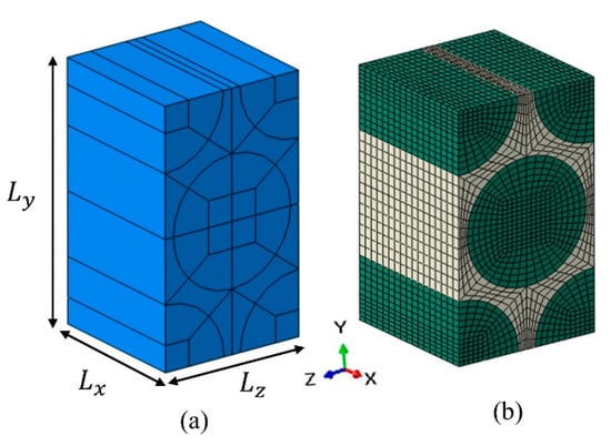
Figure 5.
Hexagonal unit cell: (a) parameters of a unit cell, (b) meshed unit cell.
The main objective of a unit cell is to determine the compliance coefficients of a material. For this purpose, periodic boundary conditions are required, so that a single repetitive unit-cell can mimic the behavior of entire unidirectional composites. To evaluate the elastic constants of unidirectional composite, a set of six different load cases were considered to ensure periodicity in all directions. The periodic boundary conditions consist of three normal strains and three shear strains of load vectors, which are given in Table 4. The elastic of fiber and matrix used is given in Table 3. Based on the boundary conditions, the FE analysis was run for each load case (six FE analysis) to evaluate the homogenized stiffness matrix of a unit cell. The compliance matrix was then calculated by taking the inverse of the stiffness matrix given by Equation (10). Finally, the homogenized properties of a 3D hexagonal unit cells in local coordinates were evaluated from a compliance matrix using Equation (11).
Table 4.
Periodic boundary conditions for different load cases.
2.6. Meso-Macro Homogenization
In the meso-macro homogenization, the geometry of 3D-FRC as close as possible to actual architecture is required. The fabricated 3D-FRC shows rectangular cross-sections; the geometric parameters are given in Table 1. The idealized geometry of 3D-FRC was generated to predict the homogenized elastic constants. To ascertain the accuracy of elastic constants, both analytical and numerical methods were used, which are explained in the following section.
2.6.1. Analytical Method
The analytical method used in this work is based on the volume averaging method [2,12,13], which uses realistic internal geometry. In this method, the engineering elastic constants of 3D-FRC were calculated using elastic constants and the volume proportion of each constituent in the RVE. The RVE represents the repeated element at the macro level, representing the entire 3D-FRC. The overview of the volume averaging method is given in Figure 6. The homogenized elastic constants of impregnated yarns in the local coordinate system (1,2,3) predicted using micro-meso homogenization, were used to predict the engineering elastic constants of 3D-FRC. These local stiffness matrices of each yarn were then transformed with respect to the global coordinate system (x, y, z) to get transformed stiffness matrix of each yarn in RVE. The volume proportion of each constituent in the RVE was determined from the geometric model of 3D-FRC, which are given in Table 5.
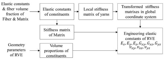
Figure 6.
Flow chart showing steps of volume averaging method.
Table 5.
Volume proportion of impregnated yarns.
After evaluating the volume proportion of each constituent “” and transformed stiffness matrixes in the local coordinate system “”, the volume averaging method was then applied to calculate the stiffness matrix of RVE, according to Equation (12). The engineering elastic constants of RVE were calculated by taking the inverse of the global stiffness matrix of RVE, given by Equation (13). Finally, the elastic constants of 3D-FRC were calculated using Equation (14). For the detailed procedure, on how to apply the volume averaging method, the readers are requested to follow the references [1,2,3].
2.6.2. Numerical Method
In the finite element modeling approach, the engineering elastic constants of 3D-FRC were predicted using the meso-macro homogenization approach, i.e., the RVE of 3D-FRC was assumed to have homogenized properties at a macro level. The meso level geometry of RVE of 3D-FRC is shown in Figure 7. All the yarns were modeled with a rectangular cross-section area. Python code was used to generate the FE model along with boundary and load conditions in Abaqus. The finite element model consists of tetrahedral solid elements (C3D8R). The elastic constants of 3D-FRC were predicted through periodic boundary conditions, which are given in Table 4. The FE analysis was run for each periodic boundary condition to evaluate the homogenized stiffness matrix of RVE, . The compliance matrix was then calculated by taking the inverse of the stiffness matrix given by Equation (13). Finally, the engineering elastic constants of 3D-FRC were evaluated from a compliance matrix using Equation (14).
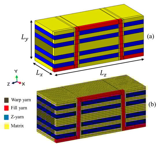
Figure 7.
Representative volume element (RVE) of 3D-FRC, (a) geometry of 3D-FRC along with parameters, (b) meshed geometry of 3D RVE.
3. Results and Discussion
In the case of micro-meso homogenization, the summary of homogenized elastic constants of impregnated yarns predicted through the analytical and numerical method is given in Table 6. The longitudinal moduli (, ,) and Poisson’s ratio ( and ) predicted by both methods were close to each other. However, transverse Poisson’s ratio () and shear moduli (, and ) show up to 8.5% and 6.5% difference in the prediction. The predicted elastic constants of yarns (unidirectional composites) through micro-homogenization is based on idealized hexagonal unit-cell model. The effect of local fiber aggregation, random distribution of fibers, resin-rich pockets, voids, variation in fiber diameter and fiber misalignment due to the undulation of z-binder were ignored [11,14]. All these factors may affect the predicted elastic constants of 3D-FRC at macro-level.
Table 6.
Summary of elastic constants (impregnated yarns).
In the case of meso-macro homogenization, the homogenized elastic constants of 3D-FRC predicted through analytical and numerical methods are given in Table 7. It also shows the comparison of numerical/analytical results with the experimentally determined elastic constants through in-house testing, i.e., elastic modulus along warp direction (), elastic constant along fill direction () and in-plane shear modulus (). The results highlight that the in-plane elastic constants predicted through the analytical and numerical models are in close agreement with the experimental values. In the case of analytical prediction, the longitudinal ( and ) and shear modulus () shows 4.1% and 9.5% error, respectively. Whereas, in the case of numerical prediction the percentage error in the longitudinal ( and ) and transverse shear modulus (Gyz) is ~1.5%, and ~6.2%, respectively, between experimental and numerical results. The numerical prediction is closer to the actual elastic constants because it can accommodate more geometric variabilities and actual boundary conditions. The predicted elastic constants can be used in the finite element analysis of 3D-FRC structures at a macro level, under different loading conditions.
Table 7.
Summary of elastic constants (3D-FRC).
4. Conclusions
A multiscale homogenization method has been implemented to predict the engineering elastic constants of 3D-FRC. The method consists of two-steps, i.e., micro-meso homogenizations and meso-macro homogenization. The elastic constants predicted through analytical and numerical methods were compared with the benchmark experimental values. In the case of micro-meso homogenization, both analytical and numerical models show a low variation in the predicted elastic constants. The maximum difference between the analytical and numerical models is in the Poisson’s ratio “” and shear modulus “” up to 8.5% and 6.5%, respectively. In the case of meso-macro homogenization, the percentage error between analytical prediction and experimentally determined values were up to 4%, for longitudinal “” and transverse “” modulus and 9.5% for shear modulus “”. In comparison, the numerical model shows up to 1.5% difference for longitudinal “” and transverse “” modulus, and 6.2% difference in shear modulus “”, with experimental data. Both analytical and numerical model prediction shows good agreement with experimental data. However, the numerical prediction is closer to experimental data, as it can accommodate geometric variabilities and actual boundary conditions.
Author Contributions
S.Z.H.S., conceptualization, methodology, software, validation, visualization, writing—original draft preparation; P.S.M.M.Y., supervision, writing—review and editing, funding acquisition, project administration; S.K., supervision, writing—review and editing, formal analysis, investigation; Z.S., software, resources. All authors have read and agreed to the published version of the manuscript.
Funding
YUTP (grant number 015LC0-197).
Acknowledgments
The authors would like to express their gratitude to Universiti Teknologi PETRONAS for the financial support and the facilities provided for this research project.
Conflicts of Interest
The authors declare no conflict of interest with respect to the research or publication of this work.
References
- Shah, S.; Karuppanan, S.; Megat-Yusoff, P.; Sajid, Z. Impact resistance and damage tolerance of fiber reinforced composites: A review. Compos. Struct. 2019, 217, 100–121. [Google Scholar] [CrossRef]
- Ansar, M.; Xinwei, W.; Chouwei, Z. Modeling strategies of 3D woven composites: A review. Compos. Struct. 2011, 93, 1947–1963. [Google Scholar] [CrossRef]
- Mahmood, A.; Wang, X.; Zhou, C. Generic stiffness model for 3D woven orthogonal hybrid composites. Aerosp. Sci. Technol. 2013, 31, 42–52. [Google Scholar] [CrossRef]
- Tan, P.; Tong, L.; Steven, G. Modeling approaches for 3D orthogonal woven composites. J. Reinf. Plast. Compos. 1998, 17, 545–577. [Google Scholar] [CrossRef]
- Buchanan, S.; Grigorash, A.; Archer, E.; McIlhagger, A.; Quinn, J.; Stewart, G. Analytical elastic stiffness model for 3D woven orthogonal interlock composites. Compos. Sci. Technol. 2010, 70, 1597–1604. [Google Scholar] [CrossRef][Green Version]
- Tan, P.; Tong, L.; Steven, G. A three-dimensional modelling technique for predicting the linear elastic property of opened-packing woven fabric unit cells. Compos. Struct. 1997, 38, 261–271. [Google Scholar] [CrossRef]
- Liu, Y.; Straumit, I.; Vasiukov, D.; Lomov, S.V.; Panier, S. Prediction of linear and non-linear behavior of 3D woven composite using mesoscopic voxel models reconstructed from X-ray micro-tomography. Compos. Struct. 2017, 179, 568–579. [Google Scholar] [CrossRef]
- Elias, A.; Laurin, F.; Kaminski, M.; Gornet, L. Experimental and numerical investigations of low energy/velocity impact damage generated in 3D woven composite with polymer matrix. Compos. Struct. 2017, 159, 228–239. [Google Scholar] [CrossRef]
- Hao, A.; Sun, B.; Qiu, Y.; Gu, B. Dynamic properties of 3-D orthogonal woven composite T-beam under transverse impact. Compos. Part A Appl. Sci. Manuf. 2008, 39, 1073–1082. [Google Scholar] [CrossRef]
- Zhang, F.; Liu, K.; Wan, Y.; Jin, L.; Gu, B.; Sun, B. Experimental and numerical analyses of the mechanical behaviors of three-dimensional orthogonal woven composites under compressive loadings with different strain rates. Int. J. Damage Mech. 2014, 23, 636–660. [Google Scholar] [CrossRef]
- Chen, X.; Papathanasiou, T.D. Interface stress distributions in transversely loaded continuous fiber composites: Parallel computation in multi-fiber RVEs using the boundary element method. Compos. Sci. Technol. 2004, 64, 1101–1114. [Google Scholar] [CrossRef]
- Mahmood, A.; Wang, X.; Zhou, C. Elastic analysis of 3D woven orthogonal composites. Grey Syst. Theory Appl. 2011, 1, 228–239. [Google Scholar] [CrossRef]
- Shah, S.; Choudhry, R.S.; Khan, L.A. Challenges in compression testing of 3D angle-interlocked woven-glass fabric-reinforced polymeric composites. ASTM J. Test. Eval. 2017, 5, 1502–1523. [Google Scholar] [CrossRef]
- Barwick, S.C.; Papathanasiou, T.D. Identification of Sample Preparation Defects in Automated Topological Characterization of Composite Materials. J. Reinf. Plast. Compos. 2016, 22, 655–669. [Google Scholar] [CrossRef]
© 2020 by the authors. Licensee MDPI, Basel, Switzerland. This article is an open access article distributed under the terms and conditions of the Creative Commons Attribution (CC BY) license (http://creativecommons.org/licenses/by/4.0/).