Linking CFD and Kinetic Models in Anaerobic Digestion Using a Compartmental Model Approach

Abstract

Understanding mixing behavior and its impact on conversion processes is essential for the operational stability and conversion efficiency of anaerobic digestion (AD). Mathematical modelling is a powerful tool to achieve this. Direct linkage of Computational Fluid Dynamics (CFD) and the kinetic model is, however, computationally expensive, given the stiffness of the kinetic model. Therefore, this paper proposes a compartmental model (CM) approach, which is derived from a converged CFD solution to understand the performance of AD under non-ideal mixing conditions and with spatial variation of substrates, biomass, pH, and specific biogas and methane production. To quantify the effect of non-uniformity on the reactor performance, the CM implements the Anaerobic Digestion Model 1 (ADM1) in each compartment. It is demonstrated that the performance and spatial variation of the biochemical process in a CM are significantly different from a continuously stirred tank reactor (CSTR) assumption. Hence, the assumption of complete mixed conditions needs attention concerning the AD performance prediction and biochemical process non-uniformities.

1. Introduction

Anaerobic digestion (AD) is a widely used technology in wastewater sludge management, because of its ability to convert organic compounds in the sludge to renewable energy (biogas) to reduce sludge volume and to remove odors related to the sludge. In practice, mixing is conducted as it is believed to improve the process performance by creating a homogeneous distribution of soluble substrates, biomass, pH, and temperature.

The AD modelling in the literature can be categorized into two categories. The first model type is kinetic modelling of AD which assumes the digester is a continuously stirred tank reactor (CSTR) and tries to understand the AD kinetics, ignoring the hydrodynamics and sludge properties, by using the Anaerobic Digestion Model 1 (ADM1), developed by International Water Association (IWA) specialist group [1].

Several kinetic models of AD have been reported based on the ADM1 model. For example, Polizzi et al. [2] simulated primary tannery sludge; Kil et al. [3] simulated the relationship between the steady-state process and concentration of the influent components to estimate the output waste characteristics of wastewater sludge. Poggio et al. [4] used the ADM1 to simulate the digestion of solid organic waste, and Donoso–Bravo et al. [5] implemented the ADM1 into a compartmental model to understand the spatial variation of soluble substrates, biomass, and pH in AD based on a simple division of the AD volume into sub-volumes.

The second model type studies the effects of the sludge rheology, impeller speed, power consumption per unit volume, turbulence model selection and evaluation of dead volume for laboratory and pilot-scale AD using computational fluid dynamics (CFD), hereby not considering kinetics [6,7,8,9,10,11].

In the CFD model, there is no consensus on the description of AD mixing non-homogeneity currently, and the velocity distribution is the most commonly used as a mixing non-uniformity descriptor. Here, the uniformity of velocity distribution decreases while the total suspended solids (TSS) increase. Hence the dead volume increases at constant mixing speed [9].

Currently, the kinetics and hydrodynamics of AD processes are mostly modelled independently, mainly due to the stiffness of the kinetics in the CFD model. Indeed, the chemical reactions are faster by orders of magnitude compared to the biochemical reactions. Due to this bottleneck, the interaction between hydrodynamics and kinetics is, to a large extent, unknown. A few authors [12,13,14] have modelled an integrated CFD mixing with kinetic models for an egg-shaped AD. The model indicates that the distribution of biomass, pH, temperature distribution, and heat transfer affects the methane yield. The application of CFD-kinetics modelling at full-scale AD is hampered due to the stiffness of the kinetics model and solver efficiency [13,14].

In general, AD mixing in CFD models in the literature indicates that mixing is non-ideal. Nevertheless, little has been done to account for the effect of non-ideal mixing while simulating kinetics. Implementation of the kinetics model into a CFD-based compartmental model (CM) overcomes the challenges of the computational stiffness by solving differential equations of the kinetic model into the CFD model at a lower computational time and with improved accuracy [15,16,17,18].

A CFD-based CM is well validated using virtual and experimental tracer tests [15,19,20] and is applied to predict the spatial variation of biochemicals and other variables of interest [21,22,23]. The CFD-based CM methodology has, however, not been applied to model AD kinetics, and its effects on the AD process are not revealed to the best of the authors’ knowledge. This work focuses on derivation of CM and the implementation of ADM1 into the CM to understand the effects of non-ideal mixing on AD performance. Additionally, the spatial variation of biomass, substrates, pH, specific biogas production in the CM, and its deviation from the CSTR AD is analyzed.

2. Methods

This work combined the CFD model and kinetic model embedded in a CSTR using a CM in three steps. First, a CFD model of AD was developed in order to understand the hydrodynamic characteristics at different sludge properties. Second, the compartmentalization of AD was pursued based on the converged CFD model’s velocity distribution. Third, the ADM1 was implemented into the different compartments of the CM. The details of each method are discussed next.

2.1. CFD Modelling of Anaerobic Digester Mixing

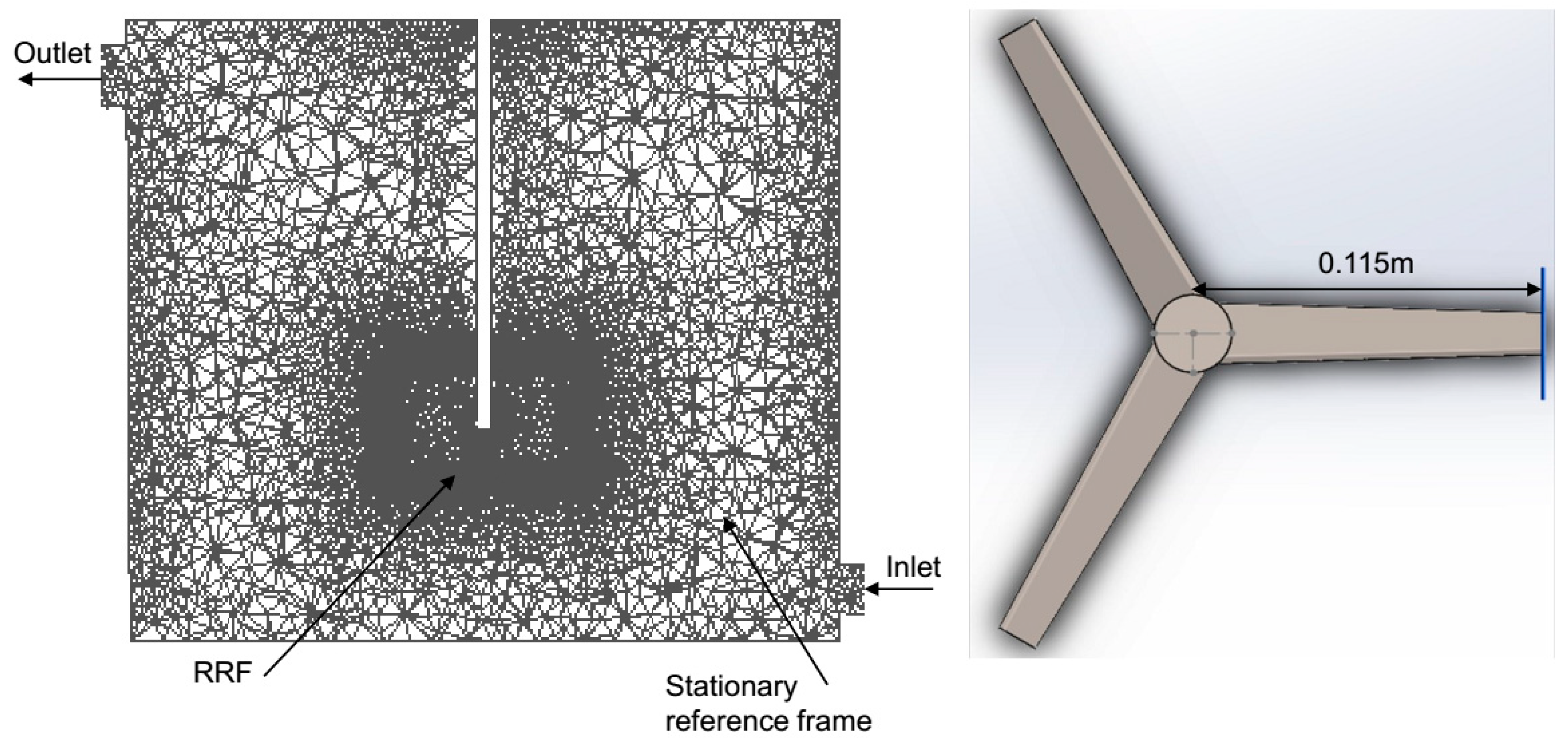
2.1.1. AD Geometry Development and Meshing

The digester with a volume of 1.13 m³ (diameter 1.2 m and height 1 m) and the sludge inside the digester were mechanically agitated by a single-stage mixer with three axial flow hydrofoil impellers (Figure 1, right). The feature of the impeller rotation can be modelled using either the Multiple Reference Frame (MRF) or the sliding mesh approach. Because the sliding mesh approach requires a transient simulation, a very fine mesh for a stable solution, larger computational resources, and a longer simulation time, it was decided to model the flow feature of the AD mixing through the MRF.

The MRF has two flow features: a rotating reference frame (RRF), which encloses the volume surrounding the mixer impellers, and the stationary reference frame. An RRF was connected to the stationary reference frame using an interface boundary condition. The impeller speeds used in the ADs range from low speed to very high speed (up to 800 rpm) depending on the sludge TSS [9,15,24]. We selected an intermediate value of 300 rpm.

Both the stationary and rotating frames of reference were meshed using a tetrahedral mesh with 1.66 million elements (cells) (0.7 mm³/cell) and 0.312 million nodes (Figure 1, left) in which the results are independent of mesh sizes at residual of 10−3. A mesh independent test was analyzed for 95,000 cells, 1.3 million cells, and 1.66 million cells. The percentage error of the velocity distribution between 1.35 and 1.66 million cells is about 5%. Inlet velocity, pressure outlet, and no-slip wall were defined for inlet, outlet, and wall boundary conditions, respectively.

2.1.2. Discretization Method

The SIMPLE (Semi-Implicit Method for Pressure Linked Equations) scheme solver was used for the solution of a steady-state with a k-ε realizable turbulence model. The momentum and turbulent kinetic energy were discretized using a 2nd order upwind scheme while the turbulence dissipation was discretized using a 1st order upwind scheme since it oscillates and does not converge when using a 2nd order upwind scheme.

Continuity and momentum equations of an RRF for absolute velocity formulation are given in Equations (1) and (2), respectively.

$$\nabla .\rho {\overrightarrow{v}}_r=0$$

(1)

$$\nabla .\left(\rho {\overrightarrow{v}}_r\overrightarrow{v}\right)+\rho \left(\overrightarrow{\omega }\times \overrightarrow{v}\right)=-\nabla p+\nabla {\stackrel{=}{\tau }}_r+\overrightarrow{F}$$

(2)

where ${\overrightarrow{v}}_r$ is the relative velocity (the velocity observed from the rotating frame (m/s)), $\overrightarrow{\omega }$ is the angular velocity (1/s), and $\overrightarrow{v}$ is the absolute velocity viewed from the stationary reference frame (m/s).

The realizable turbulence kinetic energy (k) and dissipation rate (ε) were selected based on the work of Wu [25] and given by Equations (3) and (4), respectively.

$$\frac{\partial }{\partial x_i}\left(\rho k{u}_i\right)=\frac{\partial }{\partial x_i}\left[\left(\mu +\frac{{\mu }_t}{{\sigma }_k}\right)\frac{\partial k}{\partial x_i}\right]+G_k+G_b-\rho \epsilon -Y_M+S_k$$

(3)

$$\frac{\partial }{\partial x_i}\left(\rho \epsilon u_i\right)=\frac{\partial }{\partial x_i}\left[\left(\mu +\frac{{\mu }_t}{{\sigma }_{\epsilon }}\right)\frac{\partial \epsilon }{\partial x_i}\right]+\rho C_{1}S\epsilon -C_2\frac{{\epsilon }^2}{k+\sqrt{v\epsilon }}+C_{1\epsilon }\frac{{\epsilon }^2}{k}{C}_{3\epsilon }{G}_b+S_{\epsilon }$$

(4)

where $C_1=\max \left[0.43,\frac{\eta }{\eta +5}\right]$, $\eta =S\frac{k}{\epsilon },$ $S=\sqrt{2S_{ij}{S}_{ij}}$, $C_{1\epsilon },C_2,{\sigma }_k,{\sigma }_{\epsilon }$ are constants with a value of 1.44, 1.9, 1.0 and 1.2, respectively, $G_k$ is the generation of turbulent kinetic energy due to mean velocity gradients, $G_b$ is the generation of turbulent kinetic energy due to buoyancy, S is the modulus of the strain rate tensor, and ${\mathsf{\mu }}_{\mathrm{t}}$ is eddy viscosity. The detailed explanation of $Y_M,G_k, S \mathrm{and} C_{\mu }$ are found in the ANSYS Theory Guide [26].

The Herschel–Bulkley rheology model was selected because it includes non-zero shear stress (yield stress) even when the strain rate is zero [27]. Hence, Equation (5) is solved when $\dot{\mathsf{\gamma }}>{\dot{\mathsf{\gamma }}}_{\mathrm{c}}$ and Equation (6) is solved when $\dot{\mathsf{\gamma }}<{\dot{\mathsf{\gamma }}}_{\mathrm{c}}$. A non-Newtonian rheology model was activated by the user using the Text User Interface (TUI) in the ANSYS FLUENT console.

$$\mathsf{\eta }=\frac{{\mathsf{\tau }}_{\mathrm{y}}}{{\dot{\mathsf{\gamma }}}_{\mathrm{c}}}+\mathrm{K}{\left(\frac{\dot{\mathsf{\gamma }}}{{\dot{\mathsf{\gamma }}}_{\mathrm{c}}}\right)}^{\mathrm{n}-1}$$

(5)

$$\mathsf{\eta }=\frac{{\mathsf{\tau }}_{\mathrm{y}}\left[2-\frac{\dot{\mathsf{\gamma }}}{{\dot{\mathsf{\gamma }}}_{\mathrm{c}}}\right]}{{\dot{\mathsf{\gamma }}}_{\mathrm{c}}}+\mathrm{K}\left[\left(2-\mathrm{n}\right)+\left(\mathrm{n}-1\right)\frac{\dot{\mathsf{\gamma }}}{{\dot{\mathsf{\gamma }}}_{\mathrm{c}}}\right]$$

(6)

where $\mathsf{\eta }$ is the apparent viscosity (Pa. s), $\dot{\mathsf{\gamma }}$ is the shear rate (1/s), $\mathrm{K}$ is the consistency index, n is the flow index, and ${\dot{\mathsf{\gamma }}}_{\mathrm{c}}$ is the critical shear rate. The critical shear rate was added to avoid discontinuity (infinite apparent viscosity) at a very low shear rate [26,27]. K is the consistency index (Pa.sn), n is the power-law index and ${\mathsf{\tau }}_{\mathrm{y}}$ is the yield stress (Pa). The values of K, n and ${\mathsf{\tau }}_{\mathrm{y}}$ were correlated based on the work of Eshtiaghi et al. [28] and Slatter [29] and are shown in

Table 1. The values of consistency index (K), yield stress (${\mathsf{\tau }}_{\mathrm{y}}$) and power-law index (n)

TSS (%)	K	${\mathsf{\tau }}_{\mathbf{y}}$	n
4%	0.02	2.23	0.57
8%	0.16	19.89	0.51
12%	88.44	75.92	0.34

. The effect of sludge rheology was modelled by treating the sludge as a Newtonian fluid (water) for sludge with TSS less than 4% and non-Newtonian fluid with the TSS at 4%, 8%, and 12%.

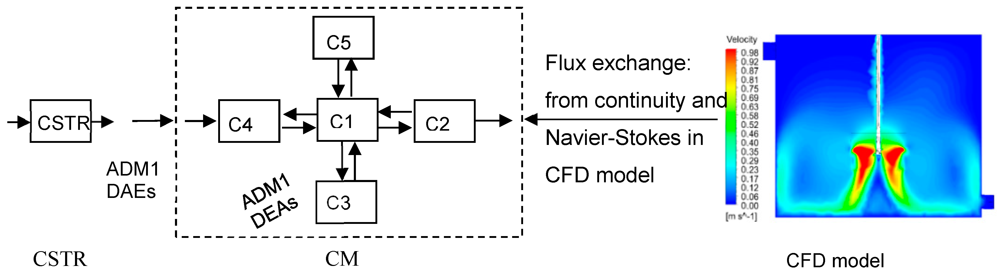
2.2. Compartmentalization of AD from the CFD Model

A CM is a general method of dividing a reactor volume (here an AD) into sub-volumes based on the CFD model velocity distribution to mimic the non-ideal mixing kinetics model. Different methods of compartmentalization have been discussed in the literature, depending on the type of problem. For example, velocity, species concentration, turbulence, and temperature can be applied to compartmentalize the system under study [22] using either manual [20,30] or automatic zoning [31] of the system under study. Due to its flexibility, simplicity, and the fact that the user can decide the number of compartments, the digester was compartmentalized manually based on the velocity distribution in this work.

Figure 2 shows a method of deriving the CM from a CFD hydrodynamic model and links it to AD kinetics. The compartments are linked together by the flux exchange arrows.

The exchange flux between each compartment depends on the local velocity magnitude and the compartment surface area (Equation (7)).

$$q_{exch}=u_{avg}{A}_{surf}$$

(7)

where $u_{avg}$ is the average velocity (m/s) in/out of the compartment and $A_{\mathit{surf}}$ is the surface area of the compartment (m²).

In a CM, each compartment is assumed to be ideally mixed, and as having virtually independent digesters; hence, the ADM1 is implemented in each compartment.

2.3. Implementation of ADM1 into the CM

The steady-state mass balance of the ADM1 soluble substrates and biomass are given in Equations (8) and (9) [1].

$$\frac{{{\displaystyle \sum }}_1^k\left({\mathrm{q}}_{\mathrm{in},\mathrm{k}}{\mathrm{S}}_{\mathrm{in},\mathrm{k}}\right)}{{\mathrm{V}}_{\mathrm{liq}}}-\frac{{\mathrm{q}}_{\mathrm{out}}{\mathrm{S}}_{\mathrm{liq},\mathrm{i}}}{{\mathrm{V}}_{\mathrm{liq}}}+{{\displaystyle \sum }}_{\mathrm{j}=1-19}{\rho }_j{v}_{i,j}=0$$

(8)

$$\frac{{{\displaystyle \sum }}_1^k\left({\mathrm{q}}_{\mathrm{in},\mathrm{k}}{\mathrm{X}}_{\mathrm{in},\mathrm{k}}\right)}{{\mathrm{V}}_{\mathrm{liq}}}-\frac{{\mathrm{q}}_{\mathrm{out}}{\mathrm{X}}_{\mathrm{liq},\mathrm{i}}}{{\mathrm{V}}_{\mathrm{liq}}}+{{\displaystyle \sum }}_{\mathrm{j}=1-19}{\rho }_j{v}_{i,j}=0$$

(9)

where ${\mathrm{q}}_{\mathrm{in}}$ and ${\mathrm{q}}_{\mathrm{out}}$ are the inflow and outflow rate, respectively, ${\mathrm{S}}_{\mathrm{liq}}$ represents the soluble substrates, ${\mathrm{X}}_{\mathrm{liq}}$ represents the biomass fractions, ${\mathrm{V}}_{\mathrm{liq}}$ is the digester liquid volume, ${\rho }_j$ is the uptake rate of process $j$, ${\mathrm{v}}_{\mathrm{i},\mathrm{j}}$ represents the rate coefficients for component i taking part in process $j$, $i$ represents the index soluble substrates and biomass index, and $k$ represents the number inflow rates into the compartment. Since there might be more than one inflow rate into a compartment, the total inflow rate is indicated as the sum of inflow rates.

The biogas flow rate ($q_{gas})$ from each compartment at atmospheric pressure was calculated using Equation (10).

$$q_{gas}=k_p\left(P_{gas}-P_{atm}\right)\frac{P_{gas}}{P_{atm}}$$

(10)

where $k_p$ is related to the biogas outlet friction factor with 5 × 104 m³ d − 1 bar − 1 and $P_{gas}$ is the sum of the partial pressure of methane, CO_2, and water vapor, and P_atm is the atmospheric pressure.

The CM shown in Figure 3 was implemented in WEST software (powered by DHI, Denmark) after extensive customization of the software to fit the modelling goal. The ADM1 model parameter values were taken as proposed in the Benchmark Simulation Model 2 (BSM2) framework [32]. The ADM1 input data were fractionated from chemical oxygen demand (COD), Total kjeldahl Nitrogen (TKN, total suspended solids (TSS), and inflow rate, according to Nopens et al. [33]. The input values of COD, TKN, TSS, and inflow rate were 66 g/L, 0.8 g/L, 47 g/L, and 75 L/d, respectively.

3. Results and Discussion

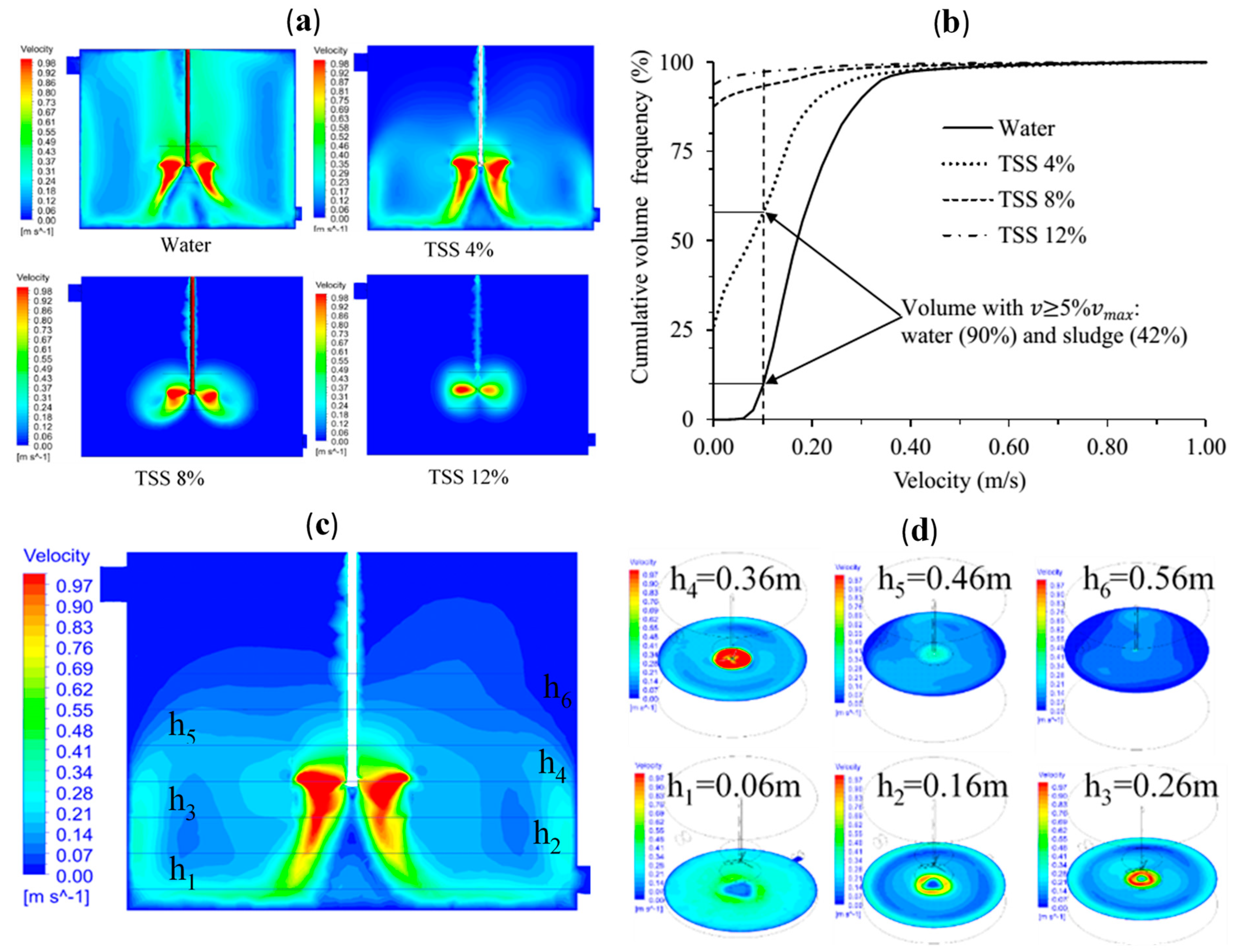
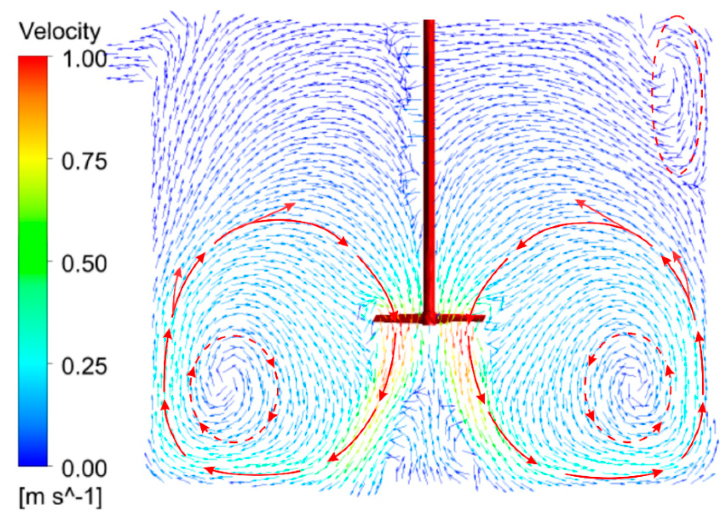
3.1. CFD Model Simulation

The steady-state simulation results of the AD mixing treating the sludge as Newtonian and non-Newtonian fluid are shown in Figure 3a in a vertical plane view. The observation from Figure 3a indicates that the velocity distribution has a good uniformity for Newtonian fluid (water), and the uniformity decreases sharply for non-Newtonian fluid as the sludge TSS increases. At an elevated TSS value, only the sludge near the impeller is moving due to a higher sludge viscosity. This results in a poor velocity distribution (Figure 3) in a similar fashion reported by [9].

Since the contour plot is a qualitative observation and only allows for observation in a plane view in 2-D, quantitative velocity distribution in 3-D is necessary for detailed information on the uniformity of velocity distribution. Quantitative velocity distribution in 3-D is plotted using the cumulative volume frequency of velocity shown in Figure 3b for Newtonian and non-Newtonian fluid.

The maximum velocity near the impeller speed is 2.3 m/s; however, the volume of the sludge, which moves above 1 m/s is minimal and cannot be observed in the cumulative volume frequency of velocity distribution analysis and contour plot. Based on the assumption stated in [9], the digester zone moving at a velocity of less than 5% of the maximum velocity is considered as a stagnant zone. Hence, 10%, 58%, 93%, and 97% of the digester volume has a velocity of less than 5% of the maximum velocity for water and sludge with the TSS at 4%, 8%, and 12%, respectively.

In addition to the vertical plane velocity contour plot and cumulative volume frequency of velocity, the velocity distribution in a horizontal plane view is plotted at different heights of the digester for the sludge with the TSS at 4% (Figure 3d) at an indicated height in Figure 3c to obtain a precise observation of the velocity distribution together with the contour plot in the vertical plane view (Figure 3a) in zoning the digester.

Figure 3c indicates a velocity contour plot of the sludge with the TSS at 4% and sliced at different heights. Since the impellers are axial flow types, the sludge flows through the impeller, and downward velocity is created as indicated in the velocity vector plot (Figure 4). Then the velocity bounces at the bottom of the digester and creates two ‘U’ shaped patterns (Figure 3c), and the uniform velocity distribution is observed at h₁ (Figure 3d). The magnitude and uniformity of velocity decrease from h₁ to h₅. There is a high velocity around the impellers, medium velocity near the wall, and low velocity between the wall and center of the digester. The reason for such a flow formation is due to the nature of the impeller. From h₅ to the top of the digester, the velocity distribution gradually decreases and becomes stagnant.

The velocity vector shown in Figure 4 indicates two types of recirculation. Solid circular arrows indicate recirculation between the high and medium velocity zones, and flow exchange between the zone and its neighborhood exists. In contrast, the dashed arrows indicate the recirculation, which creates a closed-loop. The sludge inside this loop recirculates continuously over an extended time because the exchange flow with its neighborhood is limited. A low-velocity recirculation is also observed in the top right side of the stagnant region.

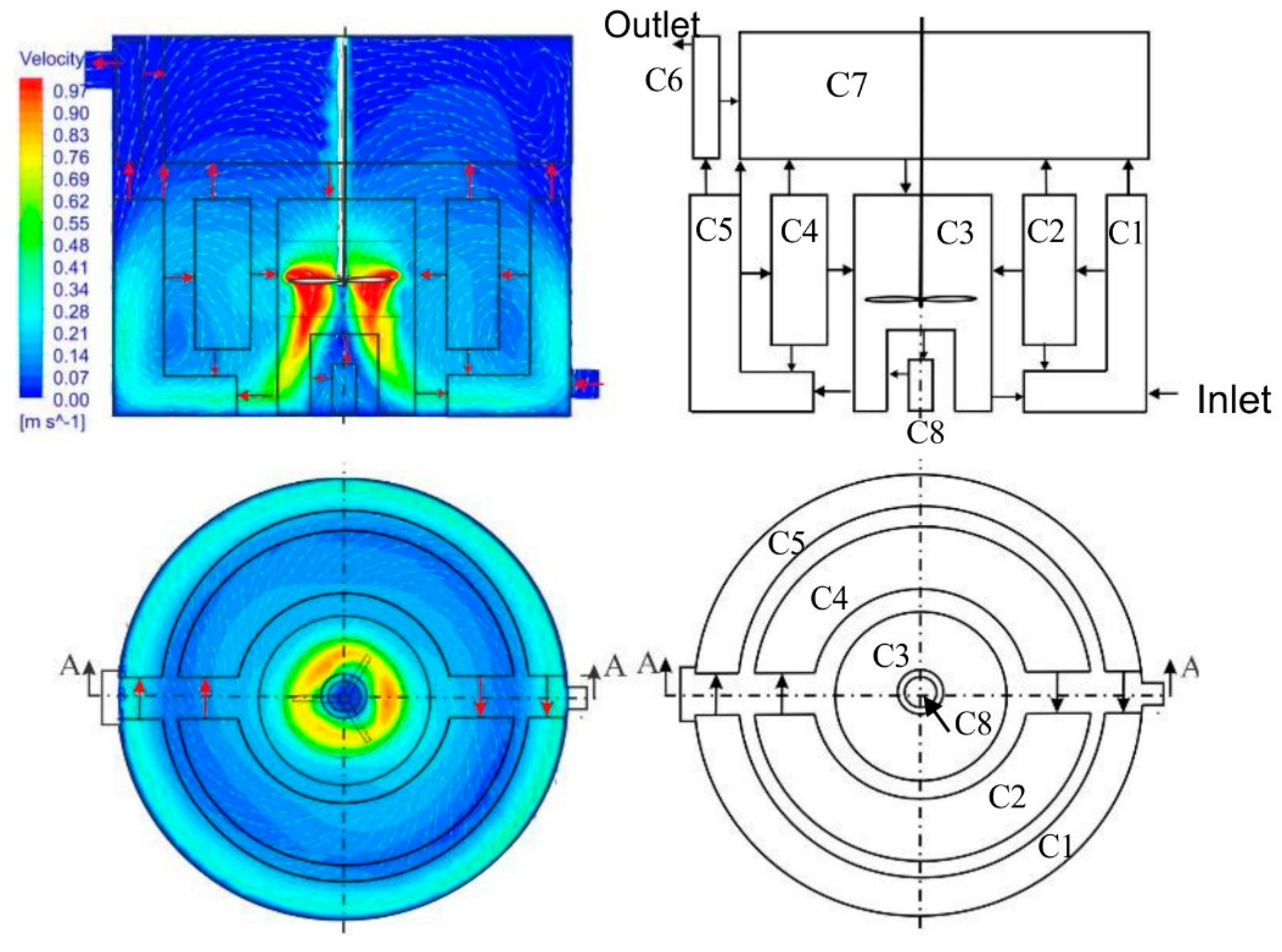
Compartmentalization of AD

The digester is, therefore, categorized into four zones and eight compartments (Figure 5) similar to the work of Le Moullec [20]. The volume of each compartment is calculated from the cumulative volume distribution of velocity shown in Figure 3b.

• Zone one: high-velocity zone (C3). This zone is near the impeller with a velocity magnitude $\ge$ 0.6*maximum velocity (${\overrightarrow{\mathrm{v}}}_{\max }$). The local residence time in this zone is very short due to the high flux exchange. ${\overrightarrow{\mathrm{v}}}_{\max }$ is the sludge velocity near the mixer impeller tip.
• Zone two: medium velocity zone. The velocity in this zone ranges between $0.25{\overrightarrow{\mathrm{v}}}_{\max }\le \overrightarrow{\mathrm{v}}<0.6{\overrightarrow{\mathrm{v}}}_{\max }$. This zone is the outermost of the digester volume with a large diameter with low radial velocity; therefore, the recirculation time is longer. Instead of assuming the zone is a single compartment, it is decided to implement two compartments in series (C1 and C5) to make the residence time more realistic.
• Zone three: low-velocity zone. A zone with a velocity magnitude of $0.05{\overrightarrow{\mathrm{v}}}_{\max }\le \overrightarrow{\mathrm{v}}<0.25{\overrightarrow{\mathrm{v}}}_{\max }$. This zone is divided into two compartments in series (C2 and C4), such as zone two.
• Zone four: Stagnant zone. A very low velocity $<0.05{\overrightarrow{\mathrm{v}}}_{\max })$, and it includes C6, C7, and C8.

The CM accuracy increases with a higher number of compartments, and it can be derived by reducing the tolerance of velocity variation. Hence, the user should decide the required number of CM in conjunction with the modelling goal. It should be bear in mind that every additional compartment adds 32 differential-algebraic equations (DAEs) to the model.

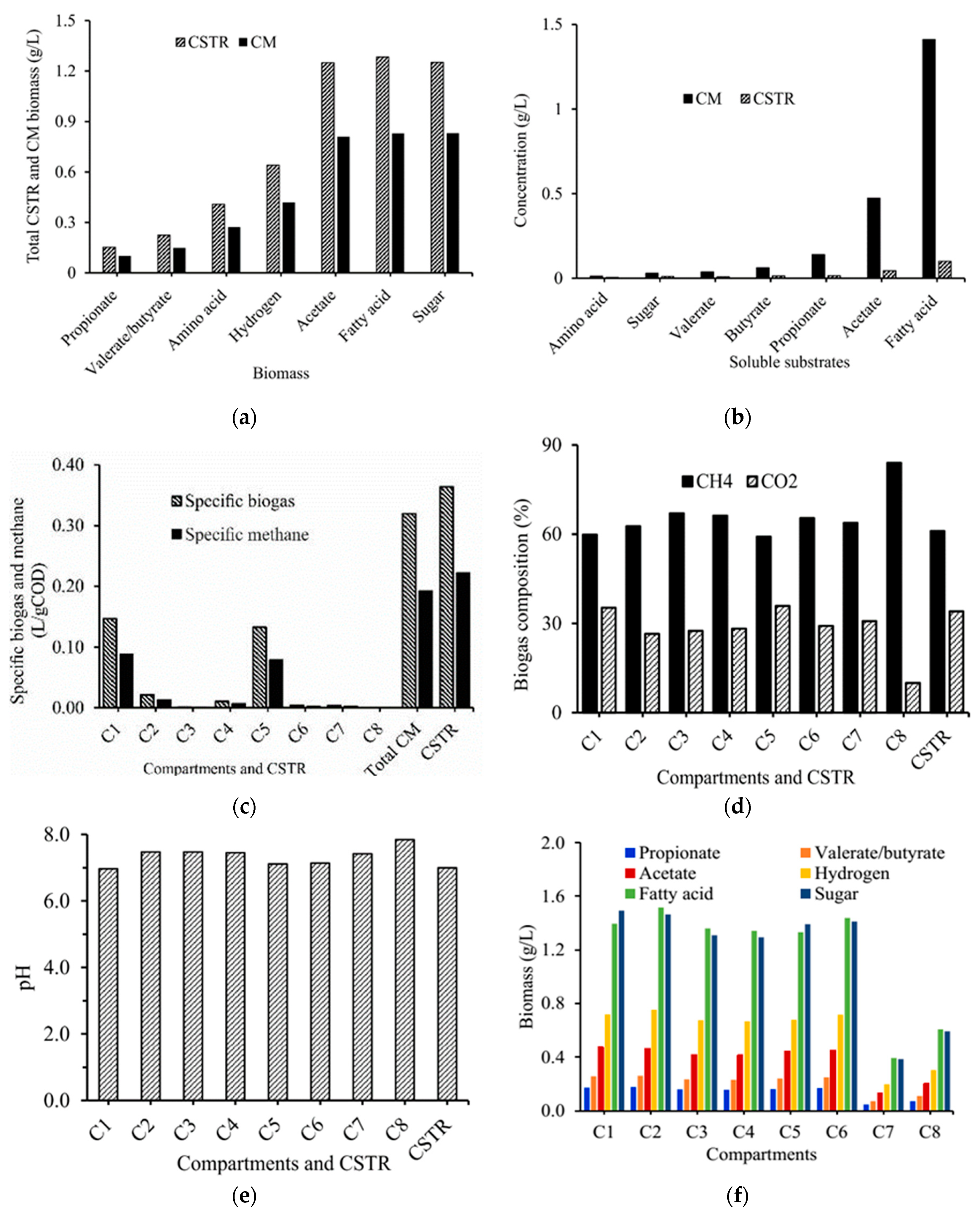
3.2. Non-Ideal Mixing Kinetics Modelling

The spatial variation of biomass, soluble substrates, pH, specific biogas, and methane production in the CM is discussed below and compared with the CSTR AD of the same volume. Figure 6a shows that the biomass concentration in the CM is 35% less than the corresponding CSTR AD. The reduction in hydraulic retention time (HRT) due to the stagnant zone in the CM affects the growth of biomass; hence, it affects the uptake of soluble substrates and reduces the digester performance. The reduction in the biomass concentration in a CM and the stagnant volume (58% of digester volume) are not linearly proportional because a limited amount of biomass grows in the stagnant zones.

The growth of acetogenic biomass (converting volatile fatty acids to acetate) and methanogenic biomass (converting acetate into biogas) are the two most affected in the CM (Figure 6b). The spatial variation of biomass, soluble substrates, pH, specific biogas, and methane production in the CM is discussed below and compared with the CSTR AD of the same volume. Due to the lower biomass growth in the CM (Figure 6a), the undigested soluble substrates outflow from the digester is higher compared to the CSTR digester. The undigested outflow of the soluble acetate and LCFA is 0.4 g/L and 1.4 g/L, respectively, in the CM compared to only 0.04 g/L and 0.1 g/L in the CSTR AD. Moreover, the specific biogas and methane production are reduced by 14% and 16%, respectively, in the CM compared to the CSTR of the same volume (Figure 6c).

The spatial variation of specific biogas and methane in a CM indicates that all zones of the digester are not equally productive in terms of biogas and methane production. About 88% of specific biogas and methane are produced in zone 2 (C1 and C5), which accounts for only 21% of the digester volume (Figure 6c). The reason that most of the biogas is produced in zone 2 can be better understood by observing the CFD model velocity contour (Figure 3) and vectors (Figure 4). The sludge enters zone 2, the outermost compartment (Figure 5) with a larger diameter and medium velocity; this allows the sludge to spend a longer time in zone 2 and so it is digested before entering the adjacent zones. The outflow sludge from zone 2 (inflow into the remaining zones) contains few undigested substrates. Hence the specific biogas and methane production are very low in the remaining zones (Figure 6b). The specific biogas and methane production is reduced by 15% in the non-ideal mixing (CM) compared to the ideal mixing AD (CSTR AD), which is mainly caused by the ineffective digester volume and limited flow exchange between compartments.

As seen in Figure 6d, the biogas composition in zone 2 is 60% CH₄, and 35% CO₂, which is similar to several modelled and measured biogas compositions found elsewhere in the literature. In general, the overall biogas composition in the CM and CSTR is not very different. The weighted average of CH₄ and CO₂ composition in the CM is 63% and 31%, respectively, corresponding to 61% and 34% in the CSTR AD.

The pH distribution in the CM ranges between 6.8 to 7.8, while it is 7.0 and constant in the CSTR AD, as indicated in Figure 6e. The pH of zone 2 (C2 and C5), which produces the highest biogas, ranges between 6.8 and 7.2, and this pH range is suitable for the operation of AD. All the remaining zones of the digester pH are greater than 7.2, and it is not a favorable environment for the growth of biomass. The highest pH is 7.8 in the stagnant zone (C8) and is located under the impeller.

Figure 6f indicates the concentration distribution of biomass in the CM. The biomass concentration in each compartment is nearly uniform in the AD zones, with a significant velocity magnitude shown in Figure 3. This indicates that the biomass growth is not affected as long as adequate flow exchange between the compartments is maintained. Conversely, in the stagnant zones (C7 and C8), the sludge velocity is nearly zero, and so is the exchange flow rate between the compartments; hence, the biomass concentration is the lowest due to substrate limitation for biomass growth.

In general, the non-ideal kinetic model using a CFD-based CM gives a broad and detailed understanding of the biochemical conversion process of AD. It can be applied for AD and mixer design optimization in the pilot and full-scale AD in which the experimental measurement of biochemical reactions is challenging, and hence the challenges of assuming the digester as a CSTR digester can be detached.

4. Conclusions

Knowledge-based derivation of the CM and its implementation developed in this work overcomes the assumption of treating the digester in a CSTR. The model gives the detailed local spatial variation of biochemical processes and resolves the limitations of the CSTR digester, having lower computational requirements and taking a shorter time. The findings of this study showed that all digester volumes are not equally important in biogas production as assumed in a CSTR AD, and the performance is reduced by 15% due to the ineffective use of the digester volume. In addition to predicting the non-ideal biogas and methane production, the CM allows the study of the local kinetic behaviors and factors that affect the AD operation, such as pH, which cannot be studied in a simple model such as CSTR. Furthermore, understanding local biokinetic processes using a CFD-based CM leads to the knowledge-based design of AD for better performance, overcoming the effect of non-ideal mixing and reduction in biogas production. Moreover, a CM model removes the challenges of kinetic model stiffness and huge computational demands encountered in integrating the AD kinetics model into the CFD model.

References

- Batstone, D.; Keller, J.; Angelidaki, I.; Kalyuzhnyi, S.; Pavlostathis, S.; Rozzi, A.; Sanders, W.; Siegrist, H.; Vavilin, V. The IWA Anaerobic Digestion Model No 1 (ADM1). Water Sci. Technol. 2002, 45, 65–73. [Google Scholar] [CrossRef] [PubMed]
- Polizzi, C.; Alatriste-Mondragón, F.; Munz, G. Modeling the Disintegration Process in Anaerobic Digestion of Tannery Sludge and Fleshing. Front. Environ. Sci. 2017, 5, 1–10. [Google Scholar] [CrossRef]
- Kil, H.; Xi, Y.; Li, D. A new waste characterization method for the anaerobic digestion based on ADM1. Chem. Eng. Commun. 2017, 204, 1428–1444. [Google Scholar] [CrossRef]
- Poggio, D.; Walker, M.; Nimmo, W.; Ma, L.; Pourkashanian, M. Modelling the anaerobic digestion of solid organic waste—Substrate characterisation method for ADM1 using a combined biochemical and kinetic parameter estimation approach. Waste Manag. 2016, 53, 40–54. [Google Scholar] [CrossRef] [PubMed] [Green Version]
- Donoso-Bravo, A.; Sadino-Riquelme, C.; Gomez, D.; Segura, C.; Valdebenito, E.; Hansen, F. Modelling of an anaerobic plug-flow reactor. Process analysis and evaluation approaches with non-ideal mixing considerations. Bioresour. Technol. 2018, 260, 95–104. [Google Scholar] [CrossRef] [PubMed]
- Conti, F.; Wiedemann, L.; Sonnleitner, M.; Saidi, A.; Goldbrunner, M. Monitoring the mixing of an artificial model substrate in a scale-down laboratory digester. Renew. Energy 2019, 132, 351–362. [Google Scholar] [CrossRef]
- Wiedemann, L.; Conti, F.; Saidi, A.; Sonnleitner, M.; Goldbrunner, M. Modeling Mixing in Anaerobic Digesters with Computational Fluid Dynamics Validated by Experiments. Chem. Eng. Technol. 2018, 41, 2101–2110. [Google Scholar] [CrossRef]
- Cortada-Garcia, M.; Dore, V.; Mazzei, L.; Angeli, P. Experimental and CFD studies of power consumption in the agitation of highly viscous shear thinning fluids. Chem. Eng. Res. Des. 2017, 119, 171–182. [Google Scholar] [CrossRef]
- Bridgeman, J. Computational fluid dynamics modelling of sewage sludge mixing in an anaerobic digester. Adv. Eng. Softw. 2012, 44, 54–62. [Google Scholar] [CrossRef]
- Yu, L.; Ma, J.; Chen, S. Numerical simulation of mechanical mixing in high solid anaerobic digester. Bioresour. Technol. 2011, 102, 1012–1018. [Google Scholar] [CrossRef]
- Wu, B. Computational Fluid Dynamics Investigation of Turbulence Models for Non-Newtonian Fluid Flow in Anaerobic Digesters. Environ. Sci. Technol. 2010, 44, 8989–8995. [Google Scholar] [CrossRef] [PubMed]
- Wu, B. Integration of mixing, heat transfer, and biochemical reaction kinetics in anaerobic methane fermentation. Biotechnol. Bioeng. 2012, 109, 2864–2874. [Google Scholar] [CrossRef] [PubMed]
- Rezavand, M.; Winkler, D.; Sappl, J.; Seiler, L.; Meister, M.; Rauch, W. A fully Lagrangian computational model for the integration of mixing and biochemical reactions in anaerobic digestion. Comput. Fluids 2019, 181, 224–235. [Google Scholar] [CrossRef]
- Gaden, D.L.F.; Bibeau, E.L. A general three-dimensional extension to ADM1: The importance of an integrated fluid flow model. In Proceedings of the IWA/WEF Wastewater Treatment Seminar, San Francisco, CA, USA, 3–8 November 2013; Volume 4, pp. 318–321. [Google Scholar]
- Delafosse, A.; Collignon, M.-L.; Calvo, S.; Delvigne, F.; Crine, M.; Thonart, P.; Toye, D. CFD-based compartment model for description of mixing in bioreactors. Chem. Eng. Sci. 2014, 106, 76–85. [Google Scholar] [CrossRef]
- Delafosse, A.; Delvigne, F.; Collignon, M.L.; Crine, M.; Thonart, P.; Toye, D. Development of a compartment model based on CFD simulations for description of mixing in bioreactors. Biotechnol. Agron. Soc. Environ. 2010, 14, 517–522. [Google Scholar]
- Gresch, M.; Brügger, R.; Meyer, A.; Gujer, W. Compartmental models for continuous flow reactors derived from CFD simulations. Environ. Sci. Technol. 2009, 43, 2381–2387. [Google Scholar] [CrossRef]
- Wells, G.J.; Ray, W.H. Methodology for modeling detailed imperfect mixing effects in complex reactors. AIChE J. 2005, 51, 1508–1520. [Google Scholar] [CrossRef]
- Delafosse, A.; Calvo, S.; Collignon, M.-L.; Delvigne, F.; Crine, M.; Toye, D. Euler–Lagrange approach to model heterogeneities in stirred tank bioreactors—Comparison to experimental flow characterization and particle tracking. Chem. Eng. Sci. 2015, 134, 457–466. [Google Scholar] [CrossRef]
- Le Moullec, Y.; Gentric, C.; Potier, O.; Leclerc, J. Comparison of systemic, compartmental and CFD modelling approaches: Application to the simulation of a biological reactor of wastewater treatment. Chem. Eng. Sci. 2010, 65, 343–350. [Google Scholar] [CrossRef]
- Spann, R.; Gernaey, K.V.; Sin, G. A compartment model for risk-based monitoring of lactic acid bacteria cultivations. Biochem. Eng. J. 2019, 151. [Google Scholar] [CrossRef]
- Jourdan, N.; Neveux, T.; Potier, O.; Kanniche, M.; Wicks, J.; Nopens, I.; Rehman, U.; Le Moullec, Y. Compartmental Modelling in chemical engineering: A critical review. Chem. Eng. Sci. 2019, 210, 115196. [Google Scholar] [CrossRef]
- Öner, M.; Bach, C.; Tajsoleiman, T.; Molla, G.S.; Freitag, M.F.; Stocks, S.M.; Abildskov, J.; Krühne, U.; Sin, G. Scale-up Modeling of a Pharmaceutical Crystallization Process via Compartmentalization Approach. Comput. Aided Chem. Eng. 2018, 44, 181–186. [Google Scholar]
- Šafarič, L.; Yekta, S.S.; Ejlertsson, J.; Safari, M.; Najafabadi, H.N.; Karlsson, A.; Ometto, F.; Svensson, B.H.; Björn, A.; Yekta, S.; et al. A Comparative Study of Biogas Reactor Fluid Rheology—Implications for Mixing Profile and Power Demand. Processes 2019, 7, 700. [Google Scholar] [CrossRef] [Green Version]
- Wu, B. CFD investigation of turbulence models for mechanical agitation of non-Newtonian fluids in anaerobic digesters. Water Res. 2011, 45, 2082–2094. [Google Scholar] [CrossRef]
- ANSYS. ANSYS Fluent Theory Guide, 15317; ANSYS: Fort Canonville, PA, USA, 2013. [Google Scholar]
- Craig, K.; Nieuwoudt, M.; Niemand, L. CFD simulation of anaerobic digester with variable sewage sludge rheology. Water Res. 2013, 47, 4485–4497. [Google Scholar] [CrossRef] [PubMed] [Green Version]
- Eshtiaghi, N.; Markis, F.; Yap, S.D.; Baudez, J.-C.; Slatter, P. Rheological characterisation of municipal sludge: A review. Water Res. 2013, 47, 5493–5510. [Google Scholar] [CrossRef] [PubMed]
- Slatter, P.T. The rheological characterisation of sludges. Water Sci. Technol. 1997, 36, 9–18. [Google Scholar] [CrossRef]
- Alvarado, A.; Vedantam, S.; Goethals, P.; Nopens, I. A compartmental model to describe hydraulics in a full-scale waste stabilization pond. Water Res. 2012, 46, 521–530. [Google Scholar] [CrossRef]
- Tajsoleiman, T.; Spann, R.; Bach, C.; Gernaey, K.V.; Gernaey, K.V.; Krühne, U. A CFD based automatic method for compartment model development. Comput. Chem. Eng. 2019, 123, 236–245. [Google Scholar] [CrossRef]
- Rosen, C.; Jeppsson, U. Aspects on ADM1 Implementation within the BSM2 Framework; Tech. Rep.; Lund University: Lund, Sweden, 2006; pp. 1–37. [Google Scholar]
- Nopens, I.; Batstone, D.J.; Copp, J.B.; Jeppsson, U.; Volcke, E.I.; Alex, J.; Vanrolleghem, P. An ASM/ADM model interface for dynamic plant-wide simulation. Water Res. 2009, 43, 1913–1923. [Google Scholar] [CrossRef]