Air-Forced Flow in Proton Exchange Membrane Fuel Cells: Calculation of Fan-Induced Friction in Open-Cathode Conduits with Virtual Roughness


Abstract
1. Introduction
1.1. Colebrook Equation for Pipe Flow Friction
1.2. Modified Colebrook Equation for Flow Friction
2. Proposed Model
- laminar flow that depends both on the Reynolds number and on the geometry of conduits; height and width of the mesh of conduits that forms a mesh of cathodic air channels, and
2.1. Turbulent Flow
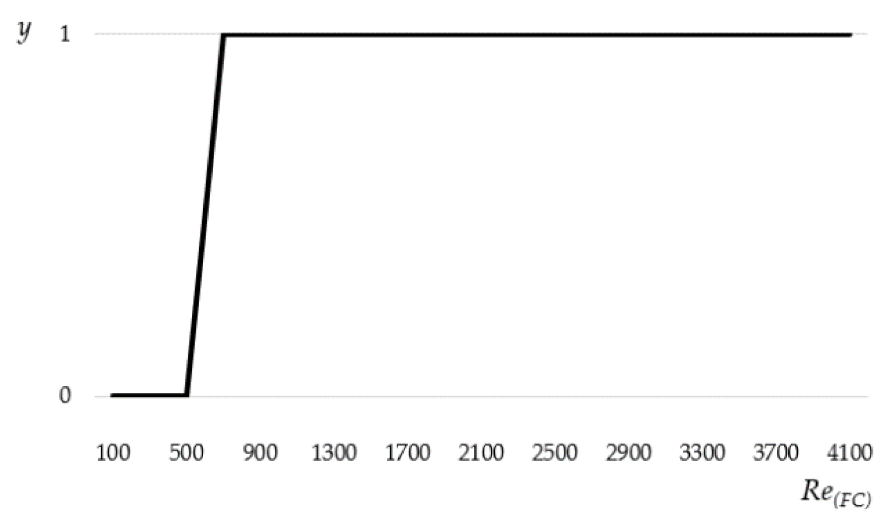
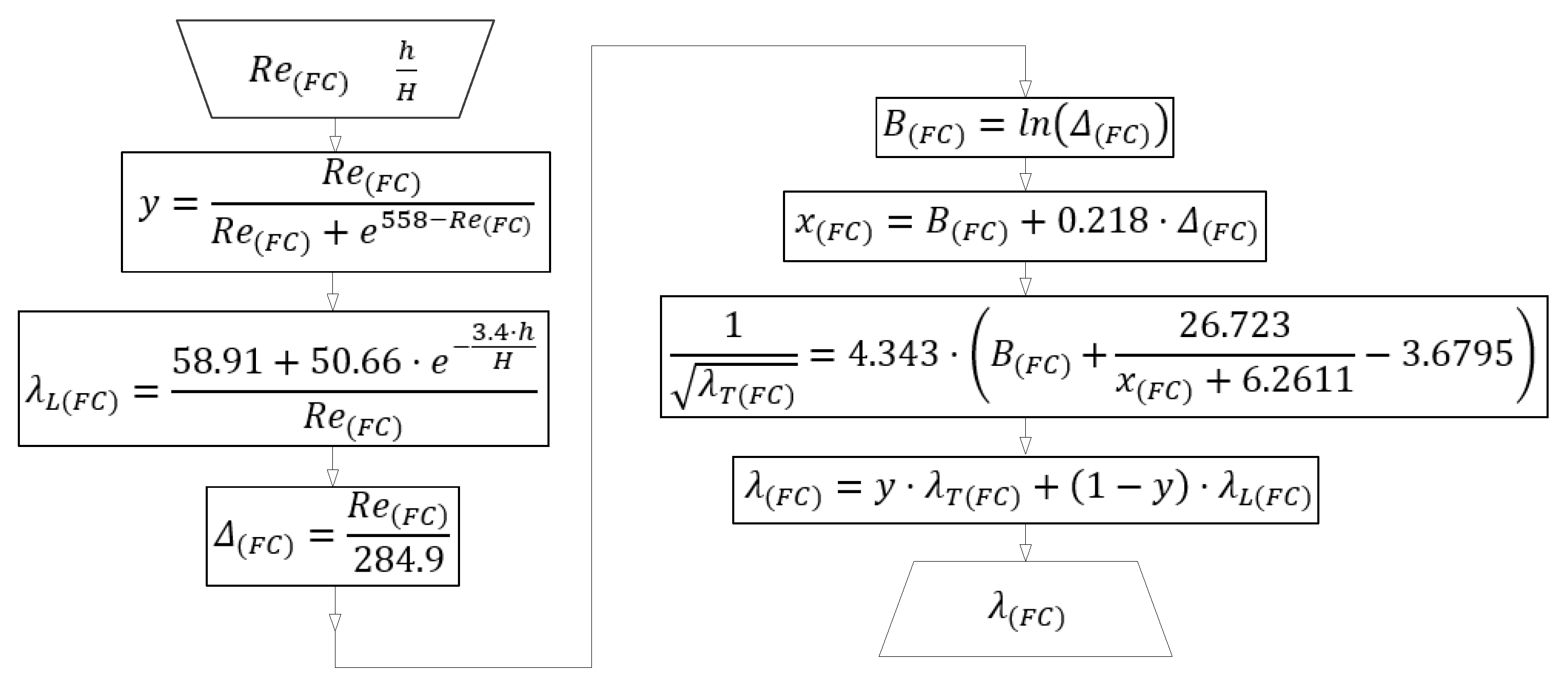
2.2. Unified Model
3. Software Code and Measurement of Execution Speed
4. Conclusions
Author Contributions
Funding
Conflicts of Interest
Notations
| For pipes: | |
| turbulent Darcy flow friction factor for pipes (dimensionless) | |
| turbulent Darcy flow friction factor for pipes (dimensionless) | |
| Reynolds number (dimensionless)—the same definition as for fuel cells | |
| relative roughness of inner pipe surface (dimensionless) | |
| index related to pipes | |
| For Fuel Cells: | |
| unified Darcy flow friction factor for fuel cells (dimensionless) | |
| turbulent Darcy flow friction factor for fuel cells (dimensionless) | |
| laminar Darcy flow friction factor for fuel cells (dimensionless) | |
| Reynolds number (dimensionless)—the same definition as for pipes | |
| virtual relative roughness of fuel cell (dimensionless) | |
| channel depth/channel width used only in laminar flow (dimensionless) | |
| , , | variables |
| , , | constants |
| index related to Fuel Cells | |
| Functions: | |
| logarithmic function with base 10 | |
| natural logarithm | |
| exponential function | |
| Lambert function | |
| Wright function | |
| switching function |
References
- Díaz-Curiel, J.; Miguel, M.J.; Caparrini, N.; Biosca, B.; Arévalo-Lomas, L. Improving basic relationships of pipe hydraulics. Flow Meas. Instrum. 2020, 72, 101698. [Google Scholar] [CrossRef]
- Colebrook, C.F. Turbulent flow in pipes with particular reference to the transition region between the smooth and rough pipe laws. J. Inst. Civ. Eng. 1939, 11, 133–156. [Google Scholar] [CrossRef]
- Colebrook, C.F.; White, C. Experiments with fluid friction in roughened pipes. Proc. R. Soc. Lond. Ser. A Math. Phys. Sci. 1937, 161, 367–381. [Google Scholar] [CrossRef]
- Moody, L.F. Friction factors for pipe flow. Trans. ASME 1944, 66, 671–684. [Google Scholar]
- Hayes, B. Why W? On the Lambert W function, a candidate for a new elementary function in mathematics. Am. Sci. 2005, 93, 104–108. [Google Scholar] [CrossRef]
- Brkić, D.; Praks, P. Accurate and efficient explicit approximations of the Colebrook flow friction equation based on the Wright ω-function. Mathematics 2019, 7, 34. [Google Scholar] [CrossRef]
- Praks, P.; Brkić, D. Review of new flow friction equations: Constructing Colebrook’s explicit correlations accurately. Rev. Int. Métodos Numér. Cálc. Diseño Ing. 2020, 36. in press. [Google Scholar]
- Barreras, F.; López, A.M.; Lozano, A.; Barranco, J.E. Experimental study of the pressure drop in the cathode side of air-forced open-cathode proton exchange membrane fuel cells. Int. J. Hydrogen Energy 2011, 36, 7612–7620. [Google Scholar] [CrossRef]
- Brkić, D. Comments on “Experimental study of the pressure drop in the cathode side of air-forced open-cathode proton exchange membrane fuel cells” by Barreras et al. Int. J. Hydrogen Energy 2012, 37, 10963–10964. [Google Scholar] [CrossRef]
- Smith, R.; Miller, J.; Ferguson, J. Flow of Natural Gas through Experimental Pipelines and Transmission Lines; US Bureau of Mines American Gas Association AGA: New York, NY, USA, 1956; p. 89. [Google Scholar]
- Plascencia, G.; Díaz-Damacillo, L.; Robles-Agudo, M. On the estimation of the friction factor: A review of recent approaches. SN Appl. Sci. 2020, 2, 163. [Google Scholar] [CrossRef]
- Kheirabadi, A.C.; Groulx, D. Cooling of server electronics: A design review of existing technology. Appl. Therm. Eng. 2016, 105, 622–638. [Google Scholar] [CrossRef]
- Khalaj, A.H.; Halgamuge, S.K. A Review on efficient thermal management of air-and liquid-cooled data centers: From chip to the cooling system. Appl. Energy 2017, 205, 1165–1188. [Google Scholar] [CrossRef]
- Soupremanien, U.; Le Person, S.; Favre-Marinet, M.; Bultel, Y. Tools for designing the cooling system of a proton exchange membrane fuel cell. Appl. Therm. Eng. 2012, 40, 161–173. [Google Scholar] [CrossRef]
- Guo, H.; Wang, M.H.; Ye, F.; Ma, C.F. Experimental study of temperature distribution on anodic surface of MEA inside a PEMFC with parallel channels flow bed. Int. J. Hydrogen Energy 2012, 37, 13155–13160. [Google Scholar] [CrossRef]
- Henriques, T.; César, B.; Branco, P.C. Increasing the efficiency of a portable PEM fuel cell by altering the cathode channel geometry: A numerical and experimental study. Appl. Energy 2010, 87, 1400–1409. [Google Scholar] [CrossRef]
- Zhao, C.; Xing, S.; Chen, M.; Liu, W.; Wang, H. Optimal design of cathode flow channel for air-cooled PEMFC with open cathode. Int. J. Hydrogen Energy 2020. [CrossRef]
- Li, C.; Liu, Y.; Xu, B.; Ma, Z. Finite Time thermodynamic optimization of an irreversible Proton Exchange Membrane Fuel Cell for vehicle use. Processes 2019, 7, 419. [Google Scholar] [CrossRef]
- De Lorenzo, G.; Andaloro, L.; Sergi, F.; Napoli, G.; Ferraro, M.; Antonucci, V. Numerical simulation model for the preliminary design of hybrid electric city bus power train with polymer electrolyte fuel cell. Int. J. Hydrogen Energy 2014, 39, 12934–12947. [Google Scholar] [CrossRef]
- Darjat; Sulistyo; Triwiyatno, A.; Sudjadi; Kurniahadi, A. Designing hydrogen and oxygen flow rate control on a solid oxide fuel cell simulator using the fuzzy logic control method. Processes 2020, 8, 154. [Google Scholar] [CrossRef]
- Taner, T. A Flow Channel with Nafion Membrane Material Design of Pem Fuel Cell. J. Therm. Eng. 2019, 5, 456–468. [Google Scholar] [CrossRef]
- Majlan, E.H.; Rohendi, D.; Daud, W.R.W.; Husaini, T.; Haque, M.A. Electrode for proton exchange membrane fuel cells: A review. Renew. Sustain. Energy Rev. 2018, 89, 117–134. [Google Scholar] [CrossRef]
- Fly, A.; Thring, R.H. A comparison of evaporative and liquid cooling methods for fuel cell vehicles. Int. J. Hydrogen Energy 2016, 41, 14217–14229. [Google Scholar] [CrossRef]
- Rahgoshay, S.M.; Ranjbar, A.A.; Ramiar, A.; Alizadeh, E. Thermal investigation of a PEM fuel cell with cooling flow field. Energy 2017, 134, 61–73. [Google Scholar] [CrossRef]
- Topal, H.; Taner, T.; Naqvi, S.A.; Altınsoy, Y.; Amirabedin, E.; Ozkaymak, M. Exergy Analysis of a circulating fluidized bed power plant co-firing with olive pits: A case study of power plant in Turkey. Energy 2017, 140, 40–46. [Google Scholar] [CrossRef]
- Brkić, D. Can pipes be actually really that smooth? Int. J. Refrig. 2012, 35, 209–215. [Google Scholar] [CrossRef]
- Praks, P.; Brkić, D. Choosing the optimal multi-point iterative method for the Colebrook flow friction equation. Processes 2018, 6, 130. [Google Scholar] [CrossRef]
- Praks, P.; Brkić, D. Advanced iterative procedures for solving the implicit Colebrook equation for fluid flow friction. Adv. Civ. Eng. 2018, 2018, 5451034. [Google Scholar] [CrossRef]
- Brkić, D. Review of explicit approximations to the Colebrook relation for flow friction. J. Pet. Sci. Eng. 2011, 77, 34–48. [Google Scholar] [CrossRef]
- Brkić, D.; Praks, P. Unified friction formulation from laminar to fully rough turbulent flow. Appl. Sci. 2018, 8, 2036. [Google Scholar] [CrossRef]
- Barreras, F.; Lozano, A.; Barranco, J.E. Response to the comments on “Experimental study of the pressure drop in the cathode side of air-forced open-cathode proton exchange membrane fuel cells” by Dejan Brkić. Int. J. Hydrogen Energy 2012, 37, 10965. [Google Scholar] [CrossRef][Green Version]
- Sharp, W.W.; Walski, T.M. Predicting internal roughness in water mains. J. AWWA 1988, 80, 34–40. [Google Scholar] [CrossRef]
- Guo, X.; Wang, T.; Yang, K.; Fu, H.; Guo, Y.; Li, J. Estimation of equivalent sand–grain roughness for coated water supply pipes. J. Pipeline Syst. Eng. Pract. 2020, 11, 04019054. [Google Scholar] [CrossRef]
- Bhui, A.S.; Singh, G.; Sidhu, S.S.; Bains, P.S. Experimental investigation of optimal ED machining parameters for Ti-6Al-4V biomaterial. Facta Univ. Ser. Mech. Eng. 2018, 16, 337–345. [Google Scholar] [CrossRef]
- Niazkar, M.; Talebbeydokhti, N.; Afzali, S.H. Novel grain and form roughness estimator scheme incorporating artificial intelligence models. Water Resour. Manag. 2019, 33, 757–773. [Google Scholar] [CrossRef]
- Niazkar, M.; Talebbeydokhti, N.; Afzali, S.H. Development of a new flow-dependent scheme for calculating grain and form roughness coefficients. KSCE J. Civ. Eng. 2019, 23, 2108–2116. [Google Scholar] [CrossRef]
- Andersson, J.; Oliveira, D.R.; Yeginbayeva, I.; Leer-Andersen, M.; Bensow, R.E. Review and comparison of methods to model ship hull roughness. Appl. Ocean Res. 2020, 99, 102119. [Google Scholar] [CrossRef]
- Keady, G. Colebrook-White formula for pipe flows. J. Hydraul. Eng. 1998, 124, 96–97. [Google Scholar] [CrossRef]
- Brkić, D. Lambert W function in hydraulic problems. Math. Balk. 2012, 26, 285–292. Available online: http://www.math.bas.bg/infres/MathBalk/MB-26/MB-26-285-292.pdf (accessed on 21 May 2020).
- Sonnad, J.R.; Goudar, C.T. Constraints for using Lambert W function-based explicit Colebrook–White equation. J. Hydraul. Eng. 2004, 130, 929–931. [Google Scholar] [CrossRef]
- Brkić, D. Comparison of the Lambert W-function based solutions to the Colebrook equation. Eng. Comput. 2012, 29, 617–630. [Google Scholar] [CrossRef]
- Sonnad, J.R.; Goudar, C.T. Turbulent flow friction factor calculation using a mathematically exact alternative to the Colebrook–White equation. J. Hydraul. Eng. 2006, 132, 863–867. [Google Scholar] [CrossRef]
- Biberg, D. Fast and accurate approximations for the Colebrook equation. J. Fluids Eng. Trans. ASME 2017, 139, 031401. [Google Scholar] [CrossRef]
- Muzzo, L.E.; Pinho, D.; Lima, L.E.; Ribeiro, L.F. Accuracy/speed analysis of pipe friction factor correlations. In Proceedings of the International Congress on Engineering and Sustainability in the XXI Century 2019, Faro, Portugal, 9–11 October 2019; pp. 664–679. [Google Scholar] [CrossRef]
- Zeyu, Z.; Junrui, C.; Zhanbin, L.; Zengguang, X.; Peng, L. Approximations of the Darcy–Weisbach friction factor in a vertical pipe with full flow regime. Water Supply 2020. [Google Scholar] [CrossRef]
- Dubčáková, R. Eureqa: Software review. Genet. Program. Evol. M. 2011, 12, 173–178. [Google Scholar] [CrossRef]
- Schmidt, M.; Lipson, H. Distilling free-form natural laws from experimental data. Science 2009, 324, 81–85. [Google Scholar] [CrossRef]
- Wagner, S.; Kronberger, G.; Beham, A.; Kommenda, M.; Scheibenpflug, A.; Pitzer, E.; Vonolfen, S.; Kofler, M.; Winkler, S.; Dorfer, V.; et al. Architecture and design of the HeuristicLab optimization environment. Top. Intell. Eng. Inform. 2014, 6, 197–261. [Google Scholar] [CrossRef]
- Sobol, I.M.; Turchaninov, V.I.; Levitan, Y.L.; Shukhman, B.V. Quasi-Random Sequence Generators; Distributed by OECD/NEA Data Bank; Keldysh Institute of Applied Mathematics; Russian Academy of Sciences: Moscow, Russia, 1992; Available online: https://ec.europa.eu/jrc/sites/jrcsh/files/LPTAU51.rar (accessed on 20 May 2020).
- Winning, H.K.; Coole, T. Explicit friction factor accuracy and computational efficiency for turbulent flow in pipes. Flow Turbul. Combust. 2013, 90, 1–27. [Google Scholar] [CrossRef]
- Winning, H.K.; Coole, T. Improved method of determining friction factor in pipes. Int. J. Numer. Methods Heat Fluid Flow 2015, 25, 941–949. [Google Scholar] [CrossRef]
- Praks, P.; Brkić, D. Rational Approximation for Solving an Implicitly Given Colebrook Flow Friction Equation. Mathematics 2020, 8, 26. [Google Scholar] [CrossRef]
- Taner, T. Energy and Exergy Analyze of PEM fuel cell: A case study of modeling and simulations. Energy 2018, 143, 284–294. [Google Scholar] [CrossRef]
- Andaloro, L.; Napoli, G.; Sergi, F.; Dispenza, G.; Antonucci, V. Design of a hybrid electric fuel cell power train for an urban bus. Int. J. Hydrogen Energy 2013, 38, 7725–7732. [Google Scholar] [CrossRef]
- Taner, T. Alternative energy of the future: A technical note of PEM fuel cell water management. J. Fundam. Renew. Energy Appl. 2015, 5, 1000163. [Google Scholar]
- Andaloro, L.; Arista, A.; Agnello, G.; Napoli, G.; Sergi, F.; Antonucci, V. Study and design of a hybrid electric vehicle (Lithium Batteries-PEM FC). Int. J. Hydrogen Energy 2017, 42, 3166–3184. [Google Scholar] [CrossRef]
- Taner, T. The micro-scale modeling by experimental study in PEM fuel cell. J. Therm. Eng. 2017, 3, 1515–1526. [Google Scholar] [CrossRef]
- Napoli, G.; Micari, S.; Dispenza, G.; Di Novo, S.; Antonucci, V.; Andaloro, L. Development of a fuel cell hybrid electric powertrain: A real case study on a Minibus application. Int. J. Hydrogen Energy 2017, 42, 28034–28047. [Google Scholar] [CrossRef]
- Taner, T.; Naqvi, S.A.; Ozkaymak, M. Techno-Economic Analysis of a more efficient hydrogen generation system prototype: A case study of PEM electrolyzer with Cr-C coated Ss304 bipolar plates. Fuel Cells 2019, 19, 19–26. [Google Scholar] [CrossRef]
- Mendicino, G.; Colosimo, F. Reply to Comment by J. Qin and T. Wu on “Analysis of flow resistance equations in gravel bed rivers with intermittent regimes: Calabrian fiumare data set”. Water Resour. Res. 2020, 56, e2019WR027003. [Google Scholar] [CrossRef]


© 2020 by the authors. Licensee MDPI, Basel, Switzerland. This article is an open access article distributed under the terms and conditions of the Creative Commons Attribution (CC BY) license (http://creativecommons.org/licenses/by/4.0/).
Share and Cite
Brkić, D.; Praks, P. Air-Forced Flow in Proton Exchange Membrane Fuel Cells: Calculation of Fan-Induced Friction in Open-Cathode Conduits with Virtual Roughness. Processes 2020, 8, 686. https://doi.org/10.3390/pr8060686
Brkić D, Praks P. Air-Forced Flow in Proton Exchange Membrane Fuel Cells: Calculation of Fan-Induced Friction in Open-Cathode Conduits with Virtual Roughness. Processes. 2020; 8(6):686. https://doi.org/10.3390/pr8060686
Chicago/Turabian StyleBrkić, Dejan, and Pavel Praks. 2020. "Air-Forced Flow in Proton Exchange Membrane Fuel Cells: Calculation of Fan-Induced Friction in Open-Cathode Conduits with Virtual Roughness" Processes 8, no. 6: 686. https://doi.org/10.3390/pr8060686
APA StyleBrkić, D., & Praks, P. (2020). Air-Forced Flow in Proton Exchange Membrane Fuel Cells: Calculation of Fan-Induced Friction in Open-Cathode Conduits with Virtual Roughness. Processes, 8(6), 686. https://doi.org/10.3390/pr8060686