Article

Generalization of the FOPDT Model for Identification and Control Purposes

by
Cristina I. Muresan
1 and
Clara M. Ionescu
1,2,3,*
1
Department of Automatic Control, Technical University of Cluj-Napoca, Memorandumului 28, 400114 Cluj, Romania
2
DySC Research Group on Dynamical Systems and Control, Department of Electromechanical, System and Metal Engineering, Ghent University, Tech Lane Science Park 125, B9052 Ghent, Belgium
3
EEDT—Decisions and Control Core Lab Flanders Make, Tech Lane Science Park 131, B9052 Ghent, Belgium
*
Author to whom correspondence should be addressed.
Processes 2020, 8(6), 682; https://doi.org/10.3390/pr8060682
Submission received: 29 April 2020 / Revised: 24 May 2020 / Accepted: 5 June 2020 / Published: 10 June 2020
(This article belongs to the Section Process Control and Monitoring)

Abstract

:
This paper proposes a theoretical framework for generalization of the well established first order plus dead time (FOPDT) model for linear systems. The FOPDT model has been broadly used in practice to capture essential dynamic response of real life processes for the purpose of control design systems. Recently, the model has been revisited towards a generalization of its orders, i.e., non-integer Laplace order and fractional order delay. This paper investigates the stability margins as they vary with each generalization step. The relevance of this generalization has great implications in both the identification of dynamic processes as well as in the controller parameter design of dynamic feedback closed loops. The discussion section addresses in detail each of this aspect and points the reader towards the potential unlocked by this contribution.

1. Introduction

The FOPDT (First Order Plus Dead Time) model is a trademark approximation of process dynamic response for the purpose of control design. In the design of a feedback control loop, one considers its performance to a load disturbance or set-point change, its robustness to the changes in the controlled process characteristics, and its fragility to the variation of its own parameters. Several methods are proposed to tune controllers taking into account these features, while approximating the true process dynamic response with FOPDT [1]. Industry reports that PID-type control (Proportional Integral Derivative) is still the frontline feedback algorithm and that identification is still responsible for large costs [2]. Hence, approximations such as FOPDT are useful to allow first hand control design methods for non-control-expert process operators such as broadly exemplified in [3].
Frequency response based optimal tuning for PID-type controllers is very popular for both classical and fractional order PID-type controllers [4,5,6,7,8,9]. Stability margins are imposed as part of the design, such as gain and phase margin. These are intrinsically used to determine the amount of robustness one aims for the closed loop characteristic behavior. Optimal tuning rules for PID-type control have been broadly analysed in frequency domain [10,11]. Fragility for integer order PID-type control [1] and for fractional order PID-type control [12,13,14] is an important measure to account for robustness to dynamic process variability. Dead time variability is an important factor in determining the amount of fragility of a process, and fractional order control has proven to be intrinsically robust to these variations [15].
In this paper we restrict our attention to the generalization of the classical FOPDT model and the implications thereof with respect to gain and phase margins. The contribution of the work is the full generalization of orders in the FOPDT and the corresponding analysis with perspectives for identification and control opportunities.

2. The Generalization of the FOPDT Model

The classical FOPDT model has the form:
P 1 ( s ) = K T s + 1 e T d s
with K the gain; T the time constant and T d the time delay of the approximated process. This is referred to as the integer FOPDT model.
The first generalization was proposed in [16] as a fractional order transfer function with integer order dead time:
P 2 ( s ) = K T s α + 1 e T d s
with α R . We will refer to this form as FO f PDT.
The second generalization was proposed in [17] as an integer first order transfer function with a fractional order dead time:
P 3 ( s ) = K T s + 1 e T d s β
with β R . We will refer to this form as FOPDT f .
Here, we add the complete generalization, i.e., a fractional order transfer function with fractional order dead time:
P 4 ( s ) = K T s α + 1 e T d s β
with ( α , β ) R . We will refer to this form as FO f PDT f .
When control design is envisaged, the robustness of the closed loop is measured in terms of the stability margins: gain and phase margin. The open loop gain and phase margin are then determined such that the controller parameters compensate towards the desired closed loop values. The phase margin (PM) and gain margin (GM) of the loop transfer function will be used to provide the analysis among the four FOPDT models.
The PM for the classical FOPDT model (1) is given by
P M 1 = arctan ( T ω g ) T d ω g + π
where ω g is the gain cross-over frequency in rad/s. The GM is given by
G M 1 = 1 K e T d j ω p T j ω p + 1 = T j ω p + 1 K = T 2 ω p 2 + 1 K
where j = 1 and ω p the phase cross-over frequency in rad/s.
The PM for the FO f PDT model (2) is given by
P M 2 = arctan T ω g α sin α π 2 T ω g α cos α π 2 + 1 T d ω g + π
and the corresponding GM is given by
G M 2 = T 2 ω p 2 α + 2 T ω p α cos α π 2 + 1 K
The PM for the FOPDT f model (3) is given by
P M 3 = arctan ( T ω g ) T d ω g β sin β π 2 + π
and the GM is given by
G M 3 = 1 K e T d j ω p β T j ω p + 1 = T 2 j ω p 2 + 1 K e T d ω p β cos β π 2
The PM for the FO f PDT f model (4) is given by
P M 4 = arctan T ω g α sin α π 2 T ω g α cos α π 2 + 1 T d ω g β sin β π 2 + π
and the GM is given by
G M 4 = T ( j ω p ) α + 1 K e T d ( j ω p β ) = T 2 ω p 2 α + 2 T ω p α cos α π 2 + 1 K e T d ω p β cos β π 2
respectively.

3. Analysis

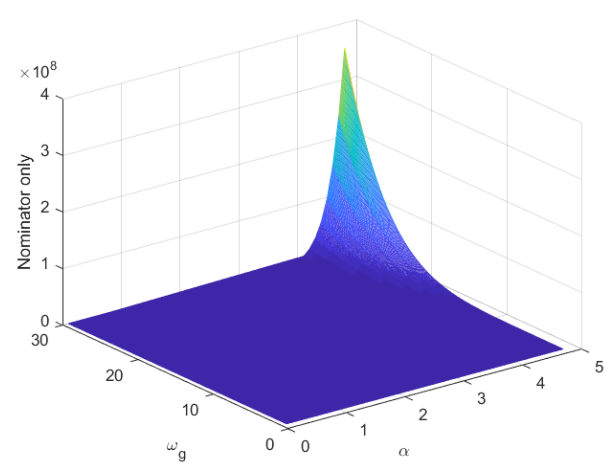
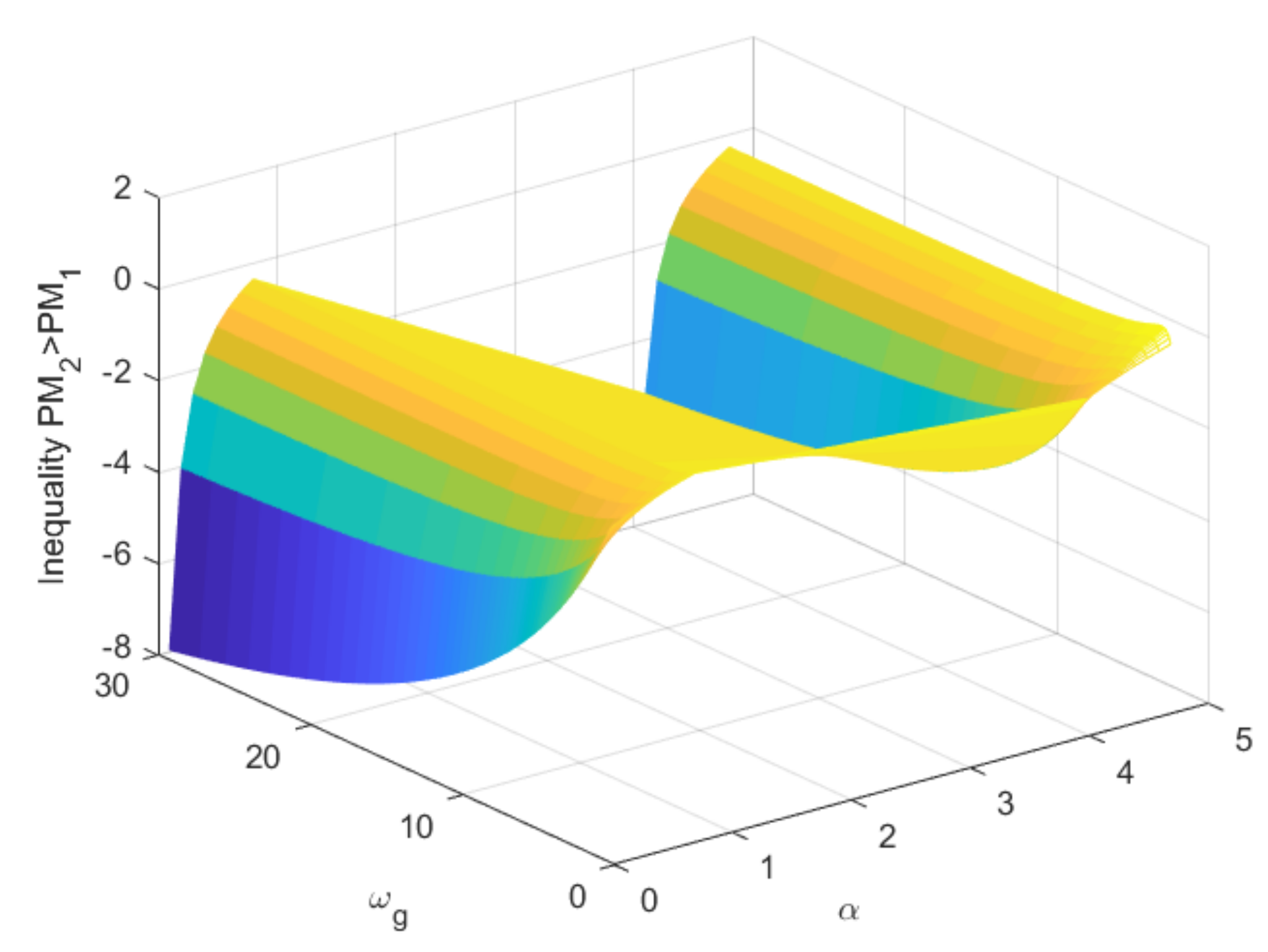
3.1. Effect of Augmentation with Fractional Order Time Constant Term

Let us commence by looking at the system augmented from (1) to (2). The extra parameter is the fractional order α .
Theorem 1.
For any given ω g > 1 and ω p > 1 , there exists an α > 0 R , such that a system augmented with order α has increased robustness.
Proof of Theorem 1.
For the gain margin, assuming that G M 2 G M 1 gives
T 2 ω p 2 α + 2 T ω p α cos α π 2 + 1 K T 2 ω p 2 + 1 K
Simplifying on both sides delivers the inequality
T 2 ( ω p 2 α ω p 2 ) + 2 T ω p α cos α π 2 0
In (14) the first left hand term is always positive for α > 1 , while the term in cosine is periodically positive in intervals α ( 0 , 1 ) ( 3 , 5 ) ( 7 , 9 ) . For all these intervals, the inequality holds, as depicted in Figure 1, available program in Supplementary Material. The same inequality is derived for G M 4 > G M 3 .
Let us now assume that P M 2 P M 1 . We obtain
arctan T ω g α sin α π 2 T ω g α cos α π 2 + 1 arctan ( T ω g )
equivalent to
arctan T ω g α sin α π 2 T ω g α cos α π 2 + 1 T ω g 1 + T ω g α sin α π 2 T ω g α cos α π 2 + 1 T ω g 0
This gives the inequality
T ω g α sin α π 2 T 2 ω g α + 1 cos α π 2 T ω g T ω g α cos α π 2 + T 2 ω g α + 1 sin α π 2 + 1 0
The denominator in (17) is always positive for monotonically increasing values of sin ( α π / 2 ) , that is α ( 0 , 1 ) ( 3 , 5 ) ( 7 , 9 ) . This is illustrated in Figure 2.
For the inequality (17) to hold, we need the sign of the numerator to be negative. For same values of α as above, the numerator is negative. The result is illustrated in Figure 3, available program in Supplementary Material. □
Notice the same inequality is obtained for P M 4 P M 3 .

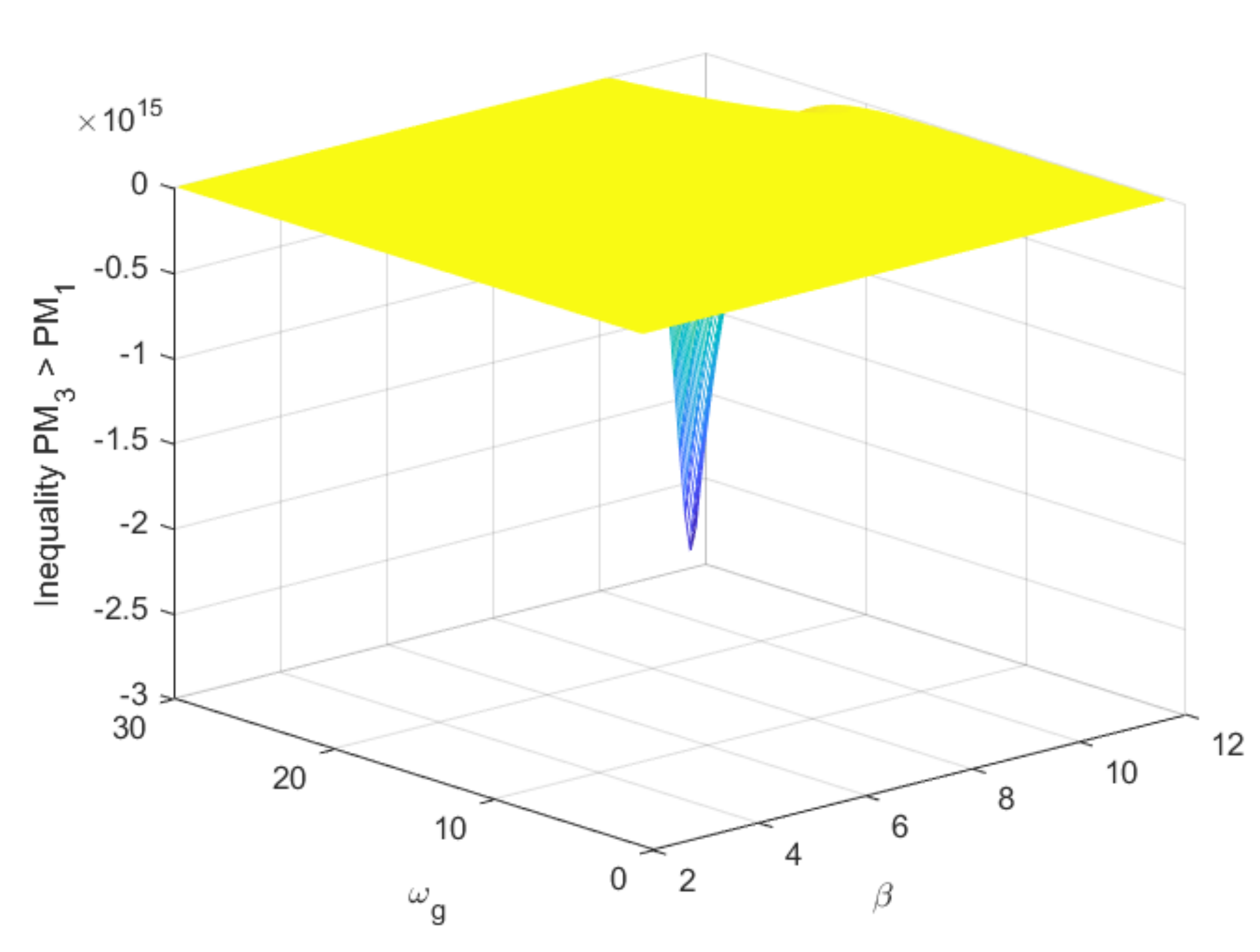
3.2. Effect of Augmentation with Fractional Order Time Delay Term
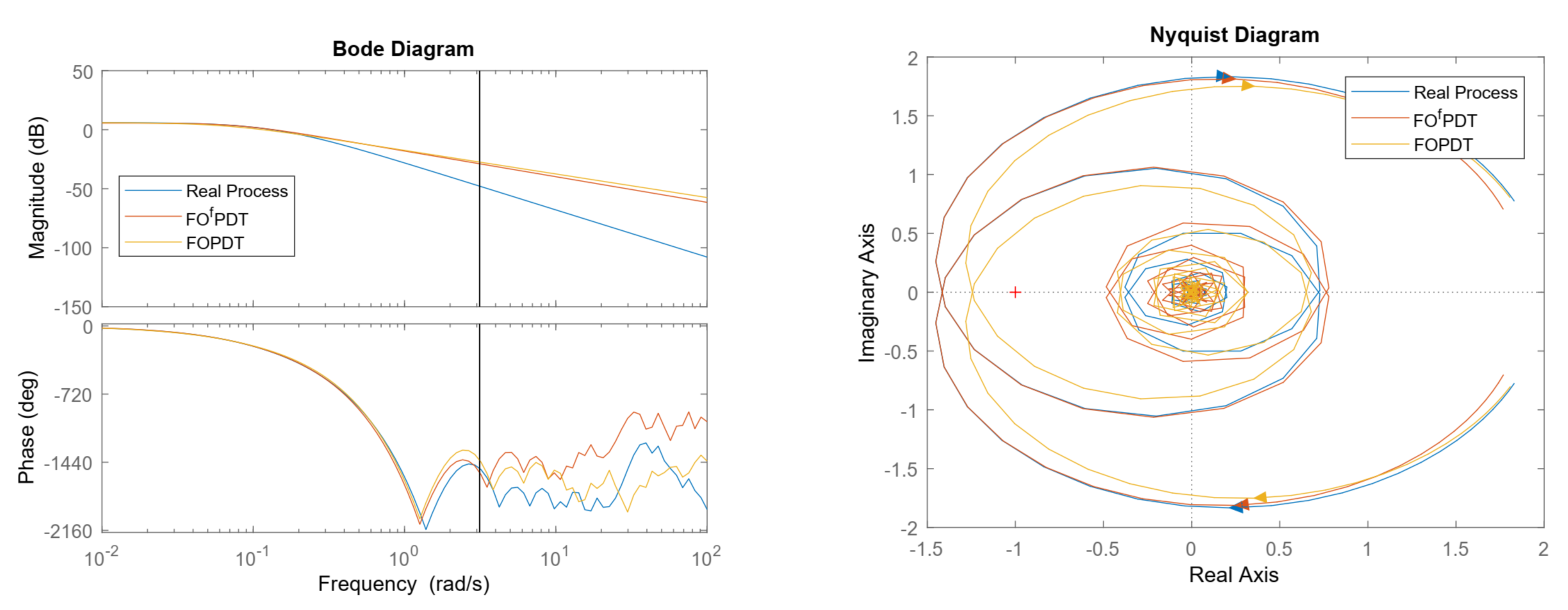
Let us now examine the system augmented from (1) to (3). The extra parameter is the fractional order delay β .
Theorem 2.
For any given ω g > 1 and ω p > 1 , there exists an β > 0 R , such that a system augmented with order β has increased robustness.
Proof of Theorem 2.
Assume G M 3 G M 1 . It follows that
1 e T d ω p β cos β π 2 1
Equivalently,
e T d ω p β cos β π 2 e 0
following that
T d ω p β cos β π 2 0
For T d > 0 and ω p > 0 we have that T d ω p β > 0 and the simplified inequality holds
cos β π 2 0
Inequality (21) holds for values β ( 0 , 1 ) ( 3 , 5 ) ( 7 , 9 ) .
Assume P M 3 P M 1 . It follows that
T d ω g β sin β π 2 T d ω g
with T d > 0 and ω g > 0 . Division with right hand side term gives
ω g β ω g sin β π 2 1
The inequality follows
ω g ( β 1 ) sin β π 2 1 0
This inequality holds for negative values of sinusoidal function, i.e., β ( 2 , 4 ) ( 6 , 8 ) ( 10 , 12 ) . Figure 4 illustrates this result, available program in Supplementary Material.
For both inequalities (21) and (24) simultaneously, then β ( 3 , 4 ) ( 7 , 8 ) . □
The same inequalities are valid for G M 4 > G M 2 and P M 4 > P M 2 .

4. Discussion

4.1. On Identification

By definition, a fractional order derivative s α implies a higher order of equivalent electrical of R-L elements; while a fractional order integrator 1 s β implies a higher order of equivalent electrical R-C elements [18,19]. The frequency intervals where these high order systems are operating are significantly different, i.e., higher vs lower frequency bandwidth. This influences also the achievable closed loop bandwidth.
Typical processes where setpoint tracking is envisaged will abide to lower frequency bands, while processes where essentially disturbance rejection mode is used will abide to band-limited intervals. Finally, stochastic noise will be visible at higher frequencies. Control theory has shown that no single controller can adequately handle all above mentioned modes of operation, unless detuned for high robustness over a large frequency interval of operation [11,20]. In practice, separate controllers (feedback, feedforward, lead-lag, lag-lead etc) will be used to tackle the various frequency intervals of interest.
Figure 5 presents the four model structures by means of Nyquist plot frequency response for various values of their fractional orders. It can be observed the difference in frequency intervals where the fractional order affects the frequency response. Figures also available via program in Supplementary Material.
In our prior work described in [16], we presented generic LTI (linear time invariant) systems to describe transfer functions of incommensurate real orders involving fractional order time constant terms. Process model given by (2) has been used to identify the process dynamic response from a simple sinusoidal experiment. The identification procedure has been successfully applied both in simulation and in experimental data and has been used for both in system identification [16] as well as in controller tuning [7].
It has been shown in [16] that such a FO f PDT model has the least number of unknown parameters compared to real process high order dynamics. The ability to capture effortlessly the high order dynamics is in the geometrical meaning of the fractional order, related to the frequency response of the system. One such fractional order value is equivalent to an interlacing of pole-zero pairs in a band-limited interval.
The conditions for robustness analyzed in the previous section can be thus used to pose restrictions in the identification domain of solutions. This is directly applicable with the identification method described in [16], as the coefficient α is preset in a user-determined interval to speed up the convergence of the identification procedure.
The process model from (3) has been identified from an experimental circuit of RC elements in a ladder network configuration [17]. The fractional order delay coefficient has been shown to improve the fitting in frequency domain for faster decay of phase at higher frequencies. This high frequency behavior is also observed in delay–dominant systems. It has been observed that increasing the delay coefficient value results in decreasing the fractional order delay coefficient value. However, in the classical β = 1 form such as in (1), increasing the delay coefficient value alone exhibited poor fitting performance.
A summary of the real life processes where some of these structures are used, is given in Table 1. Variations of fractional order model (with/-out time delay in model structure) with multiple fractional order time constants have been omitted from the list, but real life examples are numerous and in various application areas; see e.g. numerous works involving experimental data based identification of fractional order dynamic systems of J.A. Tenreiro Machado, R. Caponetto and H. HosseinNia.

4.1.1. Identification Procedure
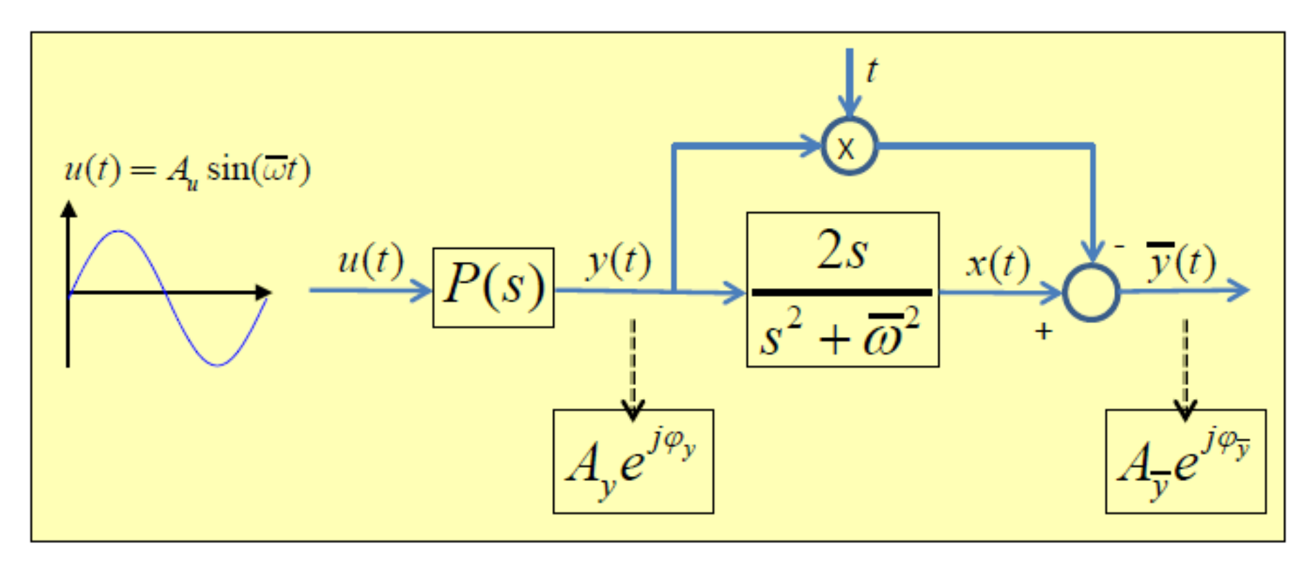
There exist identification procedures for FOPDT and SOPDT (Second Order Plus Dead Time) model approximations from real data [16,26,27]. Here we give a summary of the employed method used in this paper in the two numerical examples given hereafter. In Appendix A we give a summary of the estimation method from [16] for the FOPDT and FO f PDT model structures. The identification method used in [17] for the FOPDT f model structure is based on nonlinear least squares identification method from experimental multisine data, without specific considerations on the fractional order interval values. Any other optimization method can be used to extract/identify the model parameters from experimental data.
  • Select a test frequency ω ¯ . As mentioned in [7,16], the critical frequency (i.e., phase crossover frequency) is a suitable candidate.
  • Do a sine test with ω ¯ using the scheme in Figure 6. The process frequency response P ( j ω ¯ ) and its slope d P ( j ω ) d ω ω ¯ can be obtained from the magnitude and phase of the signals y ( t ) and y ¯ ( t ) . In Figure 6, P ( s ) represents the real physical process and y ( t ) represents the measured process output. The underlying theory has been described in [28] and the method validated as robust against process disturbances and measurement noise.
  • Obtain a simple FO f PDT model of the physical process with the method described in [16].
  • Convert the FO f PDT model into a discrete-time transfer function for digital control purposes. A procedure to convert any fractional order model into a discrete-time transfer function has been described in [29].

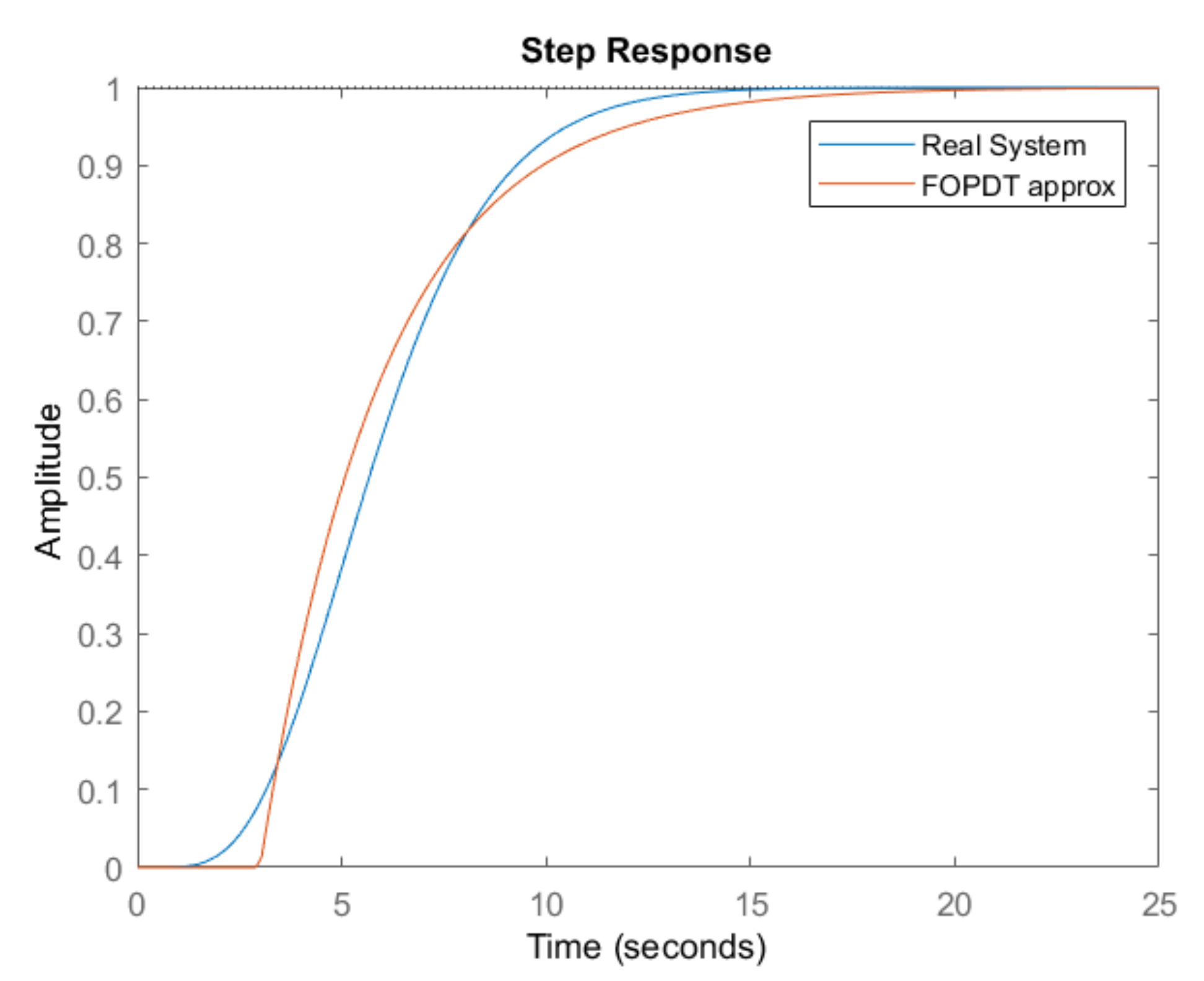
4.1.2. High Order Process Example

Let us consider the high order process model example from [16]:
P ( s ) = 1 ( s + 1 ) 6
with sampling period T s = 0.3 and the FOPDT approximation given by
P a p ( s ) = 1 ( 3 s + 1 ) e 3 s
The step response is given in Figure 7. Notice that in practice, the FOPDT approximation is done by trial-and-error manner, and the result is quite good. However, the S-shape of the high order system is clearly far from being adequately captured by the first order dynamic characteristic.
The identified FO f PDT model has the form
P i d ( s ) = 0.8983 3.6223 s 1.161 + 1 e 3.0259 s
where no constraints have been put on the values of α . The stability margins are given in Table 2 below and the frequency response in terms of Bode and Nyquist plots in Figure 8, available with program in Supplementary Material. Notice in the Nyquist diagram a distinct ability of the identified FO f PDT model to outperform the FOPDT in terms of curve fitting.

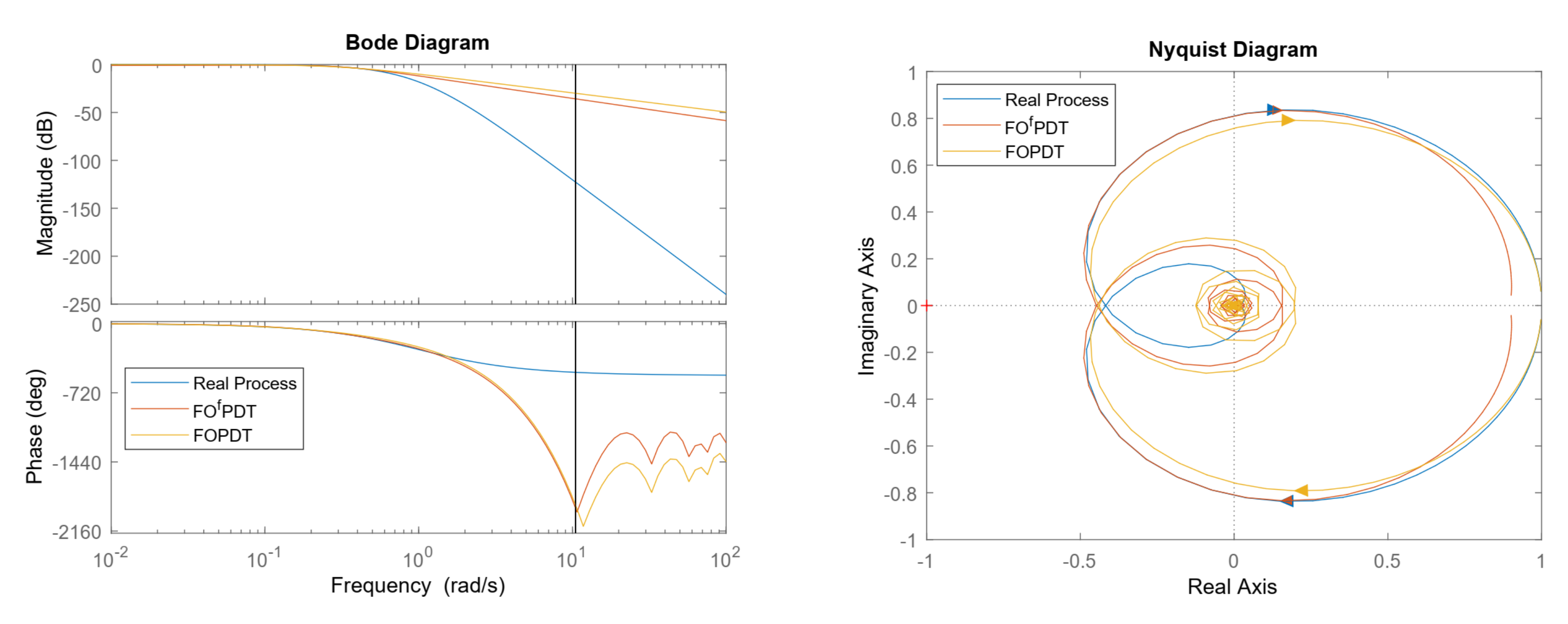
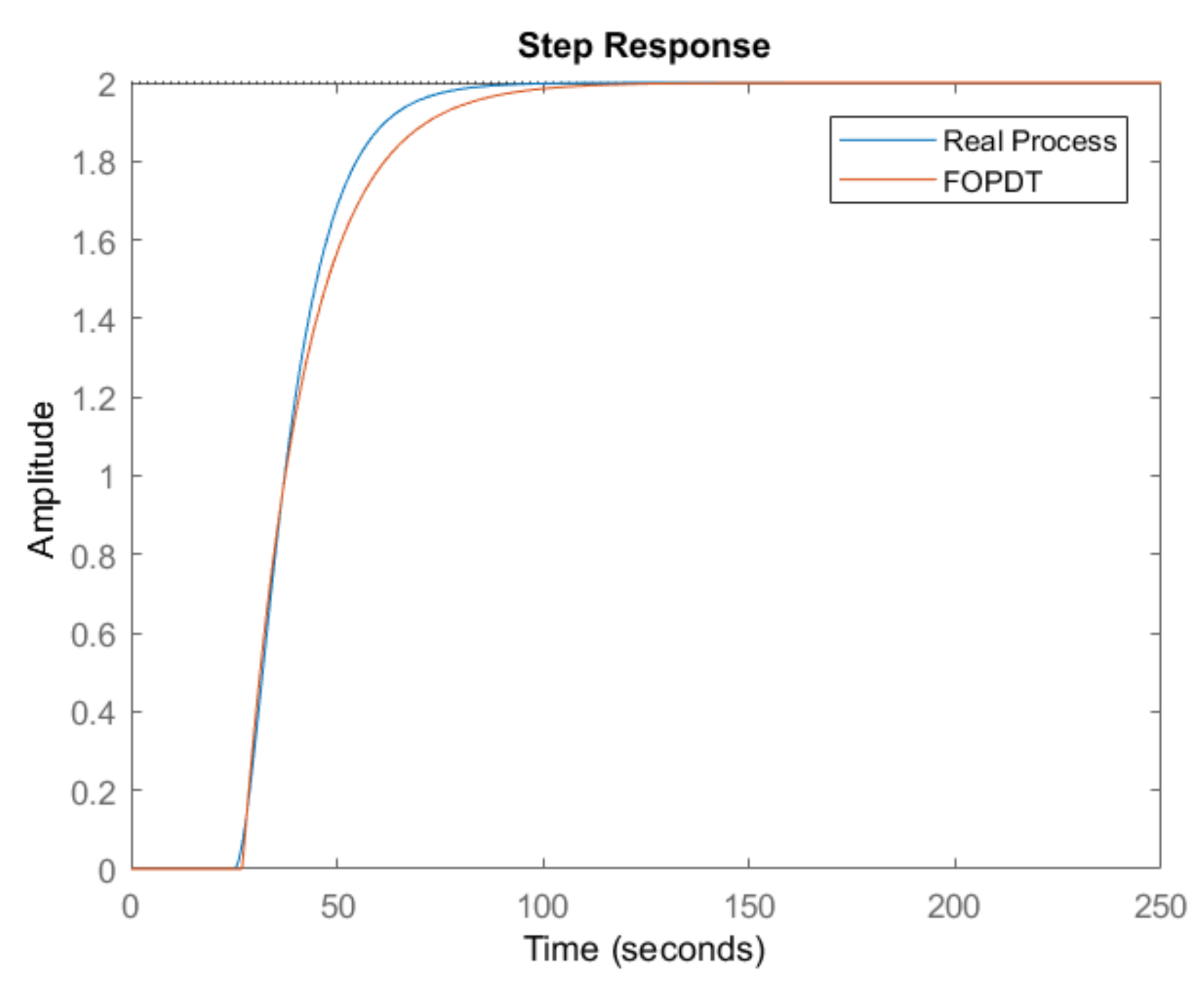
4.1.3. Delay Dominant Example

When approximations of FOPDT are used for dynamic step response from the real process, the processes are classified in three groups. This is based on the formula
τ = T T + T d
and the intervals defined as:
  • if τ ( 0 , 0.5 ) then the system is lag dominant;
  • if τ 0.5 then the system is balanced; and
  • if τ ( 0.5 , 1 ) then the system is delay dominant.
In [16] we discussed the process with significant time delay:
P ( s ) = 2 ( 5 s + 1 ) ( 10 s + 1 ) e 25 s
with sampling period T s = 0.3 and the FOPDT approximation given by
P a p ( s ) = 2 ( 15 s + 1 ) e 27 s
The step response is given in Figure 9. Notice that in practice, the FOPDT approximation is done by trial-and-error manner, and this particular approximation is very good.
The identified FO f PDT model has the form
P i d ( s ) = 1.8868 15.19 s 1.086 + 1 e 27.68 s
where no constraints have been put on the values of α . The stability margins are given in Table 3 below and the frequency response in terms of Bode and Nyquist plots in Figure 10, available with program in Supplementary Material. From the Nyquist diagram we conclude that the identified FO f PDT model outperforms by far the FOPDT approximated model.
Notable surveys of real life processes requiring fractional order transfer function models have been given in [30,31].

4.2. On Control Design

The initial properties of the system, such as PM and GM, will strongly influence the limitations of the closed loop bandwidth. The controller will have to bring in the loop response the difference between process features and a specified GM or/and PM by the user for the closed loop properties. Obviously, a system with a large PM will lessen the tight conditions on the controller design, enabling the possibility to achieve a better (larger) bandwidth with larger robustness than a process already closer to stability margins in terms of GM and PM. A complete analysis with theoretical insight has been given in [32,33] and for example, user defined PM based automatic tuning rules presented in [4,10,34].
In industrial control practice, the FOPDT model is used by process operators to detect basis features of the process such as time constant T, gain K and delay T d (artificially introduced by approximating high order dynamics or naturally present in process, or combination of both). Usually, industrial use does not identify this model form, but directly approximates it from data step response (see a comprehensive summary of industrial practice by ABB in [35]). If this model is introduced by the operator as information on the process to be controlled, a vast variety of automatic rules are directly available to design PID–forms of controllers. This has been exemplified in [11,21,22] and recently introduced with event-based control concepts for model identification in [36,37,38].
Alternatively, automatic tuning of controllers is based on harvesting information from experiment data such as a relay test, a sinusoidal test; see examples on real life processes in [7,27]. These newer methods use automatic optimization techniques, which move away from the hands-on training for process operators from earlier decades. With the availability of digital system control this is now possible to perform in efficient manner.
The FO f PDT form has been used to design control parameters in [16]. Such similar process transfer function models have been also used in many other recent works [6,15] to mention a few. A good textbook for design of fractional order controllers based on frequency response stability margin criterion is [4].
From a methodological point of view, the frequency response design is no different from loop shaping in optimal control design. The most commonly used form of controller is obviously the generalization of the classical PID controller structure to a fractional order in the form
P I D ( s ) = K p + K i s γ + K d s δ
with K p the proportional gain, K i the integral gain and K d the derivative gain and γ , δ their respective fractional orders. By their fractional order terms, this generalized PID controller form has two additional degrees-of-freedom when tuning is concerned. A geometrical interpretation of this form has been recently addressed in [39]. The control design can be applied as with any other model structure, based on frequency response characteristic. This poses not any difficulty as all four model structures presented in this paper have a frequency response which can be analytically calculated for the purpose of controller design.
In particular, the model generalizations are useful for control design purposes as the inequalities hold for conditions of critical frequency ω c when the phase of the system is −180°, i.e., the result of a relay feedback experiment. This is commonly employed in automatic tuning of PID-type controller parameter methods. Autotuning methods based on user defined specifications in frequency domain such as GM and PM have been given in [4,5] and recently in [8,28]. As in the numerical examples given in Table 2 and Table 3, the critical frequencies are very close to each other although the stability margins differ significantly among the sets of model structures. This implies that one model structure offers significantly improved stability margins to play with, while maintaining the same bandwidth. Consequently, it relaxes the conditions imposed on the set of solutions for controller design.
Recent surveys of real life processes requiring fractional order PID controllers have been given in [9,15,40,41,42]. The experimental works involving a closest form of the FO f PDT model for controller tuning purposes are very scarce, e.g., [25,43,44,45,46]. Closed loop control examples of FOPDT structures with fractional order time constant representative for real life processes has been given in [16].

4.3. On Deployment

When used in computer-based digital systems, the fractional order transfer functions of the model or of the controller, need to be discretized. An efficient method delivering a minimal integer order equivalent discretized model is given in [29] along with a Matlab (R2017a, MathWorks, Gent, Belgium, 2017) implemented software example. The advantage of the method is that discretization occurs directly from the transfer function in Laplace, making it very compact in terms of programming.
When analogue realizations are envisaged, this is also possible through special circuitry and elements with specific material properties, as provided in [43].
Fractional order controllers deployed in real time systems have been broadly used in experimental systems; see e.g., [21,22,42,47,48].
A notable review of numerical tools is given in [49].

5. Conclusions

In this paper we introduced a generalization of the classical first order plus dead time transfer function model and examined cases when the generalization has an advantage in terms of robustness when compared to its nominal form. The analytical study provided insight into the usefulness of the model as a function of frequency intervals of interest for the dynamic process at hand. A discussion section provides the reader with potential relevance for identification and control design purposes and points to relevant works where the model structures have been used in simulation and experimental studies. As the concept is newly emerging, opportunities arise to investigate the use of these models in practice for capturing real process dynamic characteristics and design controllers in frequency domain.

Supplementary Materials

The following are available online at https://www.mdpi.com/2227-9717/8/6/682/s1.

Author Contributions

Conceptualization, C.M.I.; methodology, C.I.M.; software, all authors; validation, all authors; formal analysis, all authors; writing—original draft preparation, C.M.I.; writing—review and editing, all authors; visualization, all authors; project administration, all authors. All authors have read and agreed to the published version of the manuscript.

Funding

The work of C. Ionescu has been supported by the Special Research Fund of Ghent University: MIMOPREC grant nr STG2018-020. The work of C. Muresan was supported by a grant of the Romanian National Authority for Scientific Research and Innovation, CNCS/CCCDI-UEFISCDI, project number PN-III-P1-1.1-TE-2016-1396, TE 65/2018.

Conflicts of Interest

The authors declare no conflict of interest.

Abbreviations

The following abbreviations are used in this manuscript:
FOPDTFirst Order Plus Dead Time
FO f PDTFirst Order Fractional Plus Dead Time
FOPDT f First Order Plus Dead Time Fractional
FO f PDT f First Order Fractional Plus Dead Time Fractional
SOPDTSecond Order Plus Dead Time
PIDProportional Integral Derivative (Control)
GMGain Margin
PMPhase Margin

Appendix A. Generic FOfPDT Model Identification

We give here a summary of the estimation method presented for the first time in [16] for the FOPDT and FO f PDT model structures. This particular methodology aims to fastforward the estimation optimization process by avoiding a full nonlinear in the parameter identification procedure, as the fractional order term α is apriori handled as explained above. The other advantage is that a sinusoidal test can be applied, which is easy to perform during the operation of the industrial process without disturbing its nominal operation in a disruptive way as a relay test may do. Further information of the sinusoidal test model identification for automatic tuning of controller parameters are given in [7].
The derivative of the classical FOPDT model is given by
d P ( s ) d s = K e T d s ( L s α + 1 ) 2 α L s α 1 + K e T d s ( L s α + 1 ) T d = K e T d s L s α + 1 α L s α 1 L s α + 1 + T d = P ( s ) α L s α 1 L s α + 1 + T d
Separating on the left hand the process and its slope gives:
d P ( s ) d s P ( s ) = α L s α 1 L s α + 1 + T d
The frequency domain representation of (A2) is given by
j d P ( j ω ) d ω P ( j ω ) = α L ( j ω ) α 1 L ( j ω ) α + 1 + T d = A + j B
with A and B the real and imaginary parts of the complex number j d P ( j ω ) d ω P ( j ω ) . Notice that the values of A and of B are known from the sine test.
A + j B = α L ( j ω ) α 1 L ( j ω ) α + 1 · L ( j ω ) α + 1 L ( j ω ) α + 1 + T d
which gives after multiplication
A + j B = α j ω [ ( j ) α ω α L + ω 2 α L 2 ] 1 + [ ( j ) α + ( j ) α ] ω α L + ω 2 α L 2 + T d
Supposing α is apriori given (e.g., in a loop for determined interval values), the complex number j α in (A5) can be expressed as
j α = e j π 2 α = cos ( π 2 α ) + j sin ( π 2 α )
and denoting X = ω α L we can separate the real and imaginary parts in (A5) as:
A = α ω sin ( π 2 α ) X 1 + 2 cos ( π 2 α ) X + X 2 + T d
and
B = α ω cos ( π 2 α ) X + X 2 1 + 2 cos ( π 2 α ) X + X 2
Expression (A8) can be written as:
B + α ω X 2 + 2 B + α ω cos ( π 2 α ) X + B = 0
from which X is obtained ( α is given, B is known, and ω = ω ¯ ), hence
L = X ω α
From the expression of the real part (A7), knowing X, we can obtain the time delay T d . Plugging the calculated values for L and D and the known α value into FOPDT model (with s = j ω ¯ ), it gives K. At this moment, all parameters of (1) are known. Adding a fitting cost to this procedure for the various values of α , the minimal cost delivers the final model parameter values.
The algorithm is executed for a pre-defined interval in small steps (e.g., Δ α = 0.001 ), i.e., any interval set by the GM and PM inequalities. The final solution is given by that α value for which the following conditions are fulfilled:
( K , L ) R ,   and   ( L , T d ) > 0
Notice that if L R , then it follows from (A7) that also T d R . For all examples tested hitherto, of which three selected representative ones are given in this paper, an unique solution for α was found which satisfied (A11).
The result is thus an FO f PDT model, which has at the test frequency ω ¯ the same frequency response value and the same frequency response slope as the real process.

References

  1. Alfaro, V.M. PID controllers’ fragility. ISA Trans. 2007, 46, 555–559. [Google Scholar] [CrossRef] [PubMed]
  2. Samad, T. A survey on industry impact and challenges thereof. IEEE Control Syst. Mag. 2017, 37, 17–18. [Google Scholar]
  3. Ionescu, C.; Copot, D. Hands-on MPC tuning for industrial applications. Bull. Pol. Acad. Sci. Tech. Sci. 2019, 67, 925–945. [Google Scholar] [CrossRef]
  4. Monje, C.; Chen, Y.; Vinagre, B.; Xue, D.; Feliu, V. Fractional Order Systems and Controls; Springer: London, UK, 2010. [Google Scholar]
  5. Padula, F.; Visioli, A. Advances in Robust Fractional Control; Springer: Cham, Switzerland, 2015. [Google Scholar]
  6. Petras, I. Fractional Order Nonlinear Systems; Springer: Berlin, Germany, 2011. [Google Scholar]
  7. De Keyser, R.; Muresan, C.; Ionescu, C. Universal direct tuner for loop control in industry. IEEE Access 2019, 7, 81308–81320. [Google Scholar] [CrossRef]
  8. Copot, C.; Muresan, C.; Ionescu, C. Image-Based and Fractional-Order Control for Mechatronic Systems. Series: Advances in Industrial Control; Springer: Berlin, Germany, 2020. [Google Scholar]
  9. Dastjerdi, A.; Vinagre, B.; Chen, Y.Q.; HosseinNia, S. Linear fractional order controllers; a survey in the frequency domain. Annu. Rev. Control 2019, 47, 51–70. [Google Scholar] [CrossRef]
  10. Kristiansson, B.; Lennartson, B. Robust and optimal tuning of PI and PID controllers. IEE Proc. Control Theory Appl. 2002, 149, 17–25. [Google Scholar] [CrossRef]
  11. Åström, K.; Hägglund, T. Advanced PID Control; Instrumentation, Systems and Automation Society (ISA): Atlanta, GA, USA, 2006. [Google Scholar]
  12. Padula, F.; Visioli, A. On the fragility of fractional-order PID controllers for FOPDT processes. ISA Trans. 2016, 60, 228–243. [Google Scholar] [CrossRef] [PubMed]
  13. Li, X.; Chen, Y.; Podlubny, I. Mittag-Leffler stability of fractional order nonlinear dynamic systems. Automatica 2009, 45, 1965–1969. [Google Scholar] [CrossRef]
  14. Luo, Y.; Chen, Y. Fractional order [proportional derivative] controller for a class of fractional order systems. Automatica 2009, 45, 2446–2450. [Google Scholar] [CrossRef]
  15. Birs, I.; Muresan, C.I.; Nascu, I.; Ionescu, C.M. A survey of recent advances in fractional order control for time delay systems. IEEE Access 2019, 7, 30951–30965. [Google Scholar] [CrossRef]
  16. De Keyser, R.; Ionescu, C. Minimal information based, simple identification method of fractional order systems for model based control applications. In Proceedings of the Asian Conference on Control, Gold Coast, Australia, 17–20 December 2017; pp. 1411–1416. [Google Scholar]
  17. Juchem, J.; Dekemele, K.; Chevalier, A.; Loccufier, M.; Ionescu, C. First order plus frequency dependent delay modelling: New perspective or mathematical curiosity? In Proceedings of the Conference on System Man and Cybernetics, Bari, Italy, 6–9 October 2019; pp. 2025–2030. [Google Scholar]
  18. Oustaloup, A. Diversity and Non-Integer Differentiation for System Dynamics (Control Systems and Industrial Engineering); Wiley: London, UK, 2014. [Google Scholar]
  19. Baleanu, D.; Tenreiro Machado, J. (Eds.) Fractional Dynamics and Control; Springer: New York, NY, USA, 2012. [Google Scholar]
  20. Nise, N. Control System Engineering, 6th ed.; John Wiley & Sons: Hoboken, NJ, USA, 2011. [Google Scholar]
  21. Copot, D.; Ghita, M.; Ionescu, C. Simple alternatives to PID–type control for processes with variable time delay. Processes 2019, 7, 146. [Google Scholar] [CrossRef] [Green Version]
  22. Copot, D.; Ionescu, C. A fractional order controller for delay dominant systems: Application to a continuous casting line. J. Appl. Nonlinear Dyn. 2019, 8, 67–78. [Google Scholar] [CrossRef]
  23. Birs, I.; Copot, D.; Pilato, C.; Ghita, M.; Caponetto, R.; Muresan, C.; Ionescu, C. Experiment design and estimation methodology of varying properties for non-Newtonian fluids. In Proceedings of the Conference on System Man and Cybernetics, Bari, Italy, 6–9 October 2019; pp. 324–329. [Google Scholar]
  24. Birs, I.; Copot, D.; Ghita, M.; Muresan, C.; Ionescu, C. Fractional-order modelling of impedance measurements in a blood resembling experimental setup. In Proceedings of the Conference on System Man and Cybernetics, Bari, Italy, 6–9 October 2019; pp. 898–903. [Google Scholar]
  25. Birs, I.; Muresan, C.; Copot, D.; Nascu, I.; Ionescu, C. Identification for control of suspended objects in non-Newtonian fluids. Fract. Calc. Appl. Anal. 2019, 22, 1378–1394. [Google Scholar] [CrossRef]
  26. De Keyser, R.; Muresan, C. Robust estimation of a SOPDT model from highly corrupted step response data. In Proceedings of the European Control Conference, Naples, Italy, 25–28 June 2019; pp. 818–823. [Google Scholar]
  27. Berner, J.; Soltesz, K.; Hägglund, T.; Åström, K. Autotuner Identification of TITO Systems Using a Single Relay Feedback Experiment; IFAC Papers On-Line; IFAC, Ed.; IFAC World Congress: Prague, Czech Republic, 2017; pp. 5332–5337. [Google Scholar] [CrossRef]
  28. De Keyser, R.; Muresan, C.; Ionescu, C. A novel auto–tuning method for fractional order PI/PD controllers. ISA Trans. 2016, 92, 268–275. [Google Scholar] [CrossRef] [PubMed]
  29. De Keyser, R.; Muresan, C.; Ionescu, C. An efficient algorithm for low-order direct discrete-time implementation of fractional order transfer functions. ISA Trans. 2018, 74, 229–238. [Google Scholar] [CrossRef] [PubMed]
  30. Ionescu, C.; Lopes, A.; Copot, D.; Tenreiro Machado, J.; Bates, J. The role of fractional calculus in modeling biological phenomena: A review. Commun. Nonlinear Sci. Numer. Simul. 2017, 51, 141–159. [Google Scholar] [CrossRef]
  31. Sun, H.; Zhang, Y.; Baleanu, D.; Chen, W. A new collection of real world applications of fractional calculus in science and engineering. Commun. Nonlinear Sci. Numer. Simul. 2018, 64, 213–231. [Google Scholar] [CrossRef]
  32. Ionescu, C.; De Keyser, R. The next generation of relay-based PID autotuners (part 1): Some insights on the performance of simple relay-based PID autotuners. In Proceedings of the IFAC Advances in PID Control, Brescia, Italy, 28–30 March 2012; pp. 122–127. [Google Scholar] [CrossRef] [Green Version]
  33. De Keyser, R.; Joita, O.; Ionescu, C. The next generation of relay-based PID autotuners (part 2): A simple relay-based PID autotuner with specified modulus margin. In Proceedings of the IFAC Advances in PID Control, Brescia, Italy, 28–30 March 2012; pp. 128–133. [Google Scholar] [CrossRef] [Green Version]
  34. De Keyser, R.; Dutta, A.; Hernandez, A.; Ionescu, C. A specifications based PID autotuner. In Proceedings of the Conference on Control Applications, Dubrovnik, Croatia, 3–5 October 2012; pp. 1621–1626. [Google Scholar] [CrossRef]
  35. Starr, K. Single Loop Control Methods; ABB Process Automation Service: Baden, Switzerland, 2016. [Google Scholar]
  36. Sánchez, J.; Guinanldo, M.; Visioli, A.; Dormido, S. Identification of process transfer function parameters in event-based PI control loops. ISA Trans. 2018, 75, 157–171. [Google Scholar] [CrossRef] [PubMed]
  37. Sánchez, J.; Guinanldo, M.; Visioli, A.; Dormido, S. Enhanced event-based identification procedure for process control. Ind. Eng. Chem. Res. 2018, 57, 7218–7231. [Google Scholar] [CrossRef]
  38. Merigo, L.; Beschi, M.; Padula, F.; Visioli, A. A noise filtering event generator for PIDPlus controllers. J. Frankl. Inst. 2018, 355, 774–802. [Google Scholar] [CrossRef]
  39. Tejado, I.; Vinagre, B.; Traver, J.; Prieto–Arranz, J.; Nuevo–Gallardo, C. Back to basics: Meaning of the parameters of fractional order PID controllers. Mathematics 2019, 7, 530. [Google Scholar] [CrossRef] [Green Version]
  40. Cajo Diaz, R.; Mac Thi, T.; Plaza Guingla, D.; Copot, C.; De Keyser, R.; Ionescu, C. A survey on fractional order control techniques for unmanned aerial and ground vehicles. IEEE Access 2019, 7, 66864–66878. [Google Scholar] [CrossRef]
  41. Dastjerdi, A.; Saikumar, N.; HosseinNia, S. Tuning guidelines for fractional order PID controllers: Rules of thumb. Mechatronics 2018, 56, 26–36. [Google Scholar] [CrossRef]
  42. Chevalier, A.; Francis, C.; Copot, C.; Ionescu, C.; De Keyser, R. Fractional order PID design: Towards transition from state-of-art to state-of-use. ISA Trans. 2019, 84, 178–186. [Google Scholar] [CrossRef] [PubMed]
  43. Biswas, K.; Bohannan, G.; Caponetto, R.; Lopes, A.M.; Tenreiro Machado, J. Fractional-Order Devices; Springer Nature: Cham, Switzerland, 2017. [Google Scholar]
  44. Barbosa, R.; Tenreiro Machado, J.; Ferreira, I. Tuning of PID controllers based on Bode’s ideal transfer function. Nonlinear Dyn. 2004, 38, 305–321. [Google Scholar] [CrossRef]
  45. Jesus, I.; Tenreiro Machado, J. Fractional control of heat diffusion systems. Nonlinear Dyn. 2008, 54, 263–282. [Google Scholar] [CrossRef] [Green Version]
  46. HosseinNia, S.; Tejado, I.; Vinagre, B. Fractional-order reset control: Application to a servomotor. Mechatronics 2013, 23, 781–788. [Google Scholar] [CrossRef]
  47. Muresan, C.; Folea, S.; Birs, I.; Ionescu, C. A novel fractional order model and controller for vibration supression in flexible smart beam. Nonlinear Dyn. 2018, 93, 525–541. [Google Scholar] [CrossRef]
  48. Zhao, S.; Cajo Diaz, R.; De Keyser, R.; Ionescu, C. The potential of fractional order distributed MPC applied to steam/water loop in large scale ships. Processes 2020, 8, 451. [Google Scholar] [CrossRef] [Green Version]
  49. Li, Z.; Liu, L.; Dehghan, S.; Chen, Y.Q.; Xue, D. A review and evaluation of numerical tools for fractional calculus and fractional order controls. Int. J. Control. Spec. Issue Appl. Fract. Calc. Model. Anal. Des. Control Syst. 2017, 90, 1165–1181. [Google Scholar] [CrossRef] [Green Version]
Figure 1. Surface of solutions for Equation (14) for G M 2 > G M 1 .
Processes 08 00682 g001
Figure 2. Surface of solutions for denominator of Equation (17).
Processes 08 00682 g002
Figure 3. Surface of solutions for Equation (17) for P M 2 > P M 1 .
Processes 08 00682 g003
Figure 4. Surface of solutions for Equation (24) for P M 3 > P M 1 .
Processes 08 00682 g004
Figure 5. Nyquist plot of the frequency response of the four model structures, starting from FOPDT (top) to FO f PDT f (bottom). All model structures have K = 1 , T = 1 and T d = 1 .
Processes 08 00682 g005
Figure 6. Scheme of the experimental procedure to obtain the (sine) signals y ( t ) and y ¯ ( t ) and compute the phase slope of the process at the phase crossover frequency (or other frequency), from [28].
Processes 08 00682 g006
Figure 7. Step response for the real high order system and the FOPDT approximation model.
Processes 08 00682 g007
Figure 8. Frequency response of the real process and the FOPDT and FO f PDT model estimations.
Processes 08 00682 g008
Figure 9. Step response for the real high order system and the FOPDT approximation model.
Processes 08 00682 g009
Figure 10. Frequency response of the real process and the FOPDT and FO f PDT model estimations.
Processes 08 00682 g010
Table 1. Non-exhaustive summary of published reports where the various forms of FOPDT generalization has been employed on a real life process with experimental data. NMP: non-minimum phase; MIMO: multiple input multiple output.
ProcessModelReference
high order, delay dominantFOPDT[4,21,22]
NMP, open loop unstable, MIMO, poorly dampedFOPDT[3]
high orderFO f PDT[23,24,25]
high orderFOPDT f [17]
Table 2. Stability margins for the three process transfer functions.
ProcessGMPM ω p ω g
Real Process2.3741-0.5770-
FO f PDT2.2348-0.6018-
FOPDT2.2612-0.6758-
Table 3. Stability margins for the three process transfer functions.
ProcessGMPM ω p ω g
Real Process0.7011−97.38310.08240.1330
FO f PDT0.7011−101.78940.08240.1360
FOPDT0.7996−58.69130.08310.1154

