An Adjective Selection Personality Assessment Method Using Gradient Boosting Machine Learning

Abstract

Goldberg’s 100 Unipolar Markers remains one of the most popular ways to measure personality traits, in particular, the Big Five. An important reduction was later preformed by Saucier, using a sub-set of 40 markers. Both assessments are performed by presenting a set of markers, or adjectives, to the subject, requesting him to quantify each marker using a 9-point rating scale. Consequently, the goal of this study is to conduct experiments and propose a shorter alternative where the subject is only required to identify which adjectives describe him the most. Hence, a web platform was developed for data collection, requesting subjects to rate each adjective and select those describing him the most. Based on a Gradient Boosting approach, two distinct Machine Learning architectures were conceived, tuned and evaluated. The first makes use of regressors to provide an exact score of the Big Five while the second uses classifiers to provide a binned output. As input, both receive the one-hot encoded selection of adjectives. Both architectures performed well. The first is able to quantify the Big Five with an approximate error of 5 units of measure, while the second shows a micro-averaged f1-score of 83%. Since all adjectives are used to compute all traits, models are able to harness inter-trait relationships, being possible to further reduce the set of adjectives by removing those that have smaller importance.

1. Introduction

People react differently when experiencing the same situations. This behavioural diversity may be due to one’s experience, knowledge or even personality. Indeed, several studies have already established a relationship between a person’s personality and aggressive reactions [1], work performance [2] or infidelity [3], just to name a few. Semantically, personality may be defined as a set of characteristics that refer to individual differences in ways of thinking, feeling and behaving [4]. Personality has a great impact in the the way we live our lives, either by the way we behave, feel or interact with others. Hence, there has always been great interest in model, or quantify, a person’s personality using either qualitative or quantitative metrics. Nowadays, there are several accepted tests that allow a psychological assessment of a person. Such tests may be performed in the scope of psychology appointments, job interviews or psychometric evaluations. These tests are mainly conducted by trained professionals that are able to properly interpret their results.

1.1. Personality Assessment

Personality assessment is a well defined process that can help unveil how a person may react to different, unexpected, situations [5]. Several personality tests are available such as HEXACO-60 [6], Myers-Briggs Type Indicator [7], the Enneagram of Personality [8] and NEO-personality-inventory (NEO-PI-R) [9]. Goldberg’s 100 Unipolar Markers’ Test [10] is yet another test that consists of a total of 100 adjectives, or markers, that the subject must rate on how they relate to each adjective, with 1 being Extremely Inaccurate and 9 Extremely Accurate. Among the full set of markers one may find adjectives such as talkative, sympathetic, careless, envious or deep. Goldberg’s test allows one to measure five domains, in particular, Surgency, Agreeableness, Conscientiousness, Emotional Stability and Intellect. Different domains have also been proposed. The OCEAN model, on the other hand, consists of the following five factors [11,12]:

• Openness: related to one’s curiosity, imagination and openness to new experiences. Higher values usually emerge on people that enjoy new adventures and ideas. On the other hand, lower values tend to emerge on more conservative people;
• Conscientiousness: related to self-discipline, being careful and diligent, organised and consistent, pursuing long-term goals. Less conscientious people tend to be more spontaneous and imaginative;
• Extraversion: related to a state where a person seeks stimulation from being with others instead of being alone. Extroverted people tend to be energetic and talkative, while introverted ones are reserved and prefer not to be the centre of attention;
• Agreeableness: related to behavioural characteristics such as being kind and sympathetic. Agreeable people tend to be friendly, cooperative and empathetic. Non-agreeable people are less cooperative, and more competitive and suspicious;
• Neuroticism (opposite of Stability): related to being moody and showing signs of emotional instability. Neurotic people tend to be stressed and nervous. Non-neurotic people tend to be calmer and more emotionally stable [12].

Goldberg’s test consist of 100 unipolar markers that must be quantified by a subject. An important reduction to the set of markers was performed by Gerard Saucier with The Mini-Marker test, using a sub-set of 40 markers to assess the Big Five with an acceptable performance, leading to the use of less difficult markers and lower inter-scale correlations [13]. Saucier’s test uses the same rating scale, being made of five disjoint-sets of eight unipolar markers each:

• Intellect or Openness trait is made of six positively weighted adjectives (intellectual, creative, complex, imaginative, philosophical and deep) and two negative ones (average and ordinary);
• Conscientiousness trait is made of four positively weighted adjectives (systematic, practical, efficient and orderly) and four negative ones (disorganised, careless, inefficient and sloppy);
• Extraversion trait is made of four positively weighted adjectives (extraverted, talkative, energetic and bold) and four negative ones (shy, quiet, withdrawn and bashful);
• Agreeableness trait is made of four positively weighted adjectives (kind, cooperative, sympathetic and warm) and four negative ones (cold, harsh, rude and distant);
• Emotional Stability trait is made of two positively weighted adjectives (relaxed and mellow) and six negative ones (moody, temperamental, envious, fretful, jealous and touchy).

1.2. Machine Learning for Personality Assessment

During these last years, Machine Learning (ML) has been raising to prominence. In fact, the use of ML models to predict personality traits has gain significant popularity within the field of Affective Computing, with several studies having already engaged on conceiving ML models for personality assessment [12,14,15,16]. In 2017, Majumder et al. conceived and evaluated Deep Learning (DL) models to assess personality from text. They conceived and fit a total of five artificial neural networks (ANN), one for each of the Big Five personality traits. All networks had the same architecture, with each ANN behaving as a binary classifier to predict whether the trait was positive or negative [14]. As dataset the authors used James Pennebaker and Laura King’s stream-of-consciousness essay dataset, which contains 2468 anonymous essays tagged with the binary value for each of the Big Five [17]. This dataset seems, however, to be currently unavailable. In fact, several datasets containing anonymized psychological assessments seem to have been locked, or closed, such as the one provided by the myPersonality platform (myPersonality.org), a platform that made available a dataset containing textual social media data and from where several studies emerged, being essentially focused on modelling personality traits based on language-based information [18,19].

In a slightly different domain, in 2017, Yu and Markov conceived and evaluated several DL models to learn suitable data representation for personality assessment, using facebook status update data. This dataset consisted of raw text, user’s information and standard Big Five labels, which were obtained using self-assessment questionnaires [15]. In fact, it is possible to find several studies focused on inferring personality based on social media feeds. For instance, Kosinski et al. (2014) focused on examining how an individual’s personality manifests in his/her online behaviour, in particular, the website he/she visits and his/her Facebook activity. The expectation is that web activity combined with social media data may bring unbiased insights, since social media feeds may carry an intention of self-enhancement and positivity [12]. The used dataset was obtained from myPersonality. The obtained results showed psychologically meaningful links between individuals’ personalities, website preferences and social media data. The potential applications of these works are essentially related with targeted advertising and personalised recommender systems, which take into consideration one’s personality to deliver useful content.

In 2012, Sumner et al., based on Twitter use, focused on identifying signals of the Dark Triad, i.e., the anti-social traits of Narcissism, Machiavellianism and Psychopathy. Almost three thousand Twitter users, from 89 countries, participated in the study, with an in-built Twitter application being developed to collect self-reported ratings on the Short Dark Triad questionnaire, which measures the anti-social traits, and the Ten Item Personality Inventory (TIPI) test, which measures the Big Five. The authors conclude that even though possible to examine large groups of people, the conceived ML models behave poorly when applied to individuals, being imprecise when predicting Dark Triad traits just from Twitter activity [16].

Another study, performed by Cerasa et al. (2018), focused on conceiving and evaluating ML models to identify individuals with gambling disorder. To build the dataset, a set of healthy and sick individuals were asked to perform the NEO-PI-R test, an operationalization of the five factor model. The authors employed Classification and Regression Trees (CART) achieving interesting performances evaluated using the area under the curve (AUC). In fact, the best candidate model was able to identify individuals with gambling disorder with an AUC of approximately 77% [20].

On the other hand, studies have been performed where audio and video data are used by DL-based models to predict personality [21]. One study, performed by Levitan et al. (2016), focused on the automatic identification of traits such as gender, deception and personality using acoustic-prosodic and lexical features [22]. In particular, the authors focused on automatic detection of deception. The authors used Columbia deception corpus, which consists of deceptive and non-deceptive speech from standard American-English and Mandarin-Chinese native speakers, including more than one hundred hours of speech with self-identified truth/lie labels [23]. The authors then collected demographic data from each subject and administered a NEO-FFI personality test to access the Big Five. Each trait was binned as a three-class classification problem (low, medium and high), which created an highly unbalanced dataset since the majority of subjects fell into the medium class. Hence, to compare models’ performances the authors used f-scores to obtain a meaningful comparison. Several ML models and feature sets were experimented, with AdaBoost and Random Forests being the best performing classifiers for personality assessment [22].

Another study, performed by Gurpinar et al. (2016), focused in using DL to predict the Big Five of faces appearing in videos [24]. The authors employed transfer-learning and Convolutional Neural Networks to extract facial expressions, as well as ambient information. The conceived models were evaluated on the ChaLearn Challenge Dataset on First Impression Recognition, which consists of ten thousand clips collected from more that five thousand YouTube videos. The label of each clip corresponds to the Big Five personality traits of the person appearing in that clip. Their best candidate model achieved an accuracy of over 90% on the test set [24].

It is also usual to find the use of different data sources combined through means of data fusion for personality assessment. Indeed, personality assessment from multi-modal data has been assuming a greater importance in the computer vision field [25]. For instance, Gucluturk et al. (2017), aimed to analyse what features are used by personality trait assessment models when making predictions, conducting several experiments that characterised audio and visual information that drive such predictions [25]. On the other hand, Zhang et al. (2016) proposed a Deep Bimodal Regression framework to capture rich information from both the visual and audio aspects of videos, winning the ChaLearn Looking at People challenge. Convolutional Neural Networks were conceived to exploit visual cues, while linear regressors where used for audio [26].

1.3. Hypothesis and Paper Structure

Many studies have already engaged on using ML or DL for personality assessment using images, videos, audio or text. However, to the best of our knowledge, we are the first to apply ML to reduce the complexity of a test. In fact, the working hypothesis is that it is possible to use ML-based modes to further reduce Saucier’s Mini-Marker to a "game of words" where the subject, instead of rating forty adjectives, only has to select those he relates the most, removing the need to rate adjectives. The proposed Adjective Selection to Assess Personality (ASAP) method replaces the entire process of rating adjectives by an adjective selection process. The goal is to reduce the complexity of tests, the time it takes to perform a test, and to make the test more attractive and easier to implement in current and future technological platforms. Hence, this study aims to conceive, tune and evaluate two distinct Gradient Boosting ML architectures to quantify an individual’s personality based on his/her choice of adjectives. Due to the non-availability of data, a web platform was developed and place online, being responsible for the entire data collection process. To conduct experiments on non-data scarce environments, data augmentation techniques were designed and implemented to produce a second dataset, which was also evaluated.

The remainder of this paper is structured as follows, viz. Section 2 describes the material and methods, in particular the developed platform for data collection, data exploration, the implemented data augmentation techniques as well as the conceived ML architectures, the experimental setup and the conducted experiments. Section 3 summarises the obtained results, providing a concise description of the experimental results and their interpretation. Section 4 presents and discusses the results and their interpretation in the perspective of previous studies and of the working hypothesis, depicting the main conclusions and pointing future research directions.

2. Materials and Methods

Due to the non-availability of data and the particularities of the proposed ASAP method, we were required to develop a web platform for data collection, requesting subjects to rate adjectives and select those describing them the most. This allowed us to build a dataset containing self-reported ratings on Saucier’s Mini-Marker test, the corresponding values of the Big Five as well as the adjectives selected by the subjects. The next lines describe in detail the developed platform, exploring and explaining the collected dataset and the implemented data augmentation techniques. It also details the conceived ML architectures and the experimental setup.

2.1. Dataset

The dataset used in this study is available, in its raw state, in an online repository (https://github.com/brunofmf/Datasets4SocialGood), under a MIT license.

2.1.1. Data Collection

To bring this study to a fruitful conclusion, we were required to collect a dataset from where we could derive conclusions. Hence, a platform was conceived and made available online (http://crowdsensing.di.uminho.pt/). The platform displays all 40 adjectives used by Saucier’s Mini-Marker test, asking the subject to rate each one. It also allows the subject to select a set of adjectives that describe him the most. Figure 1 depicts the main page of the conceived platform. The subject can then get the test results and obtain the value of each personality trait.

The platform provides a rationale to explain the subject how he/she is contributing to the study. No personal data are stored neither it is possible to link subjects to their answers - only information about age, genre and language are stored, and only if the user explicitly provides it. The platform is available online and any person can access and use it. It was published online on 21 September 2018. The platform was shared among a diversified population, using social media and university’s mailing lists. Data was also collected in person, which allowed us to increment the dataset size with records containing both the ratings and the selected list of adjectives.

To facilitate the data collection process, the developed platform allows subjects to perform Saucier’s Mini-Markers in three distinct languages. All translations were performed by three Portuguese and Spanish native speakers fluent in English, all university professors. It should also be highlighted that this study does not aim to examine the psychometric properties of the Portuguese or Spanish versions neither to provide sound validity evidence for the performed translations (even though Tau-Equivalent estimates of score reliability are later examined). The assumption is that ML models are able to quantify or qualify the traits without requiring any contextual information about region, genre, language or age of the subjects.

2.1.2. Data Exploration

The collected dataset contains 255 observations. Each observation is made of 50 features, viz, age, genre, language, 40 adjectives, 5 personality traits, the selected adjectives and the creation date. The features age, adjectives and personality traits are integers. The genre is a binary attribute and language is either es, en or pt. On the other hand, the selected adjectives feature consists of a string where the selected adjectives are comma separated.

Table 1. Features available in the collected dataset.

#	Feature	#	Feature	#	Feature
1	age	18	philosophical	35	cold
2	genre	19	bashful	36	disorganized
3	language	20	warm	37	temperamental
4	talkative	21	inefficient	38	complex
5	sympathetic	22	touchy	39	extraverted
6	orderly	23	creative	40	rude
7	envious	24	energetic	41	efficient
8	deep	25	cooperative	42	fretful
9	withdrawn	26	practical	43	imaginative
10	harsh	27	jealous	44	extraversion_trait
11	careless	28	intellectual	45	agreeableness_trait
12	relaxed	29	quiet	46	conscientiousness_trait
13	average	30	distant	47	stability_trait
14	bold	31	sloppy	48	openess_trait
15	kind	32	mellow	49	selected_attr
16	systematic	33	ordinary	50	creation_date
17	moody	34	shy

presents all available features in the collected dataset.

In the final dataset, 159 observations have the selected_attr feature filled with the selected adjectives. On the other hand, 96 observations only have the adjectives’ ratings. A few observations have adjectives rated with the value 0. 200 observations belong to male subjects, while 55 belong to female ones. Only two languages were used: 220 observations were done in Portuguese while 35 were done in English. More than 90% of the observations were collected in 2019. The mean age value is of 30.1 years.

Adjectives with lower mean value are essentially related to negative ones such as rude, with 3.13, inefficient, with 3.26, and ordinary, with 3.28. The adjectives that have higher mean value are kind, with 6.004, imaginative, with 6, and cooperative, with 5.73. Mean standard deviation of the 40 adjectives is 2.5, with the lower value being 0 and the maximum 9. Mean skewness is of 0.03, representing a symmetrical distribution. Mean kurtosis is of −0.98, representing a somewhat “light-tailed” dataset in regard to the 40 adjectives. In regard to the Big Five (

Table 2. Descriptive statistics for the Big Five.

	Openness	Conscientiousness	Extraversion	Agreeableness	Stability
Nº of Items	8	8	8	8	8
Mean	44.976	46.476	39.428	47.148	46.140
Median	46	47	40	48	46
Standard Deviation	10.315	10.547	10.017	10.056	8.860
Skewness	−0.212	−0.207	−0.135	−0.216	−0.047
Kurtosis	−0.260	−0.492	−0.344	−0.328	−0.484
Coefficient alpha	0.62	0.61	0.56	0.58	0.42

), the one having lower mean value is Extraversion, with Agreeableness being the one with higher mean value. Mean standard deviation of all traits is of approximately 10 units of measure. The coefficient alpha for the forty items is of 0.82 [27]. For each individual trait, the Tau-Equivalent estimates of score reliability are lower, specially for the Stability factor. Except for the selected_attr feature, no missing values are present in the dataset.

With all features assuming a non-Gaussian distribution (under the Kolmogorov-Smirnov test with $p<0.05$), the non-parametric Spearman’s rank correlation coefficient was used. A few pairs of correlated features, in the form (trait, adjective), appear in the dataset. This is in line with expectations since the Big Five are mathematically based on the adjectives. Higher correlations appear for the pairs (Agreeableness, Warm), (Conscientiousness, Efficient), (Openess, Complex) and (Extraversion, Extraverted).

The selected_attr feature consists of a string where adjectives are separated by commas. An example of a valid value would be "Talkative, Sympathetic, Kind, Energetic, Jealous, Intellectual, Extraverted, Efficient, Fretful". From all 159 observations that have the selected_attr feature filled, 157 are unique values meaning that only three subjects chose the same adjectives. Interestingly, all adjectives were selected at least once. In fact, the least selected adjectives were ordinary, which was selected 14 times, touchy, 18 times, rude, 19 times, cold and fretful, 23 times. These are, essentially, adjectives with negative connotation. On the opposite spectrum, kind was selected 67 times, imaginative, 59 times, sympathetic, 58 times, creative, 57 times, and withdrawn, 56 times (Figure 2). Excluding those who opt not to select adjectives, 10 subjects only chose one adjective to describe themselves, while 14 subjects selected fifteen, or more, adjectives. The mean value is of approximately ten selected adjectives per subject.

Approximately 38% of the total number of observations do not have adjectives selected. To overcome this issue, it becomes important to understand the relation between selecting an adjective and its respective rating. For instance, considering all subjects that selected the adjective efficient, the mean rating of that same adjective is of 5.794. On the other hand, the mean rating of the sloopy adjective considering all subjects that selected that adjective is of 8. This tells us that sloopy tends to be selected when receiving higher ratings. On the other hand, efficient is selected even with average ratings. The overall mean, 7.448, tells us that, as expected, adjectives tend to be selected when receiving high values. Figure 3 depicts the mean rating values to set an adjective as selected.

To discover relations between the selected adjectives, a ML and a pattern mining method, entitled as Association Rules Learning (ARL), was applied. ARL does not consider the order of the items, neither extract individual’s preference, but, instead, looks for frequent itemsets. The goal is to find associations and correlations between adjectives that were selected to describe subjects. In particular, the APRIORI algorithm was used to analyse the list of selected adjectives, and provide rules in the form Antecedent -> Consequent, where -> may be read as "implies". To find these rules, three distinct metrics were used: Support, which gives an idea of how frequent an itemset is in all existing transactions, helping identifying rules worth considering; Confidence, an indication of how often a rule has been found to be true; and Lift, which measures how much better the rule is at predicting the presence of an adjective compared to just relying on the raw probability of the adjective in the dataset. The returned rules go both ways, i.e., if A implies B then the reverse is also true.

Table 3. Rules with support higher than 0.15 using Association Rules Learning and the APRIORI algorithm.

Support	Confidence	Lift	Antecedent		Consequent
0.195	0.525	1.466	Creative	–>	Imaginative
0.189	0.508	1.207	Kind	–>	Imaginative
0.176	0.418	1.146	Sympathetic	–>	Kind
0.170	0.551	1.511	Sympathetic	–>	Relaxed
0.170	0.491	1.394	Withdrawn	–>	Intellectual
0.170	0.491	1.165	Kind	–>	Intellectual
0.170	0.540	1.281	Kind	–>	Shy
0.164	0.464	1.273	Sympathetic	–>	Withdrawn
0.164	0.634	1.505	Kind	–>	Jealous
0.157	0.521	1.428	Sympathetic	–>	Systematic
0.157	0.500	1.371	Sympathetic	–>	Bashful
0.157	0.500	1.187	Kind	–>	Bashful
0.151	0.510	1.400	Sympathetic	–>	Bold
0.151	0.358	1.017	Withdrawn	–>	Kind
0.151	0.585	1.389	Kind	–>	Energetic

presents all rules with a support value higher than 0.15. In fact, the support value was tuned in order to find a representative set of rules. Such a lower support value tells us that rules tend to be less frequent than expected. On the other hand, the obtained confidence values strength the possibility of both the antecedent and the consequent being found together for a subject. Lift values higher than 1 tells us that the adjectives are positively correlated.

2.1.3. Data Pre-Processing

First, a random seed, as 91,190,530, was defined for replicability purposes. Then, five observations that had abnormal values were removed. In particular, one observation had abnormally high values, while other four were filled with the same exact dummy value for all adjectives. None of these observations add the selected_attr feature filled. The final dataset is made of 250 observations, with the next lines describing the entire treatment and all applied methods, including synthetic data creation.

Handling Zero-Ratings

The lowest accepted value by Saucier’s test is one, however zeros are present in the dataset. To correct this situation and to make all observations mathematically valid, such values were updated to the nearest valid value, with traits’ values being re-calculated based on such changes.

One-Hot Encoding the Selected_attr Feature

The selected_attr feature consists of a string with comma-separated adjectives. Such data was one-hot encoded using a Multi-Label Binarizer, allowing these data to become easier to handle by ML models. Forty new features were created, being entitled as {adjective}_selected, with {adjective} being a placeholder for the corresponding adjective name. A value of 0 means that the adjective was not selected, with a value of 1 meaning selection.

Filling the Selected_Attr Feature When Empty

Approximately 38% of all observations do not have adjectives selected, i.e., the selected_attr feature is empty because the subject did not choose any adjective. However, to be able to propose the ASAP method, we are required to have as much observations as possible with the selected_attr feature filled. Hence, a method was conceived to synthetically mark adjectives as selected based on adjectives’ ratings and frequent patterns of selected adjectives.

The first step consists in iterating through the observations without selected adjectives. Then, for each observation, iterate through each adjective. If the adjective’s rating is higher than the mean selection rating of that same adjective (as depicted in Figure 3), then the adjective is a candidate to be selected. Being a candidate means that the adjective may, or may not, be selected. To reduce bias, this decision is randomised, with the adjective having a three-quarters chance of being selected. If the adjective is to be selected, then the corresponding {adjective}_selected one-hot feature is selected (marked with 1). The next step is to see if the selected adjective is part of any rule (as depicted in Table 3). If it is, then the consequent will have half a chance of being selected as well. The upper limit is of fourteen selected adjectives per observation, with the lower limit being one selected adjective. To respect this last condition, for each observation, it is stored a list of all adjectives that are above the selection threshold. If no adjective was previously selected, than a random adjective from the referred list is selected. Algorithm 1 describes, using pseudo-code, the implemented method.

The method described in Algorithm 1 enabled all observations to have adjectives selected. Considering only the affected observations, the mean value is of 7.8 selected adjectives per observation, with a minimum of 1 and a maximum of 14 selected adjectives. Several randomized decisions are made based on a probabilistic approach in order to reduce any possible bias.

Data Augmentation

Since the small size of the dataset may pose a problem to ML models, we aimed to investigate how models would behave on non-data scarce environments. Hence, Data Augmentation (DA) techniques were conceived to increase the dataset’s size. It is worth highlighting that there is no standardised DA process that can be applied to every domain. Instead, DA refers to a process that is highly dependent of the domain where it is to be implemented. The goal is to increase the dataset size while maintaining relations and data specificities, using randomness to reduce bias.

With the use of DA techniques, a second dataset was conceived. Hence, two distinct input datasets will be fed to the candidate ML models. On the one hand, models are to be trained and evaluated with the original dataset, without any DA (No DA). On the other, candidate models will also be trained and evaluated using an augmented dataset (With DA). In the augmented dataset, new observations were generated from every single observation. The number of new observations that can be generated from one observation varies according to a random variable that outputs, with the same probability, a number between 15 and 25. For every new observation, another random variable will decide how many and which adjectives to vary from the original observation. A minimum of 5 and a maximum of 20 adjectives must vary. Each of these adjectives can stay the same or go up/down one or two units, always respecting the test limits of 1 and 9. Then, the Big Five are calculated for the new observations. Finally, the last step consists in selecting and deselecting adjectives. In particular, in finding out if the adjective that varied is a candidate to be selected or deselected, similarly to what was done to fill the selected_attr feature when empty. If the adjective that had its value updated is a candidate to be selected and if it was indeed chosen to be selected (three-quarters chance), then if it is an antecedent of any rule, the consequent would also have half a chance of being selected too. Finally, a final random variable, varying from 5 to 14, defines how many selected adjectives the new observation can hold. If such limit is exceeded, then, randomly, selected adjectives are deselected until the upper limit is respected.

Algorithm 1: Filling the selected_attr feature.

Data augmentation processes may add an intrinsic bias to ML models. Hence, to reduce bias to its minimum, several randomized decisions were made based on a probabilistic approach in order to create a more generalized version of the dataset.

Binning

In Saucier’s original study [13], trait scores were divided into three bins. Trait scores between [8, 29] were considered to be low, between [30, 50] were considered to be average, and between [51, 72] were considered to be high. This assumes an increased importance since one of the conceived ML architectures, as explained later, uses classification models, where labels (the personality traits) are required to be binned. Hence, considering the original split and the need to create trait bins, labels were binned using the three bins defined originally. As depicted in Figure 4, after binning the dataset using the original intervals, bins get imbalanced, with all five traits having a higher number of observations falling within the range [30, 50]. In fact, for all traits, around 60% of observations fall within the average bin. Regarding the other two bins, high contains significantly more observations than low for all traits except for the Extroversion trait, which contains approximately the same amount of observations in the high and low bins. This distribution of observations must be taken into consideration when conceiving and training the ML models. In fact, this distribution will lead to the use of error metrics that take into account the presence of imbalanced bins.

Final Considerations

Two datasets were created. Age, language and genre features were removed from both datasets as well as the rating of the 40 adjectives since those will not be used by the models. Dataset with No DA consists of 250 observations, while the dataset With DA consists of 5230 observations. Both datasets contain 50 features that correspond to the 40 one-hot encoded adjectives, the 5 personality traits’ scores and the 5 binned personality traits.

2.2. Modelling

Based on the collected dataset, its characteristics and the essence of the ASAP method, two different ML architectures were conceived and evaluated. The first architecture consists of five supervised trait regressors while the second one consists of five supervised trait classifiers. The goal is to obtain the Big Five scores based on the selection of adjectives.

Both architectures use gradient boosting, in particular Gradient Boosted Trees to tackle this supervised learning problem. The "gradient boosting" term was first used by J. Friedman [28], being used as a ML technique to convert weak learners, typically Decision Trees, into strong ones, allowing the optimisation of a differentiable loss function, with the gradient representing the slope of the tangent to the loss function. Gradient boosting trains weak learners in a gradual, additive and sequential manner. A gradient descent procedure is performed so that trees are added to the gradient boosting model in order to reduce the model’s loss. Being this a greedy algorithm, it can overfit. Hence, to control overfitting, it is common to use regularisation parameters, limit the number of trees of the model, and tree’s depth and size. Another benefit of using Gradient Boosted Trees is the ability to compute estimates of feature importance.

2.2.1. Architecture I—Big Five Regressors

The first proposed architecture uses a total of five different Gradient Boosted Trees regression models to obtain the score of the Big Five, with each model mapping a specific trait (Figure 5). As input, each model receives the one-hot encoded adjectives’ selection (whether the adjective was selected or not). The main characteristics of this architecture may be summarised as follows:

• Input: the one-hot encoded adjectives selection;
• Output: the score of each personality trait;
• Evaluation: two independent trials using nested cross-validation with Mean Squared Error (MSE) as objective function and Root Mean Squared Error (RMSE) and Mean Absolute Error (MAE) as evaluation metrics;
• Models: personality traits are computed independently of others, i.e., five independent regression models are trained, one for each trait.

2.2.2. Architecture II—Big Five Bin Classifiers

The second proposed architecture uses a total of five different Gradient Boosted Trees classification models to obtain the binned score of the Big Five, with each model mapping a specific trait (Figure 6). As input, each model receives the one-hot encoded adjectives’ selection (whether the adjective was selected or not). The main characteristics of this architecture may be summarised as follows:

• Input: the one-hot encoded adjectives selection;
• Output: the bin (low/average/high) of each personality trait;
• Evaluation: two independent trials using nested cross-validation for multi-output multi-class classification with softmax as objective function and accuracy, f1-score and mean error as metrics;
• Models: personality traits are computed independently of others, i.e., five independent classification models are trained, one for each trait.

2.2.3. Models’ Evaluation

All conceived models follow a Supervised Learning approach, i.e., models are trained on a sub-set of data and are then evaluated on a distinct sub-set. In fact, we went further and implemented nested cross-validation to estimate the skill of the candidate models on unseen data as well as for hyperparameter tuning. Hyperparameter selection is performed in the inner loop, while the outer one computes an unbiased estimate of the candidate’s accuracy. Nested cross-validation assumes an increased importance since, otherwise, the same data would be used to tune the hyperparameters and to evaluate the model’s accuracy [29]. Inner cross-validation was performed with $k=4$ and outer cross-validation used $k=3$. Two independent trials were performed. All candidate models were evaluated and validated against the original results from Saucier’s test for each sample.

To evaluate the effectiveness of Architecture I, two error metrics were used. Both take as input the model’s predicted value ($\widehat{y}$) and the actual value from Saucier’s test (y), computing a metric of how far the model is from the real known value. The first one, RMSE, allows us to penalise outliers and easily interpret the obtained results since they are in the same unit of the feature that is being predicted by the model (Equation (1)). The second error metric, MAE, was used to complement and strengthen the confidence on the obtained values (Equation (2)).

$$\mathrm{RMSE}=\sqrt{\frac{{\sum }_{i=1}^n{(y_i-{\widehat{y}}_i)}^2}{n}}$$

(1)

$$\mathrm{MAE}=\frac{1}{n}\sum _{i=1}^n\left|y_i-{\widehat{y}}_i\right|$$

(2)

Since Architecture II consists of several classification models, confusing matrix-based metrics were used to evaluate the classifier’s output quality, in particular the f1-score (Equation (3)), where the relative contribution of precision and recall are equal, and the Mean Error (Equation (4)), which penalises wrongly classified observations. Being this a multi-class problem and considering that bins are imbalanced, both micro and macro-averaged f1-scores are used. Macro-average computes the error metric independently for each class and averages the errors, treating all classes equally. On the other hand, micro-average aggregates all classes’ contributions to compute the final error metric. If the goal is to maximise the models’ hits and minimize its misses, micro-average should be used since it aggregates the results of all classes before computing the final error metric. On the other hand, if the minority classes are more important, a macro-averaged approach would be useful since it is insensitive to the imbalance of the classes by computing the error metric independently for each class and then averaging all errors from all classes.

$$\mathrm{F}1\mathrm{score}=2\times \frac{precision\times recall}{precision+recall}$$

(3)

$$\mathrm{ME}=\frac{\mathrm{Wrongly}\mathrm{Classified}\mathrm{Observations}}{\mathrm{Total}\mathrm{Number}\mathrm{of}\mathrm{Observations}}$$

(4)

2.3. Experiments

The conceived architectures focus on quantifying the Big Five of a subject based on a selection of adjectives that describe him/her the most. For both architectures, experiments were conducted under the same settings and conditions. The same random seed was used.

2.3.1. Experimental Setup

Python, version 3.7, was the used programming language for data exploration and pre-processing as well as for model development and evaluation. Pandas, NumPy, scikit-learn, XGBoost, matplotlib and seaborn were the used libraries. The Knime platform was also used for data exploration. All hardware was made available by Google’s Colaboratory, a free python environment that requires minimal setup and runs entirely in the cloud.

XGBoost was the library used to conceive the Gradient Boosted Trees. It is a distributed gradient boosting library that is efficient and flexible. Contrary to other boosted trees based libraries, XGBoost implements regularisation and parallel processing, having already been used in several studies [30,31,32]. Algorithm 2 describes, using pseudo-code, the method used to conceive the boosted regressors and classifiers, depending on the inputted architecture.

Algorithm 2: Building the Gradient Boosted models.

2.3.2. Hyperparameter Search Space

Models were tuned in regard to a set of hyperparameters using Random Search limited to 175 combinations (out of 486). Architecture I uses MSE as objective function while Architecture II uses softmax.

Table 4. Models hyperparameters’ searching space.

Parameter	Searched Values	Rationale
a. Number of Estimators	[300, 400, 500]	Number of trees in a model
b. Eta	[0.01, 0.05, 0.1]	Learning rate
c. Gamma	[0.02, 0.04, 0.08]	Minimum loss reduction required to make a further
		partition on a leaf node
d. Trees’ Max Depth	[4, 12, 18]	Maximum depth of a tree
e. Minimum Child Weight	[4, 6, 8]	Minimum sum of instance weight needed in
		a child (higher values for more conservative models)
f. Colsample by tree	[0.2, 0.3]	Fraction of columns to be sub-sampled (controlling
		correlation between trees)

describes the searching space for each hyperparameter.

3. Results

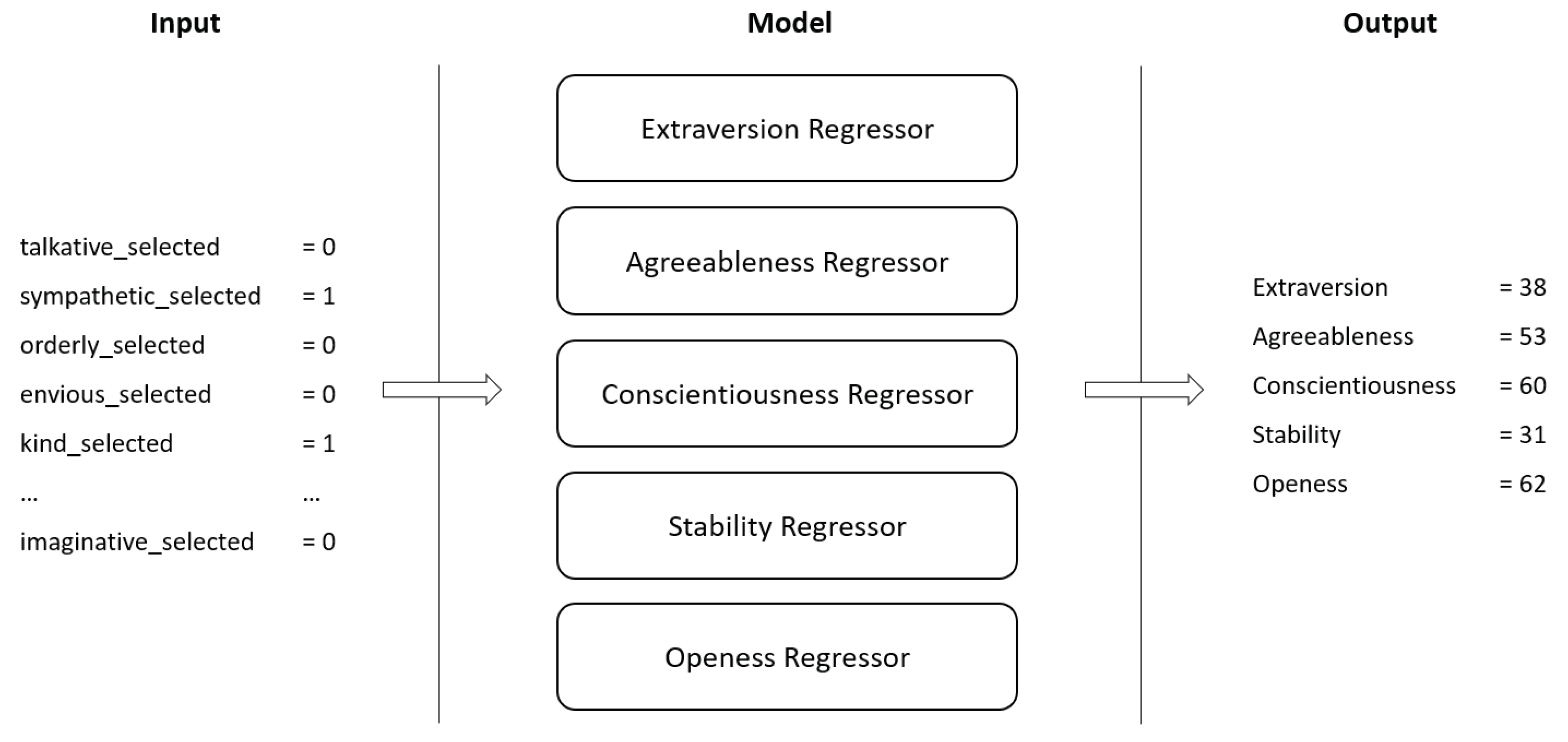
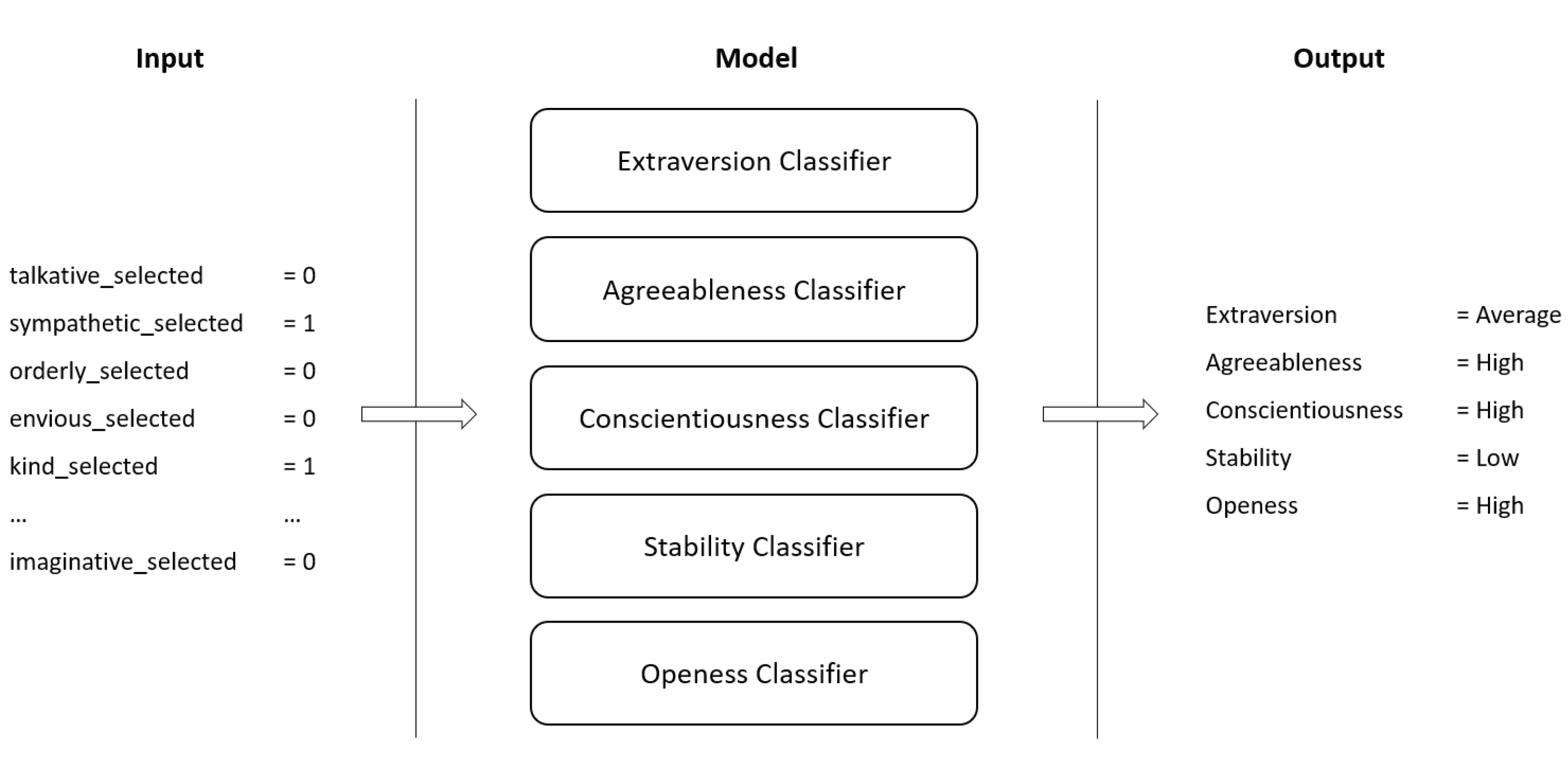
Two distinct ML architectures were experimented. One uses Gradient Boosted Trees regressors to obtain the exact value of each personality trait (Architecture I) while the other uses Gradient Boosted Trees classifiers to obtain the bin of each personality trait (Architecture II). Different experiments were conducted with two distinct datasets. One with 250 observations (No DA) and another with 5230 observations (With DA). Both architectures receive, as input, the one-hot encoded selection of adjectives.

Nested cross-validation was performed to tune the hyperparameters and to have a stronger validation of the obtained results. Inner cross-validation was performed using $k=4$, with random search being used to find the best set of hyperparameters. In the inner loop, 700 fits were performed (4 folds × 175 combinations). The outer cross-validation loop used $k=3$, totalling 2100 fits (3 folds × 700 fits). Two independent training trials were performed, with a grand total of 4200 fits (2 trials × 2100 fits) per architecture per dataset.

3.1. Architecture I—Big Five Regressors

All candidate models were evaluated in regard to RMSE and MAE error metrics.

Table 5. Architecture I results with and without data augmentation, for each independent trial, with RMSE as metric. Hyperparameters described by letters as follows: a. number of estimators, b. eta, c. gamma, d. trees’ max depth, e. minimum child weight and f. colsample by tree.

Trial	CV Split	Best Score	Evaluation	Fit Time (min)	a.	b.	c.	d.	e.	f.
No Data Augmentation
1	1	7.813	8.078	3.8	300	0.05	0.04	4	6	0.2
1	2	8.015	7.560	3.8	300	0.05	0.02	4	4	0.2
1	3	8.203	7.512	3.7	300	0.01	0.04	4	4	0.2
2	1	8.024	7.594	3.7	300	0.10	0.08	4	8	0.2
2	2	8.184	7.161	3.7	300	0.05	0.02	4	8	0.2
2	3	7.847	7.961	3.7	300	0.05	0.04	4	8	0.2
With Data Augmentation
1	1	5.692	5.464	64.8	300	0.10	0.02	12	4	0.3
1	2	5.604	5.602	65.9	300	0.01	0.02	18	4	0.3
1	3	5.646	5.520	69.6	300	0.01	0.02	18	4	0.3
2	1	5.637	5.537	68.4	300	0.01	0.02	12	4	0.3
2	2	5.632	5.482	65.7	300	0.01	0.04	18	6	0.3
2	3	5.673	5.467	67.4	300	0.01	0.08	12	4	0.3

depicts the best hyperparameter configuration for Architecture I, for both datasets. What immediately stands out is the better performance of the candidate models when using the larger dataset. In fact, RMSE decreases about 30% when using the dataset With DA. This was already expected since the dataset with No DA was made of only 250 observations.

Overall, for Architecture I with No DA the error is of approximately 8 units of measure. Since RMSE outputs an error in the same unit of the features that are being predicted by the model, it means that this Architecture is able to obtain the value of each personality trait with an error of 8 units. On the other hand, for Architecture I With DA, RMSE is of approximately 5.6 units of measure. It is also possible to discern that RMSE tends to be more stable when using the With DA dataset when compared to the No DA dataset which shows higher error variance. In Table 5, the Evaluation column presents the error value of the best candidate model in the outer test fold. These values provide a second and stronger validation of the ability to classify of the best model per split.

The hyperparameter tuning process is significantly faster for Architecture I with No DA, taking around 3.7 min to perform 700 fits and around 22 min to perform the full run. On the other hand, Architecture I With DA takes more than 1 hour to perform the same amount of fits, requiring more than 6.5 hours to complete. Overall, the models that behaved the best used 300 gradient boosted trees. Interestingly, when using the dataset with No DA, all models required 20% of the entire feature set when constructing each tree (colsample by tree) and used a maximum depth of 4 levels, building shallower trees which helps controlling overfitting in the smaller dataset. On the other hand, when using the dataset With DA, the best models not only required 30% of the feature set but also required deeper trees, which indicate the need for more complex trees to find relations in the larger dataset. To strengthen this assertion, the learning rate is also smaller in Architecture I With DA allowing models to move slower through the gradient.

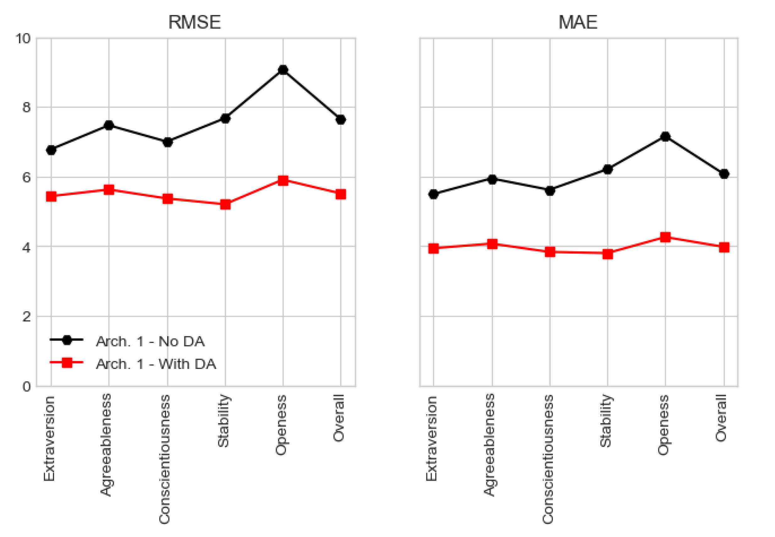
Focusing the results obtained from testing in the test fold of the outer-split, Architecture I With DA presents a global RMSE of 5.512 and MAE of 3.979. On the other hand, Architecture I with No DA presents higher error values, with a global RMSE and MAE of 7.644 and 6.082, respectively. The fact that RMSE and MAE have relatively close values implies that not many outliers, or distant classifications, were provided by the models. It is also interesting to note that, independently of the dataset, Openness is the most difficult trait to classify. All these data is given by

Table 6. Evaluation results of Architecture I, with and without data augmentation, obtained from the test folds of the outer-split.

Metric	Global	Extraversion	Agreeableness	Conscient.	Stability	Openness
No Data Augmentation
MAE	6.082	5.495	5.942	5.616	6.205	7.153
MSE	58.527	45.973	55.984	49.230	58.933	82.514
RMSE	7.644	6.778	7.468	7.000	7.668	9.061
With Data Augmentation
MAE	3.979	3.937	4.071	3.832	3.798	4.259
MSE	30.385	29.529	31.630	28.813	27.069	34.884
RMSE	5.512	5.433	5.623	5.367	5.201	5.906

, where the MSE is also displayed, being used to compute the RMSE.

Figure 7 provides a graphical view of RMSE and MAE for Architecture I for both datasets, being possible to discern that both metrics present a lower error value when conceiving models over the augmented dataset.

3.2. Architecture II—Big Five Bin Classifiers

Architecture II candidate models, which classify personality traits in three bins (low, average and high), were evaluated using several classification metrics.

Table 7. Architecture II results with and without data augmentation, for each independent trial, with sample accuracy as metric. Hyperparameters described by letters as follows: a. number of estimators, b. eta, c. gamma, d. trees’ max depth, e. minimum child weight and f. colsample by tree.

Trial	CV Split	Best Score	Evaluation	Fit Time (min)	a.	b.	c.	d.	e.	f.
No Data Augmentation
1	1	0.144	0.131	8.4	500	0.05	0.02	4	6	0.3
1	2	0.180	0.181	8.6	400	0.01	0.08	4	4	0.2
1	3	0.138	0.108	8.4	300	0.01	0.04	12	8	0.3
2	1	0.175	0.143	8.5	300	0.05	0.04	4	4	0.2
2	2	0.138	0.181	8.4	500	0.10	0.02	18	4	0.3
2	3	0.155	0.133	8.4	400	0.05	0.08	18	8	0.3
With Data Augmentation
1	1	0.458	0.486	128.6	300	0.10	0.02	12	4	0.3
1	2	0.464	0.466	130.1	300	0.01	0.08	12	4	0.3
1	3	0.453	0.468	133.6	400	0.10	0.08	12	4	0.2
2	1	0.465	0.490	129.4	300	0.10	0.02	18	4	0.3
2	2	0.466	0.466	123.6	300	0.01	0.04	12	4	0.3
2	3	0.448	0.480	125.3	500	0.10	0.08	18	4	0.2

depicts the best hyperparameter configuration for Architecture II, for the two datasets, using accuracy as metric. Again, models conceived over the dataset With DA outperform those conceived over the dataset with No DA, more than doubling the accuracy value. In addition, their evaluation values also tend to be more stable and less prone to variations. However, one may argue that the accuracy values attained by the candidate models and presented in Table 7 are low. Hence, it is of the utmost importance to assert that such accuracy values correspond to samples that had all five traits correctly classified. I.e., if one trait of a sample was wrongly classified, than that sample would be considered as badly-classified even if the remaining four traits were correctly classified. To provide a stronger validation metric,

Table 8. Evaluation results of Architecture II, with and without data augmentation, based on trait’s accuracy and obtained from the test folds of the outer-split.

Metric	Global	Extraversion	Agreeableness	Conscient.	Stability	Openness
No Data Augmentation
Mean Error	0.338	-	-	-	-	-
Micro F1-Score	0.663	0.728	0.660	0.620	0.648	0.656
Macro F1-Score	0.459	0.532	0.462	0.419	0.443	0.438
Macro Precision	0.477	0.590	0.468	0.413	0.445	0.468
Macro Recall	0.464	0.525	0.469	0.434	0.447	0.447
With Data Augmentation
Mean Error	0.165	-	-	-	-	-
Micro F1-Score	0.835	0.846	0.834	0.831	0.843	0.822
Macro F1-Score	0.776	0.770	0.795	0.801	0.731	0.782
Macro Precision	0.830	0.826	0.854	0.840	0.809	0.819
Macro Recall	0.742	0.731	0.758	0.774	0.691	0.755

provides metrics based on traits’ accuracy instead of samples’ accuracy, presenting significantly higher values.

Still regarding Table 7, it becomes clear that the tuning process is significantly faster for Architecture II with No DA, taking around 50 min to complete the process. On the other hand, when using the larger dataset, the process takes more than 12 hours to complete. Overall, models tend to use 300 gradient boosted trees and require 30% of the entire feature set per tree. The best classifiers also require deeper trees, with 12 or 18 levels. It is also worth mentioning that all the best models conceived over the dataset With DA required a minimum child weight of 4. This hyperparameter defines the minimum sum of weights of all observations required in a child node, being used to control overfitting and prevent under-fitting, which may happen if high values are used when setting this hyperparameter.

As stated previously, all metrics provided in Table 8 are based on traits’ accuracy. Using class accuracy instead of sample accuracy, the mean error of Architecture II candidate models using the dataset With DA is of 0.165, which corresponds to an accuracy higher than 83%. On the other hand, the mean error with No DA increases to 0.338. Overall, all models show better results when using the dataset With DA.

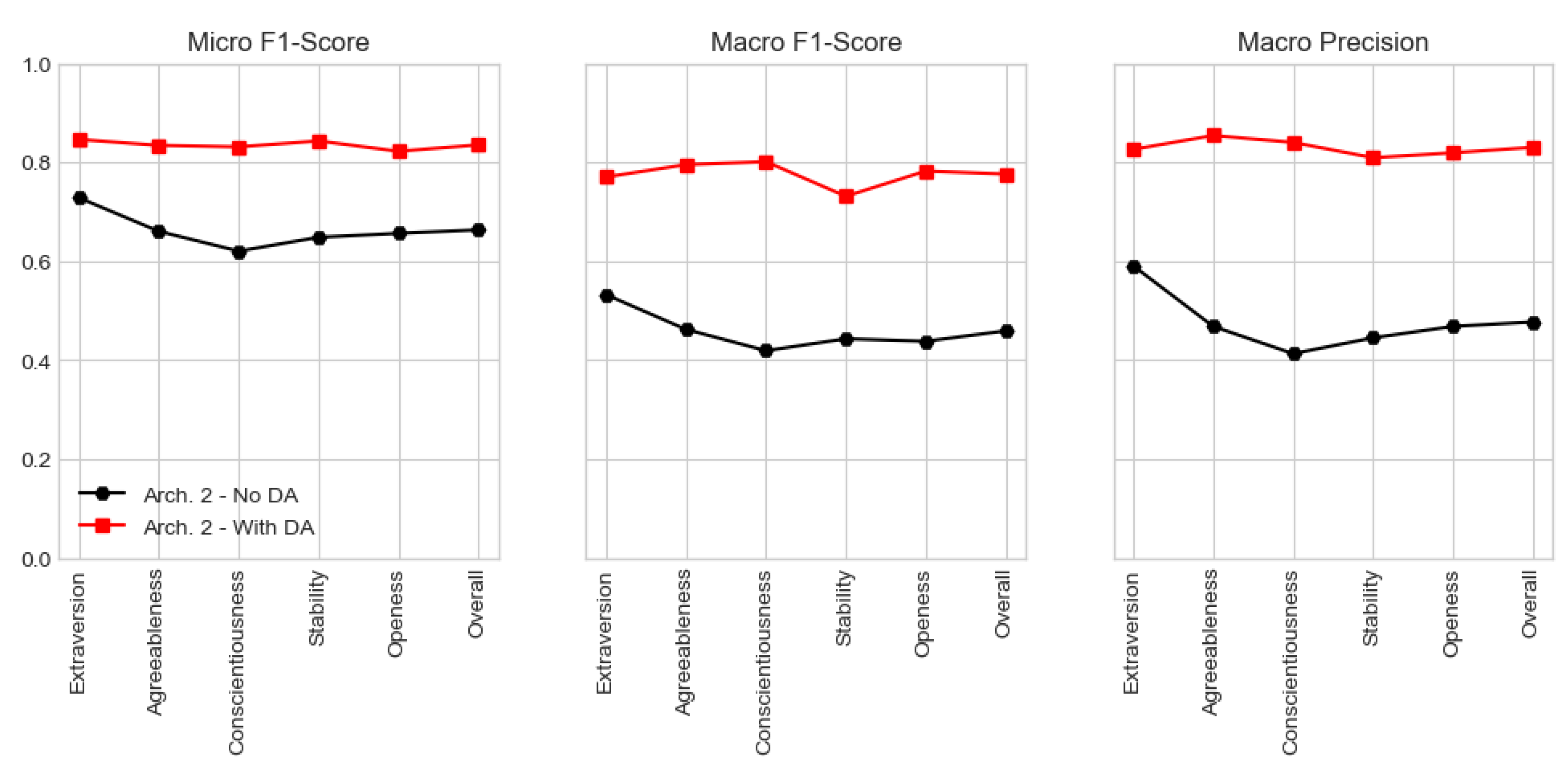
In this study, both micro and macro-averaged metrics were evaluated. However, since we are interested in maximising the number of correct predictions each classifier makes, special importance is given to micro-averaging. In fact, micro f1-score of the classifiers conceived over the dataset With DA display an interesting overall value of 0.835, with the Openness trait being, again, the one showing the lower value. It is worth mentioning that micro-averaging in a multi-class setting with all labels included, produces the same exact value for the f1-score, precision and recall metrics, being this the reason why Table 8 only displays micro f1-score. On the other hand, macro-averaging computes each error metric independently for each class and then averages the metrics, treating all classes equally. Hence, since models depict a lower macro f1-score when compared to the micro one, this could mean that there may be some classes that are less used when classifying, such as low or high. Nonetheless, macro f1-score still present a very interesting global value of 0.776. Macro-averaged precision also depicts a high value, strengthening the ability of models to correctly classify true positives and avoid false positives. Finally, models’ global macro-averaged recall is of 0.742, still a significant value that tells us that the best candidate models are able, in some extent, to avoid false negatives.

Figure 8 provides a graphical view of micro and macro-averaged f1-score and precision for Architecture II for both datasets, being again possible to recognise a better performance when using the dataset With DA.

3.3. Feature Importance

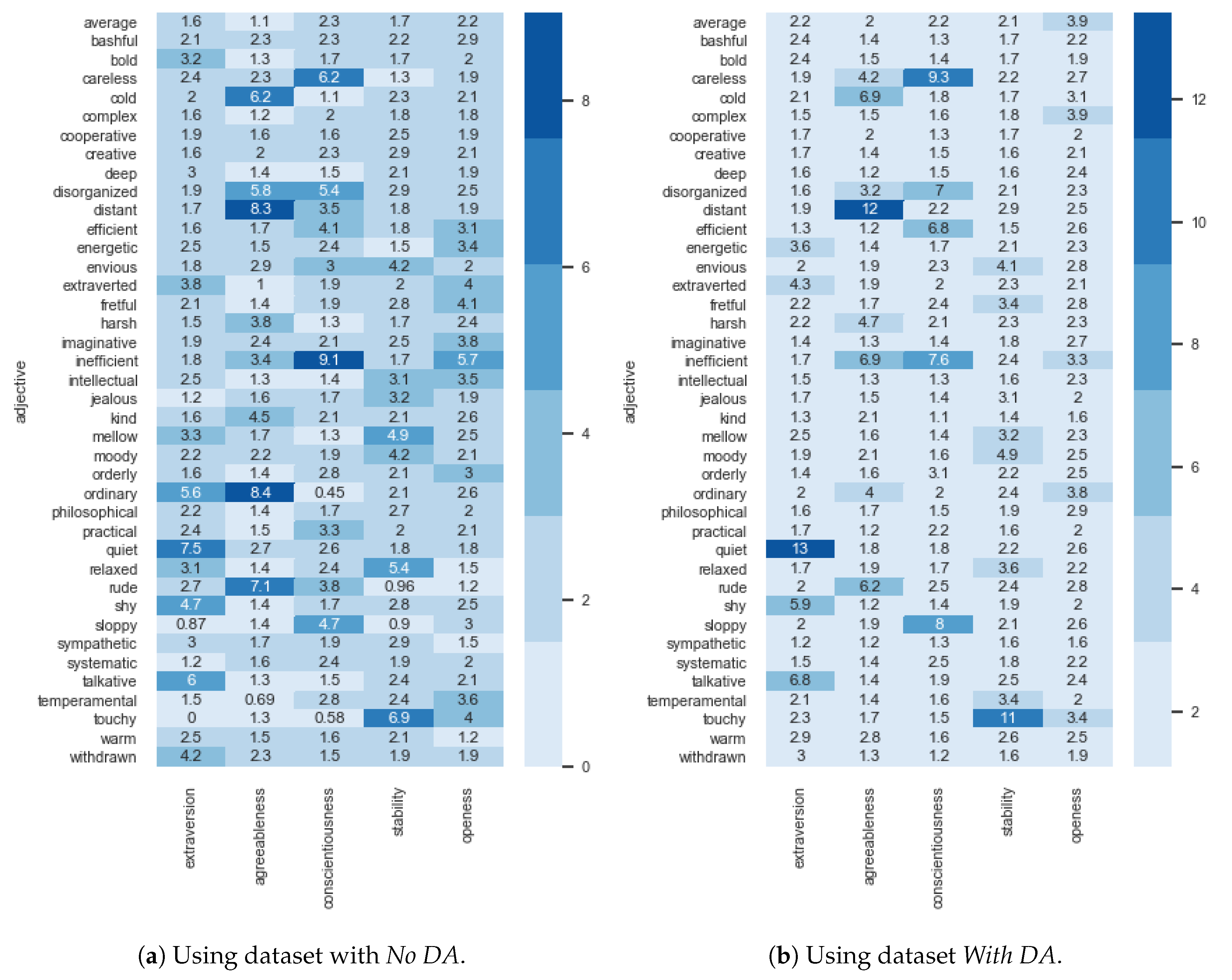
Gradient Boosted Trees allow the possibility of estimating feature importance, i.e., a score that measures how useful each feature was when building the boosted trees. This importance was estimated using gain as importance type, which corresponds to the improvement in accuracy brought by a feature to the branches it is on. A higher value for a feature when compared to another, implies it is more important for classifying the label.

Figure 9 presents the estimated feature importance of Architecture I using an heat-map view. Interestingly, models conceived using the dataset with No DA (Figure 9a) give an higher importance to the selection of the adjective inefficient when classifying the Conscientiousness trait. Sloppy, disorganized and careless are other adjectives that assume special relevance when classifying the same personality trait. Regarding the Extraversion trait, talkative, quiet and withdrawn are the most important adjectives, being only then followed by the extroverted and energetic ones. The Agreeableness trait gives higher importance to distant, harsh, cold and rude. On the other hand, feature importance is more uniform in the Stability and Openness personality traits, with the most important adjectives assuming a relative importance of about 7%. Another interesting fact that arises from these results, is that some adjectives have lower importance for all five traits. Examples include bashful, bold, intellectual and jealous.

As for the models conceived using the dataset With DA (Figure 9b), results are similar to the smaller dataset. In these models there are less important features, but the ones considered as important have a stronger importance. An example is the case of the adjective talkative for the Extraversion trait, which increases its importance from 16% to 22%, and quiet, which increases from 11% to 17%. Withdrawn and quiet have a reduced importance. Interestingly, for the Agreeableness trait, the adjective kind becomes the most important one, increasing from 3.2% to 15%. The Openness trait still assumes a more uniform importance for all features, being this one of the reasons why it was the trait showing worst performance using Architecture I models.

Regarding Architecture II, Figure 10 presents the estimated feature importance for both datasets. What immediately draws one attention is the fact that importance values are much more balanced when compared to Architecture I. Indeed, the highest importance value is of 9.1% with No DA and 13% With DA when compared to 20% and 22% of Architecture I, respectively. Nonetheless, except for a few exceptions, adjectives assuming higher importance in Architecture I also assume higher importance in Architecture II. The main difference is that values are closer together, having a lower amplitude.

4. Discussion and Conclusions

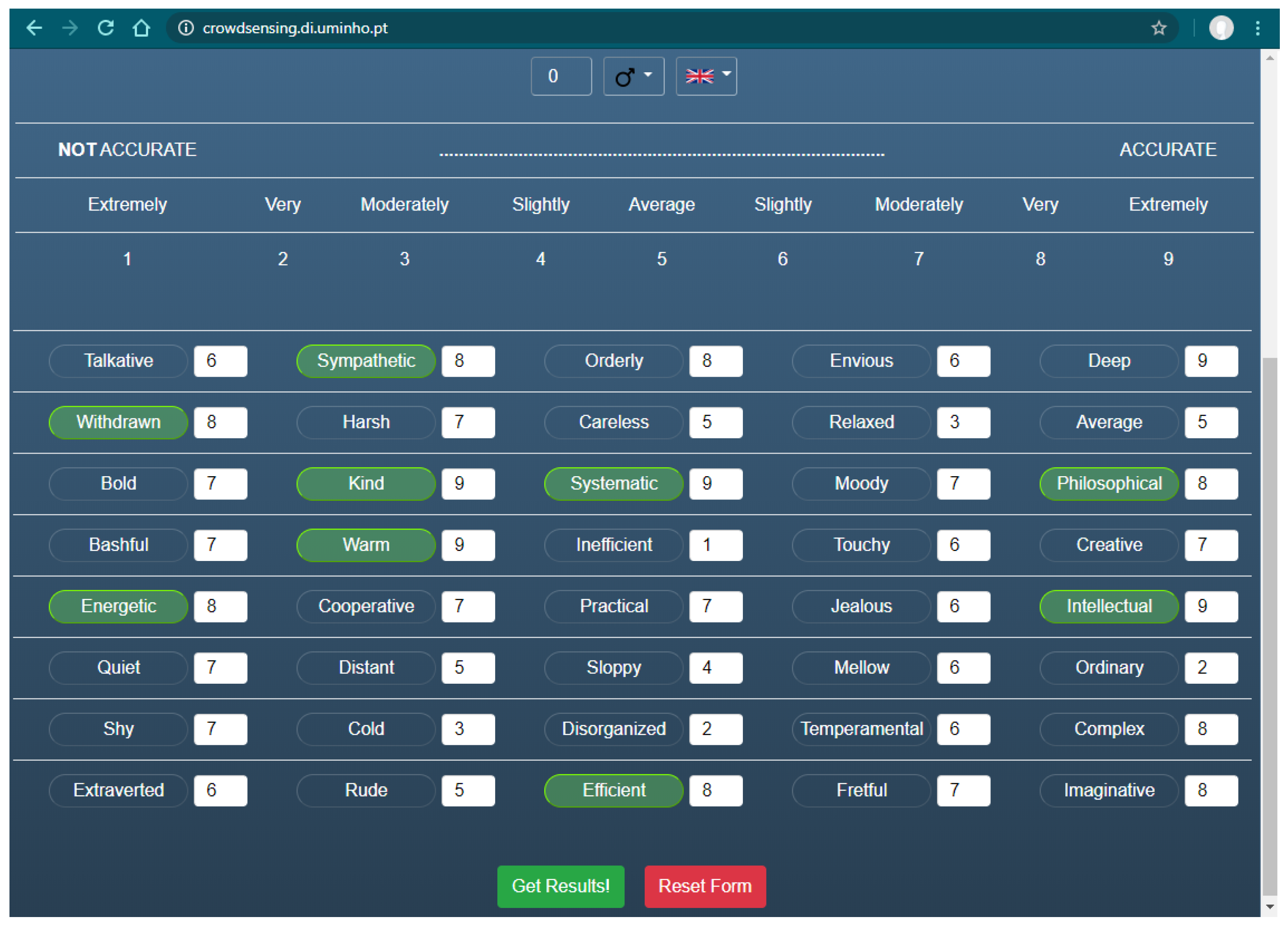
The proposed ASAP method aims to use ML-based models to reinstate the process of rating adjectives or answering questions by an adjective selection process. To achieve this goal, two different ML architectures were proposed, experimented and evaluated. The first architecture uses Gradient Boosted Trees regressors to quantify the Big Five personality traits. Overall, this architecture is able to quantify such traits with an error of approximately 5.5 units of measure, providing an accurate output given the limited amount of available records. On the other hand, Architecture II uses Gradient Boosted Trees classifiers to qualify the bin in which the subject stands, for each trait. Bins are based on Saucier’s original study where trait scores between $[8,29]$ are considered Low, between $[30,50]$ are considered Average, and between $[51,72]$ are considered High. This architecture was able to quantify the personality traits with a micro-averaged f1-score of more than 83%. A better performance of both architectures in the augmented dataset was also expected since the original dataset had a limited amount of records. The implemented data augmentation techniques aimed to increase the dataset size following well-defined rationales but also included several randomised decisions based on a probabilistic approach in order to reduce bias and create a more generalised version of the dataset. For this, data exploration and pattern mining, in the form of Association Rules Learning, assumed an increased importance, allowing us to understand relations between selected adjectives. Results for records with very few adjectives selected may be biased to the dataset used to train the models since the ability to quantify traits based on the selection of just one or two adjectives is of an extreme difficulty. Hence, for the ASAP method to behave properly, subjects should be encouraged to select four, or more, adjectives.

A further validation was carried out by means of a significance analysis between the correlation differences of predicted and actual scores. The best overall candidate model of Architecture I was trained using, as input data, 90% of the original dataset, with the remaining being used to obtain predictions. Predictions were compared with the actual scores of the five traits. As expected, the p-value returned an high value (0.968), with a z-score of 0.039. Such values tell, with a high degree of confidence, that the null hypothesis should be retained and that both correlation coefficients are not significantly different from each other. This is in line with expectations since the conceived models are optimizing a differentiable loss function, using a gradient descent procedure that reduces the model’s loss to increase the correlation between predictions and actual scores.

Architecture II took significantly more time to fit than Architecture I. However, it provides more accurate results, which are less prone to error. It should be noted that Architecture II only provides an approximation to the Big Five of the subject, i.e., it does not numerically quantify each trait, instead it tells in which bin the subject finds himself. This can be useful in cases where the general qualification of each trait is more important than the specific score of the trait. On the other hand, Architecture I will provide an exact score for each personality trait based on a selection of adjectives. Indeed, the working hypothesis has been confirmed, i.e., it is possible to achieve promising performances using ML-based models where the subject, instead of rating forty adjectives or answering long questions, selects the adjectives he relates the most with. This allows one to obtain the Big Five using a method with a reduced complexity and that takes a small amount of time to complete. Obviously, the obtained results are just estimates, with an underlying error. The conducted experiments shown the ability of ML-based models to compute estimates of personality traits, and should not be seen as a definitive psychological assessment of one’s personality traits. For a full personality assessment, tests such as the one proposed by Saucier, Goldberg or the NEO-personality-inventory should be used.

The use of augmented sets of data may bring an intrinsic bias to the candidate models. In all cases, preference should always be given to the collection and use of real data. However, in scenarios where data is extremely costly, an approximation may allow ML models to be analyzed with augmented data. In such scenarios, data augmentation processes should make use of several randomized decisions based on probabilistic approaches to create a generalized version of the smaller dataset. Experiments should be carefully conducted, implementing two, or more, independent trials, cross-validation and even nested cross-validation. Models, when deployed, should monitor their performance and, in situations with a clear performance degradation, should be re-trained with new collected data.

In Saucier’s test, each personality trait is computed using the rating of eight unipolar adjectives, i.e, no adjective is used for more than one personality trait. Indeed, it is known, beforehand, which adjectives are used by each trait. For example, the Extroversion trait is computed based on four positively weighted adjectives (extroverted, talkative, energetic and bold) and four negative ones (shy, quiet, withdrawn and bashful). However, in the proposed ML architectures that make the ASAP method, all 40 adjectives are used to compute all traits, allowing the ML models to use adjectives selection/non-selection to compute several traits, thus harnessing inter-trait relationships. For instance, bold, one of the adjectives used by Saucier to compute Extroversion, shows a small importance in the conceived architectures when quantifying Extroversion. The same happens for bashful in Extroversion, creative in Openness, and practical in Conscientiousness, just to point a few. This could lead us to hypothesise that, one, the list of forty adjectives could be further reduced to a smaller set of adjectives by removing those that are shown to have a smaller importance and that, two, there are adjectives that can be used to quantify distinct personality traits, such as the case of disorganised, which can be used for the Conscientiousness and the Agreeableness traits. It is also interesting to note the lack of features assuming high importance when quantifying Openness. In fact, one of its adjectives, ordinary, seems to assume higher importance in the Agreeableness trait. Overall, Saucier’s adjective-trait relations are being found and used by the conceived models.

Since the conceived ML architectures proved to be both performant and efficient using a selection of adjectives, future research points towards a reduction to the minimum required set of adjectives that does not harm the method’s accuracy, further reducing complexity and the time it takes to be performed by the subject.

References

1. Barlett, C.; Anderson, C. Direct and indirect relations between the Big 5 personality traits and aggressive and violent behavior. Personal. Individ. Differ. 2012, 52, 870–875. [Google Scholar] [CrossRef]
2. Rothmann, S.; Coetzer, E.P. The big five personality dimensions and job performance. J. Ind. Psychol. 2003, 29. [Google Scholar] [CrossRef] [Green Version]
3. Orzeck, T.; Lung, E. Big-five personality differences of cheaters and non-cheaters. Curr. Psychol. 2005, 24, 274–286. [Google Scholar] [CrossRef]
4. Kazdin, A. Encyclopedia of Psychology; American Psychological Association: Washington, DC, USA, 2000; Volume 3. [Google Scholar]
5. Salgado, J. Big Five Personality Dimensions and Job Performance in Army and Civil Occupations: A European Perspective. Hum. Perform. 1998, 11, 271–288. [Google Scholar]
6. Ashton, M.; Lee, K. The HEXACO–60: A Short Measure of the Major Dimensions of Personality. J. Personal. Assess. 2009, 91, 340–345. [Google Scholar] [CrossRef] [PubMed]
7. Myers, I. The Myers-Briggs Type Indicator: Manual (1962); Consulting Psychologists Press: Palo Alto, CA, USA, 1962. [Google Scholar] [CrossRef]
8. Riso, D.; Hudson, R. Understanding the Enneagram: The Practical Guide to Personality Types; Houghton Mifflin Harcourt: Boston, MA, USA, 2000. [Google Scholar]
9. Costa, P., Jr.; McCrae, R. Domains and facets: Hierarchical personality assessment using the Revised NEO Personality Inventory. J. Personal. Assess. 1995, 64, 21–50. [Google Scholar] [CrossRef] [PubMed] [Green Version]
10. Goldberg, R. The development of markers for the Big-Five factor structure. Psychol. Assess. 1992, 4, 26. [Google Scholar] [CrossRef]
11. John, O.; Srivastava, S. The Big Five trait taxonomy: History, measurement, and theoretical perspectives. In Handbook of Personality: Theory and Research; Guilford Publications: New York, NY, USA, 1999; Volume 2, pp. 102–138. [Google Scholar]
12. Kosinski, M.; Bachrach, Y.; Kohli, P.; Stillwell, D.; Graepel, T. Manifestations of user personality in website choice and behaviour on online social networks. Mach. Learn. 2014, 95, 357–380. [Google Scholar] [CrossRef] [Green Version]
13. Saucier, G. Mini-Markers: A brief version of Goldberg’s unipolar Big-Five markers. J. Personal. Assess. 1994, 63, 506–516. [Google Scholar] [CrossRef] [PubMed]
14. Majumder, N.; Poria, S.; Gelbukh, A.; Cambria, E. Deep Learning-Based Document Modeling for Personality Detection from Text. IEEE Intell. Syst. 2017, 32, 74–79. [Google Scholar] [CrossRef]
15. Yu, J.; Markov, K. Deep learning based personality recognition from Facebook status updates. In Proceedings of the IEEE 8th International Conference on Awareness Science and Technology (iCAST), Taichung, Taiwan, 8 November 2017; pp. 383–387. [Google Scholar] [CrossRef]
16. Sumner, C.; Byers, A.; Boochever, R.; Park, G. Predicting Dark Triad Personality Traits from Twitter Usage and a Linguistic Analysis of Tweets. In Proceedings of the 11th International Conference on Machine Learning and Applications, Boca Raton, FL, USA, 12–15 December 2012; Volume 2, pp. 386–393. [Google Scholar] [CrossRef]
17. Pennebaker, J.; King, A. Linguistic styles: Language use as an individual difference. J. Personal. Soc. Psychol. 1999, 77, 1296–1312. [Google Scholar] [CrossRef]
18. Park, G.; Schwartz, H.; Eichstaedt, J.; Kern, M.; Kosinski, M.; Stillwell, D.; Ungar, L.; Seligman, M. Automatic personality assessment through social media language. J. Personal. Soc. Psychol. 2015, 108, 934–952. [Google Scholar] [CrossRef] [PubMed] [Green Version]
19. Schwartz, H.; Eichstaedt, J.; Kern, M.; Dziurzynski, L.; Ramones, S.; Agrawal, M.; Shah, A.; Kosinski, M.; Stillwell, D.; Seligman, M.; et al. Personality, Gender, and Age in the Language of Social Media: The Open-Vocabulary Approach. PLoS ONE 2013, 8. [Google Scholar] [CrossRef] [PubMed]
20. Cerasa, A.; Lofaro, D.; Cavedini, P.; Martino, I.; Bruni, A.; Sarica, A.; Mauro, D.; Merante, G.; Rossomanno, I.; Rizzuto, M.; et al. Personality biomarkers of pathological gambling: A machine learning study. J. Neurosci. Methods 2018, 294, 7–14. [Google Scholar] [CrossRef] [PubMed]
21. Mehta, Y.; Majumder, N.; Gelbukh, A.; Cambria, E. Recent trends in deep learning based personality detection. Artif. Intell. Rev. 2019. [Google Scholar] [CrossRef] [Green Version]
22. Levitan, S.; Levitan, Y.; An, G.; Levine, M.; Levitan, R.; Rosenberg, A.; Hirschberg, J. Identifying Individual Differences in Gender, Ethnicity, and Personality from Dialogue for Deception Detection. In Proceedings of the Second Workshop on Computational Approaches to Deception Detection, San Diego, CA, USA, 17 June 2016; pp. 40–44. [Google Scholar] [CrossRef] [Green Version]
23. Levitan, S.; Levine, M.; Hirschberg, J.; Cestero, N.; An, G.; Rosenberg, A. Individual Differences in Deception and Deception Detection. Available online: Https://Www.Semanticscholar.Org/Paper/Individual-Differences-In-Deception-And-Deception-Levitan-Levine/295332ebfb77387f4ccbacbd214edf72caf3e331 (accessed on 3 March 2020).
24. Gurpinar, F.; Kaya, H.; Salah, A. Combining Deep Facial and Ambient Features for First Impression Estimation. In Proceedings of the Computer Vision—ECCV 2016 Workshops, Amsterdam, The Netherlands, 11–14 October 2016; Volume 9915. [Google Scholar] [CrossRef]
25. Güçlütürk, Y.; Güçlü, U.; Pérez, M.; Escalante, H.; Baró, X.; Andujar, C.; Guyon, I.; Junior, J.; Madadi, M.; Escalera, S.; et al. Visualizing Apparent Personality Analysis with Deep Residual Networks. In Proceedings of the IEEE International Conference on Computer Vision Workshops (ICCVW), Venice, Italy, 22–29 October 2017; pp. 3101–3109. [Google Scholar] [CrossRef] [Green Version]
26. Zhang, C.; Zhang, H.; Wei, X.; Wu, J. Deep Bimodal Regression for Apparent Personality Analysis. In Proceedings of the Computer Vision—ECCV 2016 Workshops, Amsterdam, The Netherlands, 11–14 October 2016; Volume 9915. [Google Scholar] [CrossRef]
27. Wessa, P. Cronbach alpha (v1.0.5) in Free Statistics Software (v1.2.1). Available online: https://www.wessa.net/rwasp_cronbach.wasp/ (accessed on 1 May 2020).
28. Friedman, J. Greedy Function Approximation: A Gradient Boosting Machine. Ann. Stat. 2001, 29, 1189–1232. [Google Scholar] [CrossRef]
29. Cawley, G.; Talbot, N. On Over-fitting in Model Selection and Subsequent Selection Bias in Performance Evaluation. J. Mach. Learn. Res. 2010, 11, 2079–2107. [Google Scholar]
30. Yu, W.; Na, Z.; Fengxia, Y.; Yanping, G. Magnetic resonance imaging study of gray matter in schizophrenia based on XGBoost. J. Integr. Neurosci. 2018, 17, 331–336. [Google Scholar] [CrossRef]
31. Sahoo, D.; Balabantaray, R. Single-Sentence Compression using XGBoost. Int. J. Inf. Retr. Res. 2019, 9, 11. [Google Scholar] [CrossRef] [Green Version]
32. Pesantez-Narvaez, J.; Guillen, M.; Alcañiz, M. Predicting Motor Insurance Claims Using Telematics Data — XGBoost versus Logistic Regression. Risks 2019, 7, 16. [Google Scholar] [CrossRef] [Green Version]
Figure 1. Platform for data collection allowing the subject to perform Saucier’s Mini-Marker test and, at the same time, select a set of adjectives that describe him the most.
Processes 08 00618 g001
Figure 2. Number of times each adjective was selected.
Processes 08 00618 g002
Figure 3. Mean rating values to set an adjective as selected.
Processes 08 00618 g003
Figure 4. Distribution of observations per bin and personality trait.
Processes 08 00618 g004
Figure 5. Architecture I—Big Five regressors.
Processes 08 00618 g005
Figure 6. Architecture II—Big Five bin classifiers.
Processes 08 00618 g006
Figure 7. Graphical view of Architecture’s I RMSE and MAE for both datasets.
Processes 08 00618 g007
Figure 8. Graphical view of Architecture’s II micro and macro-averaged f1-score and precision for both datasets.
Processes 08 00618 g008
Figure 9. Feature importance heat-map of Architecture I.
Processes 08 00618 g009
Figure 10. Feature importance heat-map of Architecture II.
Processes 08 00618 g010