Abstract
Bearings are essential components in rotating machines. They ensure the rotation and power transmission. So, these components are essential elements for industrial machines. Thus, real-time monitoring is required to detect a possible anomaly, diagnose the failure of rolling bearing and follow its evolution. This paper presents a methodology for automatic online implementation of fault diagnosis of rolling bearings, by AOC-OPTICS (automatic online classification monitoring based on ordering points to identify clustering structure, OPTICS). The algorithm consists of three phases namely: initialization, detection and follow-up. These phases use the combination of features extraction methods, smart ranking, features weighting and classification by the OPTICS method. Two methods have been integrated in the dimension reduction step to improve the efficiency of detection and the followed of the defect (relief method and t-distributed stochastic neighbor embedding method). Thus, the determination of the internal parameters of the OPTICS method is improved. A regression model and exponential model are used to track the fault. The analytical simulations discuss the influence of parameters automation. Experimental validation shows detection with 100% accuracy and regression models of monitoring reaching .
1. Introduction
The automation of techniques takes place around the world in the manufacturing and processing of industrial sectors [1,2]. In the industrial and rotary machines, the main idea of automation is the monitoring without input parameters. The error is human, and the limitation of inexact input parameters affects the accuracy of monitoring, so it was interesting to make an autonomous method. There is a growing demand for real-time monitoring in the rotary machines to facilitate advanced maintenance programs [3]. Rotary machines are most often made of a significant and critical component: the rolling bearings [4].
The monitoring of rolling bearings gets the scientist’s attention; so many methods applied to detect defects such as support vector machine [5], Bayesian network [6] and clustering [7]. Numerous literature reviews are available on monitoring methods [8,9]. From all these used methods, clustering analysis is one of the most remarkable approaches [10,11,12]. The density-based method is one of them, the clusters of dense regions of data separated from the less dense [11]. The method OPTICS (ordering points to identify clustering structure), subdivided from density-based, has the basic idea to separate clusters by density [13]. In addition, it has the advantage to attain clusters with varied data density. Clustering by OPTICS methods is an unsupervised learning method directly implemented to vibration data. Being thus can be applied directly in the industrial environments without trained by data measured on a machine under a fault condition [7]. Further advantages of the method are its ease of programming and the accomplishment of a good trade-off and achieved the best performances. In addition, it is fast for small data, used with different density to detect and attain arbitrary and sphere-shaped clusters [14].
Within the framework of bearing monitoring, the OPTICS method integrated dynamic classification processes for real-time monitoring [15]. The algorithm proposes to make a detection of faults from two time features (rms and kurtosis). The monitoring is then carried out using three geometric values, the contour, the distance and the density. However, the process was incomplete and not completely automated, which required an expert.
The extracted features play an essential role in the classification, for that many methods used to eliminate unwanted and unimportant features. The relief method is used to select features for the classification of biomedical data. It eliminates the irrelevant features and to prepare data of rolling bearings for the classification [16]. The Chi-square is another method that has the same aim of the relief to reduce and rank features, this method used ranking features to detect the defect in the rolling bearing [17]. After selecting features and reducing them by eliminating the uncorrelated ones, the importance of dimension reduction comes before starting the classification. In the literature, many methods have applied for dimension reduction, principal component analysis (PCA) [18] and kernel principal component analysis (KPCA) [19], to detect the defect in rolling bearings. A recently developed nonlinear dimensionality reduction technique shows its efficiency in the detection of a fault in rotary based on t-distributed stochastic neighbor embedding (t-SNE) [20].
The parameters specific to OPTICS are also subject to automation. The lack of automation concerns the choice of features according to a library and the internal parameters of OPTICS: (cluster radius), (the minimum number of data points needed to cluster) and the distance metric used to calculate instances between arrays [15]. The determination of the parameter values of the OPTICS algorithm can be a challenging task because the parameter values affect the accuracy and precision of the clustering. Many researchers have discussed this topic, and they were looking for ways to solve it. An automated algorithm AE-DBSCAN, proposed by [21], defines like the K-nearest neighbor for this . Regarding the choice of distance, [22] show the hardness approximation of data with Euclidean distance in k-means clustering. Manhattan outperforms the Euclidean distance with the k-means method. The aim is to automate calculation of all the parameters and to offer a complete real-time monitoring solution dedicated to the bearings.
This paper proposes an Online One Class Monitoring based on OPTICS Classification for Rolling Bearing, automatic online classification monitoring based on ordering points to identify clustering structure (AOC-OPTICS). The input parameters are limited to the initialization time of the method and the number of signals collected at a monitoring time t. It integrates the detection and monitoring of the evolution of a fault. After an initialization phase, the detection is carried out by a multidimensional analysis with extraction, ranking (relief method) selection (t-SNE) and classification (OPTICS) of one class clustering type. The follow-up is carried out when creating a new class. In this phase, geometric parameters from this class are proposed and discussed due to regressions models.
This paper is organized as follows. Section 1 introduces the context of the monitoring of the rotating elements and presents the bibliographical review on the contributions and the limits of the classification methods. Section 2 describes the OPTICS method and highlights the parameters to be automated. Section 3 presents the general methodology for automatic monitoring and follow-up of the healthy state of a bearing. Section 4 assesses the relevance of the methodology on data simulating the initiation and growth of a defect on the outer ring of a bearing. The automated parameters and their influences are discussed. Tracking parameters are defined, and mathematical laws are established. Section 5 corresponds to an experimental validation on a test bench. Section 6 concludes this study.
2. Classification Method OPTICS
OPTICS (ordering points to identify clustering structure) is a hierarchical clustering algorithm that relies on a density notion [13]. The application of this method is not limited to one field. It used in many fields and areas of biology, astronomy, topology, and recently for the detection of the defect in rolling bearings in rotary machines [15]. This method is capable of regrouping the base of data into an order of points with different parameter settings, and then detecting a meaningful difference of data with varied density by producing a request of data that is spatially closed to each other and can become a neighbor. It can separate considerable objects from noise and identify all possible levels of clusters. The main idea for the OPTICS algorithm is that for each point of a cluster the neighborhood of a given radius () has to contain at least a minimum number of points (), where ε and are input parameters. The concept of OPTICS algorithm starts by adding points to the clustered data in arbitrary shape and then to continue by adding points iteratively for developing the final cluster. The addition of points close to each other respecting the -neighbor order continues until getting the entire group.
The two-components of OPTICS are the core distance, and the reachability distance, , Equations (1) and (2). If the number of points in the vicinity of an object, , is less than , is the distance from p to its neighbour, In this case, is a core-object. The reachability distance of an object , , is the maximum of the Core Distance of p and the Euclidean distance between o and p. Figure 1a is a representation of the reachability distance and the core distance objects.
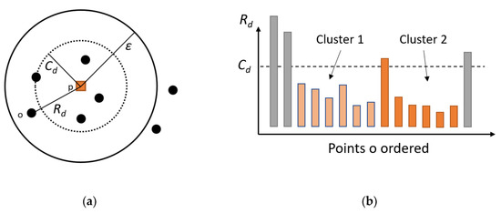
Figure 1.
(a) Representation of the core distance and reachability distance for . (b) Reachability plot.
The number of classes is determined from the reachability plot, Figure 1b. It corresponds to the number of valleys of the graphic representation as a function of the points o ordered.
3. Method
3.1. Global Architecture
The AOC-OPTICS method is developed for monitoring the state of health of a bearing throughout its entire life. It is based on the physical manifestations involved in the deterioration of a bearing. Thus 3 automated phases were proposed, Figure 2. Phase 1 considers that when a bearing is fitted, it is healthy during an interval . This phase allows the initialization of the method. Phase 2 corresponds to the failure detection phase. It is effective if the failure is not detected. Data agglomeration is used for early and reliable fault detection. The third phase corresponds to the follow-up of the evolution of the fault. In view of the evolutionary nature of the fault, the third phase is a follow-up loop of this state by second class geometrical values. It runs until the bearing fails. Each phase is described in the following sections and Table 1 shows the associated pseudo code.
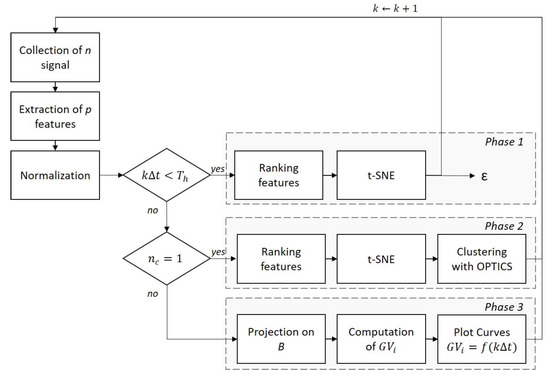
Figure 2.
Flowchart of AOC-OPTICS.

Table 1.
Pseudocode for automatic online classification monitoring based on ordering points to identify clustering structure (AOC-OPTICS).
3.2. Phase 1, Initialization
The first phase is executed for a duration , which is assumed to be a healthy phase of the bearing. For every iteration , signals were collected. features were extracted in the time, spectral and/or time-frequency domains. The use of a multidomain feature in the detection of defect bearing can offer an efficacy diagnosis for different defects of rolling bearings, with variated speed and load. The time domain provides nine characteristic features as descriptive statistics. The statistical indicators are widely used to their relations with significant bearing damages [23]. The frequency-domain allows one to localize and detect the nature of the bearing defect [24]. Six indicators are computed. The time scale domain uses the wavelet method to extract two features [25], Table 2. These indicators are stored in a matrix where each column corresponds to a signal and each row to an indicator.
Table 2.
Computed features. is the sequence of samples obtained after digitizing the time domain signals, is a signals series for i = 1, 2..., N. corresponds to the spectral density of the max coefficients of the continuous wavelet transform. is a spectrum for , is the number of spectrum lines, is the frequency value of the kth spectrum value.
At the time the indicator matrix is normalized , Equation (3). Normalization aims to transform the computed to be on a similar scale.
A ranking step is applied. The ranking features are a significant method for eliminating the unimportant features before reduction the dimension. The massive amount of data calculates features take a long time. To reduce this long process, the method of ranking features is implemented to minimize the number of features, which can make the calculation faster, without touching the accuracy of detecting the defect. For the AOC-OPTICS, two methods are compared in Section 4.3 to eliminate the unnecessary features, with the different amounts of features: the relief method and the chi-square method [26].
Although the nuisance of dimensionality poses serious problems, processing data with high dimensions has an advantage that the data can give more information. The reduction method t-distributed stochastic neighbor embedding (t-SNE) is a powerful dimensional reduction tool, which can reduce functionality dimensions and increase the recognition rate to an overwhelming majority. The dimension reduced to be in three components, which will give more accuracy than two dimensions. The difference accuracy between the dimensions noticed in the representation of amplitude. Due to the use of the three-component in this paper, figures are shown in three dimensions.
Finally, the calculation of is done after a reduction in dimension. corresponds to the maximum distance between the center of the class, and the neighbor, Equation (4).
The resulting class is a so-called healthy class, noted with center . This class corresponds to a reference state.
3.3. Phase 2, Detection
The second phase is a step to detect the mechanical failure. The objective of this phase is to detect a new state called the defective class, noted . At each new iteration , the indicators are extracted, normalized, sorted and reduced as in the previous phase. These features are tested by the OPTICS method to detect or not a second class. If only one class is obtained, which corresponds to the reference state, the algorithm remains in the detection phase, this new data feeds the reference state. If two classes are detected, this new class is obtained in a plan , which will be kept for the follow-up phase.
3.4. Phase 3, Follow-up
The third step is carried out in plan , which is determined in the previous phase. It is important to keep the same plan in order to visualize the evolution of the characteristics. This plan is the best plan to follow the evolution of the bearing failure. With each new series of data, the indicators were extracted, standardized and projected in plan . From these features, , five geometrical parameters were calculated to monitor over time.
The Calinski-Harabasz index, is based on the density and the separated clusters, Equation (5). is the features number. are the center of the class , respectively. is the number of clusters. is the Euclidean distance between
The Davies–Bouldin index, measures the average of similarity between each cluster. The lower index means a better cluster configuration. is the similarity measure of two clusters . is the number of clusters.
This third parameter, calculates the distance between the center cluster of the initial phase with the centre of the fault cluster , where is the Manhattan distance.
Finally, the contour, , of the cluster is calculated from a convex hull, which is the smallest convex set that contains the points. The density, is the number of points of the cluster, for a volume .
4. Numerical Investigation
4.1. Simulated Model
A mathematical model verifies the methodology. It is corresponding to the bearing vibratory signature, with an outer race defect (). Equations (8)–(10) [27] describes the used model to present the effect of a rolling element at each passage in the faulty outer race according to time t. The passage of balls in the defect of the outer race creates impacts at the frequency . This impact generates an impulse response of the structure with a natural frequency and a damping . Frequency depends on the rotation speed of the motor, , and bearing’s geometry, Equation (10).
Thus, the model is defined by four-parameters: amplitude , damping factor , rotational speed , the amplitude of the noise signal . The exponential formula implanted in place of amplitude Roller bearing simulated is a type SKF 6206 whose characteristics listed in Table 3. Every signal contains 16384 samples (N) with a sampling rate of 51.2 kHz.
Table 3.
Bearing dimensions SKF6206.
To simulate the appearance and evolution of the defect, the database was made of created fifty-one different values of the amplitude , noted with For each value, twenty signals were generated with a Gaussian variability of ±5% for the three parameters , and , Table 4. Thus, the database was made on 51 signals × 20 signals ordered by increasing values. The amplitude for was constantly equal to zero, which had no variation for amplitude The deviation started from eleven to fifty-one, introducing Equation (9) in Equation (8), to create signals, Table 4.
Table 4.
Simulation characteristics.
4.2. Effect of Internal Parameters of The OPTICS Method
OPTICS uses two parameters and . was calculated in the initialization phase, after collecting all the data. depends on the value. For simulation, ε had a value in a range (0.909–0.920) for a range (2–20). Thus, this value varied only slightly during the initialization phase. Its value for the neighbour was kept for the rest of the algorithm. Figure 3 confirms the value of . After the initialization phase, increased abruptly.
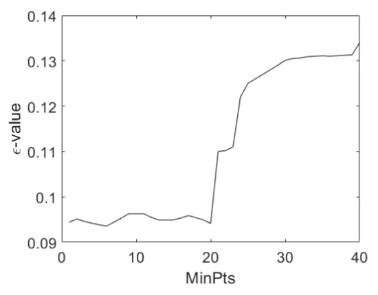
Figure 3.
as a function of for level noise.
s was related to the number of signals for an instant. Table 5 shows the effects of for three levels of noise. This table aimed to represent the effectiveness of the automatized and , with the initial state that is the Euclidean distance that exists in the OPTICS algorithm, and all the features (seventeen). From this table, the optimal value of was . This value of made it possible to detect the fault before the others.
Table 5.
Effect of on detection time, with Euclidian distance, 17 features, .
The selection of the distance measure affects the results of clustering algorithms. In this section, the advantages and disadvantages of every distance method used are shown in Table 6. The Euclidean distance used in the OPTICS algorithm in clustering, to calculate the distance between two vectors, was significantly difficult to iterate even an approximate of the precise values of data. Table 7 below shows the effect of distance implanted in the AOC-OPTICS method for three noise levels. The Manhattan distance could lead to the detection of the defect with global accuracy for the different signal to noise ratio equal to 96.7%, and then the second one was the Mahalanobis distance that detected at 88.2%, for the other distances the accuracy equaled 85.5%.
Table 6.
Advantages and disadvantages of different uses distance. and are features vectors.
Table 7.
Effect of distances, with , 17 features, .
4.3. Effect of Ranking Features
Usually ranking features is used in preprocessing data as a feature subdivision. The concept for use is to count the random instance, then calculate their nearest neighbors and set the vector of weighting features, which can distinguish the features from neighbors of various classes.
Two methods chi-square and relief were compared. Table 8 represents the result of the ranking features. The comparative study presents the effectiveness of the relief method that could detect the defect in the high accuracy from features number ten to the end. The chi-square start to recognize the highest efficiency with twelve features. From the results of Table 8 could conclude that the method of relief ranking features was the best with just ten features that was enough to obtain the highest accuracy.
Table 8.
Global accuracy. Effect of ranking features with Manhattan distance, , .
4.4. Results
In this section, the results were obtained for the following parameters: relief method, distance from Manhattan, and . A 3D visualization was chosen (three principal components). In fact, the 3D results gave a detection accuracy of 96.7% and the 2D results covered an accuracy of less than 93.7%. The results of the BPFO (ball pass frequency outer) simulation showed the fault detected from signal A11, for noise levels 0.1b (t), 0.3 b(t) and for 0.5b (t) (Figure 4, Figure 5 and Figure 6).
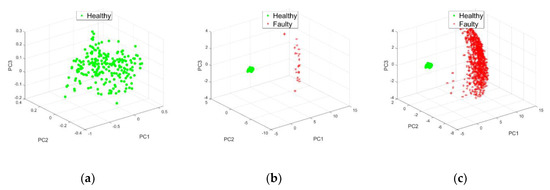
Figure 4.
Effect of amplitude 0.1b (t): (a) , (b) and (c) .
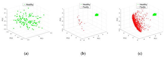
Figure 5.
Effect of amplitude 0.3b (t): (a) , (b) and (c) .
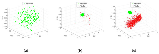
Figure 6.
Effect of amplitude 0.5b (t): (a) , (b) and (c) .
The follow-up starting after the end of the detection phase. monitors the growth of the fault with the varied amplitude of signals. The evolution of was studied for the three noise levels 0.1b (t), 0.3b (t) and 0.5b (t), Figure 7.
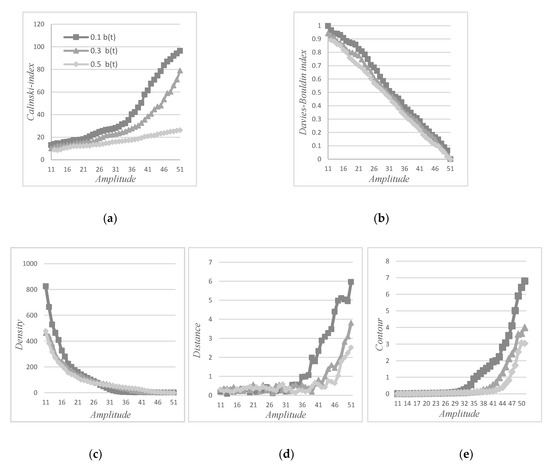
Figure 7.
(a) Calinski index, (b) Davies–Bouldin index, (c) density, (d) distance and (e) contour.
Figure 7a represents the Calinski index calculated between the two clusters. The curve values increased with increasing amplitude values. The Calinski index value for the 0.1b (t) was more significant and the curve was above the others. For a high noise level, the evolution was linear , while for the other two noise levels the evolution was exponential (.
Figure 7b represents the Davies–Bouldin index, the curve was the opposite of the Calinski-Harabasz index, which decreased with the increasing amplitude of signals. The results observed here showed a curve of 0.1b (t), which was above the other curves, and started near to one and ended near-zero. For the three noise levels, the regression was linear. The mathematical model was similar: respectively for 0.1b (t), 0.3b (t) and 0.5b (t).
Figure 7c represents the density of the defected cluster or the second class. The density decreases over the amplitude of signals until it became constantly equal to zero, contrary to the Davies–Bouldin index decrease, to attend near zero at the end of class. The comparison between the curves showed that the density of 0.1b (t), bigger than the other noise to signal ratios. The evolution was exponential with the mathematical model: , 0.1b (t), 0.3b (t) and 0.5b (t). The correlation was poor for a low noise level.
Figure 7d represents the distance between two clusters, the distance values growing with amplitude. However, the curvy curve had an increasing trajectory form for the three scenarios 0.1b (t), 0.3b (t) and 0.5b (t). Additionally, the distance parameter could observe the trajectory of 0.1b (t), was above the other curves at the end, but initially, the three curves were conjoined, then started to separate from an amplitude equal to . A linear model mathematic measurement could be done from , .
Figure 7e represents the contour of the second cluster, showing the increase of contour with the amplitude of signals. The comparison of the contour with the Calinski index shows, the Calinski index remained increasing with the number of amplitudes. However, the contour values were similar for noise levels at low amplitudes. The contour was relevant for a certain amplitude level, for low noise levels and for higher noise levels. The regression models starting from were .
In summary, the Calinski index differentiates noise levels for all amplitudes. However, the mathematical regression model was different. For low noise levels, a linear model was interesting, while for high noise levels, the exponential model was preferred. On the contrary, the Calinski index was little influenced by the noise level, thus the linear regression model was relevant and similar. That could show the importance of the Calinski index, which could separate the curves of different scenarios, the value started with zero and grew directly with the amplitude, while the contour parameter increased slowly with the amplitude. The parameters, density and distance, had values close to 0 either for low amplitudes or high amplitudes. The evolutions were only visible for ranges of amplitudes. According to these simulations the Calinski and Davies–Bouldin indexes were preferred.
This numerical investigation made it possible to fix the internal parameters OPTICS, (Equation (4)), ) and to optimize the methods involved in the AOC-OPTICS process (relief method, t-SNE and Manhattan distance).
5. Experimental Validation
5.1. Test Bench
The experimental bench consists of a crankcase connected with the electric motor of 10 KW maximum power through a shaft and two rolling bearings: healthy (6206 ball bearing) and degraded (N.206.E. G15 roller bearing), Figure 8. A hydraulic jack via steel cable was used to vary loads on the shaft (Figure 8a). The motor has rotational speed controlled by variable speed drive. The whole device was built to a concrete structure to isolate it from the low frequencies generated by the external environment. A piezoelectric sensor was placed radially on the bearing, considered as the best measuring point. The data were collected with a sampling frequency of 51,200 Hz. Eight defects on the outer ring of the roller bearing were created with an electro pen. The defects were measured using a paste mark "plastiform", Table 9. The resulting profile was characterized as roughness, with a Taylor-Hobson subtronic 3P profilometer (Figure 8b). For the nine states of the defect (one healthy and eight defect sizes), 10 randomly operating conditions were applied among 5 loads ranging from 100 to 220 daN, with a 30 daN step, and 5 rotation speed varies ranging from 1405 to 1560 rpm with a 50 rpm step. The number of combinations was 90 (). For each combination 8 signals were collected with 12,800 samples. The total database was made of 720 signals.
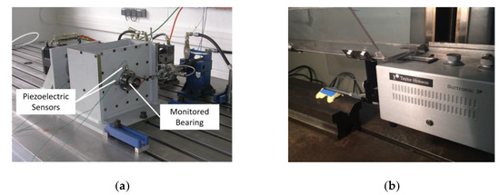
Figure 8.
(a) Test bench (b) profilometer with PlastiformTM paste.
Table 9.
Dimensions of the defects: width (W), arithmetic roughness (Ra) and total roughness (Rt).
AOC-OPTICS method was applied. The inputs were and . Thus, at each iteration , 8 new signals integrated the algorithm. Eighty signals initiated the monitoring process.
5.2. Results
After the initialization phase , the detection phase operated during the detection of a second class. This detection was made for the iteration . The inputs parameters were and . Results of AOC-OPTICS method are represented in Figure 9. The cluster number 2 appeared at iteration 11 and was confirmed by the following iterations. Despite the variation of loads and speed the accuracy was 100%. The results of our methodology could detect a tiny variation in the state of the bearing. All these results could demonstrate the robustness of the used methodology.
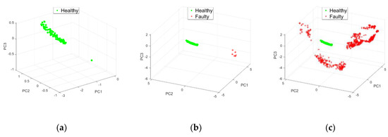
Figure 9.
Experimental validation (a) Iteration 10, (b) Iteration 11 and (c) Iteration 90.
5.3. Follow-Up
The follow-up starts at iteration 11 to iteration 90 for the 5 , Calinski and Davies–Bouldin index, density, contour and distance, Figure 10. The behavior of these variables was different and remained similar to the behaviors established during the simulation. The Calinski index increased with the size of defects. At iteration 65, the index had an exponential evolution in the mathematical form , Figure 10a. The Davies–Bouldin index decreased proportionally with the fault, Figure 10b. In this case, a linear regression was proposed. The density decreased with the increasing amplitude values to attend around zero from signal number sixty to ninety, the mathematical model was . The distance curve was increasing with the increasing of the amplitude values. The evolution was exponential However the monotony was not relevant. There was a lot of variability around the average trend, Figure 10d. The contour shows two trends, Figure 10e. The contour evolved proportionally for the first 60 iterations with a low slope, . From the 60th iteration onwards, the evolution remained linear but increased sharply, .
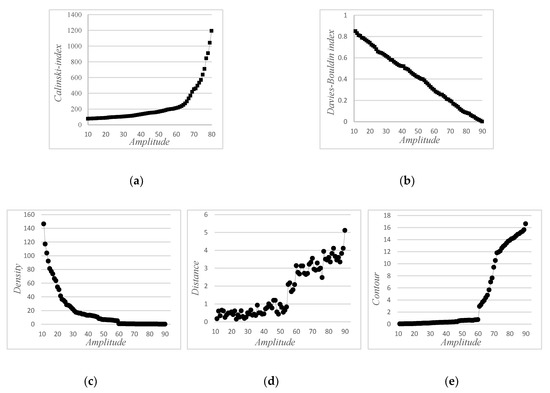
Figure 10.
Follow-up of the detected cluster: evolution of (a) Calinski index, (b) Davies–Bouldin index. (c) Density, (d) distance and (e) contour.
By comparing the evolution of these indicators, the Calinski index and the contour showed some singularities in the evolution at iteration 60 corresponding to defect 5. These parameters indicate the severity degradation stage in the rolling bearing. The Davies-Bouldin index was the index most correlated to the number of iteration (. In general, these indicators allowed us to make a prognosis on the evolution of these parameters with the iterations.
6. Conclusions
This paper proposed an automatic online methodology for monitoring ball bearings by optimizing the internal parameters of the OPTICS method and the dimension reduction step. The dynamic monitoring AOC-OPTICS was divided into three phases: the initialization, the detection and following the defect. The methodology was confronted with a simulated fault evolution and then with experimental data. The detection reached an accuracy of 100%. The follow-up was assured by geometrical values whose trend followed linear or exponential mathematical models with correlation coefficients up to 0.994. This methodology brings many improvements: (I) This automated methodology used the best parameters for the detection and following the defects with high accuracy. (II) The variation of speed and load cannot lead to discovering the fault in the rolling bearing. Only the amplitude leads to detecting the faulty state. (III) The relief method is efficient compared to chi-square, which is used to delete unnecessary features, which can make the iteration to be calculated speedily. (IV) The characteristics parameters related to the defect facilitate monitoring of the evolution with the times. (V) The density and Calinski and Davies–Bouldin index represent efficacy more than the other parameters, for monitoring the defect growth trajectory. The major perspective is to add the diagnostic part in the methodology to increase the prognosis. This part must be based on previous knowledge provided by a digital twin or an expert.
Author Contributions
H.H. performed the experiments, conceived the algorithm and analyzed the data. X.C. and L.R. planned the experiments and supervised the research work. H.H. and X.C. wrote the paper and L.R. revised the entire paper. All authors have read and agreed to the published version of the manuscript.
Funding
This research received no external funding.
Conflicts of Interest
The authors declare no conflict of interest.
References
- Xenakis, A.; Karageorgos, A.; Efthimios, L.; Chis, A.E.; González-Vélez, H. Towards Distributed IoT/Cloud based Fault Detection and Maintenance in Industrial Automation. Procedia Comput. Sci. 2019, 151, 683–690. [Google Scholar] [CrossRef]
- Yan, J.; Meng, Y.; Lu, L.; Li, L. Industrial Big Data in an Industry 4.0 Environment: Challenges, Schemes, and Applications for Predictive Maintenance. IEEE Access 2017, 5, 23484–23491. [Google Scholar] [CrossRef]
- Short, M.; Twiddle, J. An Industrial Digitalization Platform for Condition Monitoring and Predictive Maintenance of Pumping Equipment. Sensors (Switzerland) 2019, 19, 3781. [Google Scholar] [CrossRef] [PubMed]
- Harris, T.A.; Kotzalas, M.N. Rolling Bearing Analysis, 5th ed.; Taylor & Francis: Boca Raton, FL, USA, 2006. [Google Scholar]
- Sri, J.; Senanayaka, L.; Kandukuri, S.T.; Van Khang, H.; Robbersmyr, K.G. Early Detection and Classification of Bearing Faults Using Support Vector Machine Algorithm. In Proceedings of the 2017 IEEE Workshop on Electrical Machines Design, Control and Diagnosis (WEMDCD), Nottingham, UK, 20–21 April 2017. [Google Scholar] [CrossRef]
- Li, Z.; Zhu, J.; Shen, X.; Zhang, C.; Guo, J. Fault diagnosis of motor bearing based on the Bayesian network. Procedia Eng. 2011, 16, 18–26. [Google Scholar] [CrossRef][Green Version]
- Tian, J.; Azarian, M.H.; Pecht, M. Rolling Element Bearing Fault Detection Using Density-Based Clustering. In Proceedings of the 2014 International Conference on Prognostics and Health Management, Cheney, WA, USA, 22–25 June 2014. [Google Scholar] [CrossRef]
- El-thalji, I.; Jantunen, E. A Summary of Fault Modelling and Predictive Health Monitoring of Rolling Element Bearings. Mech. Syst. Signal Process. 2015, 60–61, 252–272. [Google Scholar] [CrossRef]
- Cerrada, M.; Sánchez, R.V.; Li, C.; Pacheco, F.; Cabrera, D.; Valente de Oliveira, J.; Vásquez, R.E. A Review on Data-Driven Fault Severity Assessment in Rolling Bearings. Mech. Syst. Signal Process. 2018, 99, 169–196. [Google Scholar] [CrossRef]
- Brijesh, S.; Dushyanth, N.D.; Soumendu, J.; Sarvajith, M. A Novel Approach for Bearing Fault Detection and Classification Using Acoustic Emission Technique. In Proceedings of the First International Conference on Advances in Computer, Electronics and Electrical Engineering—CEEE 2012, Mumbai, India, 25–27 March 2012. [Google Scholar]
- Stein, B.; Busch, M. Density-Based Cluster Algorithms in Low-Dimensional and High-Dimensional Applications. In Proceedings of the Second International Workshop on Text-Based Information Retrieval, Koblenz, Germany, 11 September 2005; pp. 45–55. [Google Scholar]
- Wei, Z.; Wang, Y.; He, S.; Bao, J. A Novel Intelligent Method for Bearing Fault Diagnosis Based on Affinity Propagation Clustering and Adaptive Feature Selection. Knowledge-Based Syst. 2017, 116, 1–12. [Google Scholar] [CrossRef]
- Ankerst, M.; Breunig, M.M.; Kriegel, H.P.; Sander, J. OPTICS: Ordering Points to Identify the Clustering Structure. ACM SIGMOD Record 1999, 28, 49–60. [Google Scholar] [CrossRef]
- Shah, G.H.; Bhensdadia, C.K.; Ganatra, A.P. An Empirical Evaluation of Density-Based Clustering Techniques. Int. J. Soft Comput. Eng. IJSCE 2012, 1, 216–223. [Google Scholar]
- Benmahdi, D.; Rasolofondraibe, L.; Chiementin, X.; Murer, S.; Felkaoui, A. RT-OPTICS: Real-Time Classification Based on OPTICS Method to Monitor Bearings Faults. J. Intell. Manuf. 2019, 30, 2157–2170. [Google Scholar] [CrossRef]
- Urbanowicz, R.J.; Meeker, M.; Cava, W.L.; Olson, R.S.; Moore, J.H. Relief-Based Feature Selection: Introduction and Review. J. Biomed. Inform. 2018, 85, 189–203. [Google Scholar] [CrossRef] [PubMed]
- Vakharia, V.; Gupta, V.K.; Kankar, P.K. Bearing Fault Diagnosis Using Feature Ranking Methods and Fault Identification Algorithms. Procedia Eng. 2016, 144, 343–350. [Google Scholar] [CrossRef][Green Version]
- Xie, Y. A Fault Diagnosis Approach Using SVM with Data Dimension Reduction by PCA and LDA Method. In Proceedings of the 2015 Chinese Automation Congress (CAC), Wuhan, China, 27–29 November 2015. [Google Scholar] [CrossRef]
- Deng, F.; Ren, B. Fault Diagnosis of Rolling Bearing Using the Hermitian Wavelet Analysis, KPCA and SVM. In Proceedings of the 2017 International Conference on Sensing, Diagnostics, Prognostics, and Control (SDPC), Shanghai, China, 16–18 August 2017. [Google Scholar] [CrossRef]
- Tu, D.; Zheng, J.; Jiang, Z.; Pan, H. Multiscale Distribution Entropy and T-Distributed Stochastic Neighbor Embedding-Based Fault Diagnosis of Rolling Bearings. Entropy 2018, 20, 360. [Google Scholar] [CrossRef]
- Ozkok, F.O.; Celik, M. A New Approach to Determine Eps Parameter of DBSCAN Algorithm. Intell. Syst. Appl. Eng. 2017, 5, 247–251. [Google Scholar] [CrossRef][Green Version]
- Loohach, R.; Garg, K. Effect of Distance Functions on Simple K-Means Clustering Algorithm. Int. J. Comput. Appl. 2012, 49, 7–9. [Google Scholar] [CrossRef]
- Shukla, S. Analysis of Statistical Features for Fault Detection. In Proceedings of the IEEE International Conference on Computational Intelligence and Computing Research (ICCIC), Madurai, India, 10–12 December 2015. [Google Scholar]
- Cai, J.; Xiao, Y. Time-Frequency Analysis Method of Bearing Fault Diagnosis Based on the Generalized S Transformation. J. Vibroeng. 2017, 19, 4221–4230. [Google Scholar] [CrossRef]
- Qian, Y.; Yan, R.; Gao, R.X. A Multi-Time Scale Approach to Remaining Useful Life Prediction in Rolling Bearing. Mech. Syst. Signal Process. 2017, 83, 549–567. [Google Scholar] [CrossRef]
- Vakharia, V.; Gupta, V.K.; Kankar, P.K. A comparison of feature ranking techniques for fault diagnosis of ball bearing. Soft Comput. 2016, 20, 1601–1619. [Google Scholar] [CrossRef]
- Chiementin, X. Localization and quantification of vibratory sources for a predictive maintenance in order to increase the diagnosis and the follow-up of the damage of the rotating mechanical components: Application to rolling bearings. Ph.D. Thesis, University of Reims Champagne-Ardenne, Reims, France, October 2007. [Google Scholar]
- Jain, A.K.; Murty, M.N.; Flynn, P.J. Data clustering: A review. ACM Comput. Surv. 1999, 31, 264–323. [Google Scholar] [CrossRef]
- Pandit, S.; Gupta, S. A Comparative Study on Distance Measuring Approaches for Clustering. Int. J. Res. Comput. Sci. 2011, 2, 29–31. [Google Scholar]
- Durak, B. A Classification Algorithm Using Mahalanobis Distances Clustering of Data with Applications on Biomedical Data Set. Master’s Thesis, Middle East Technical University, Bahadır, Turkey, January 2011. [Google Scholar]
- Krishnan, S.; Kerkhoff, H.G. Exploiting Multiple Mahalanobis Distance Metrics to Screen Outliers from Analog Product Manufacturing Test Responses. IEEE Des. Test 2013, 30, 18–24. [Google Scholar] [CrossRef]
- Egan, W.J.; Morgan, S.L. Outlier Detection in Multivariate Analytical Chemical Data. Anal. Chem. 1998, 70, 2372–2379. [Google Scholar] [CrossRef] [PubMed]
- Taylor, P.; Hadi, A.S.; Simonoff, J.S.; Hadi, A.S.; Simonoff, J.S. Procedures for the Identification of Multiple Outliers in Linear Models Procedures for the Identification of Multiple Outliers in Linear Models. J. Am. Stat. Assoc. 2012, 88, 37–41. [Google Scholar] [CrossRef]
- Soler, J.; Tencé, F.; Gaubert, L.; Buche, C. Data Clustering and Similarity. In Proceedings of the Twenty-Sixth International Florida Artificial Intelligence Research Society Conference, Pete Beach, FL, USA, 22–24 May 2013; pp. 492–495. [Google Scholar]
- Xu, R.; Member, S.; Ii, D.W. Survey of Clustering Algorithms. IEEE Trans. Neural Netw. 2005, 16, 645–678. [Google Scholar] [CrossRef] [PubMed]
- Potolea, R.; Cacoveanu, S.; Lemnaru, C. Meta-learning Framework for Prediction Strategy Evaluation. In Proceedings of the International Conference on Enterprise Information Systems, Funchal-Madeira, Portugal, 8–12 June 2010; pp. 280–295. [Google Scholar]
- Bellet, A.; Habrard, A.; Sebban, M. A Survey on Metric Learning for Feature Vectors and Structured Data; Technical Report; Cornell University: Ithaca, NY, USA, 2013. [Google Scholar]
© 2020 by the authors. Licensee MDPI, Basel, Switzerland. This article is an open access article distributed under the terms and conditions of the Creative Commons Attribution (CC BY) license (http://creativecommons.org/licenses/by/4.0/).