Integrating Support Vector Regression with Genetic Algorithm for Hydrate Formation Condition Prediction

Abstract

To predict the natural gas hydrate formation conditions quickly and accurately, a novel hybrid genetic algorithm–support vector machine (GA-SVM) model was developed. The input variables of the model are the relative molecular weight of the natural gas (M) and the hydrate formation pressure (P). The output variable is the hydrate formation temperature (T). Among 10 gas samples, 457 of 688 data points were used for training to identify the optimal support vector machine (SVM) model structure. The remaining 231 data points were used to evaluate the generalisation capability of the best trained SVM model. Comparisons with nine other models and analysis of the outlier detection revealed that the GA-SVM model had the smallest average absolute relative deviation (0.04%). Additionally, the proposed GA-SVM model had the smallest amount of outlier data and the best stability in predicting the gas hydrate formation conditions in the gas relative molecular weight range of 15.64–28.97 g/mol and the natural gas pressure range of 367.65–33,948.90 kPa. The present study provides a new approach for accurately predicting the gas hydrate formation conditions.

1. Introduction

Natural gas hydrate is a dry ice-like crystalline inclusion compound formed by combining small gas molecules (e.g., light hydrocarbons, CO₂, H₂S, or N₂) and water molecules in natural gas under certain pressure and temperature conditions. In industrial production, hydrates are widely used for gas storage and refrigeration. In the process of oil and gas field development, hydrate formation leads to engineering accidents. The formation of hydrates can easily block wellbores and reservoirs near gas wells, which results in a reduction or even shutdown of the gas-well production. Additionally, the formation of hydrates can block measurement instruments, surface separation equipment, and gas pipelines, which causes a pipeline rupture. It may even cause explosions. Therefore, it is important to accurately predict the formation conditions of natural gas hydrates.

Currently, the main determination methods for natural gas hydrate formation are experimental methods [1,2,3], formula methods [4], thermodynamic models [5,6], and intelligent models [7,8]. Experiments to determine the conditions for forming natural gas hydrates yield the most accurate results, but the experimental methods are time-consuming, laborious, and expensive. Formula methods are widely used because they are facile and involve easy programming. The widely used correlation formulas include those proposed by Ponomape [9], Bohadori-Vuthalur [10], Chayyem [11], and Amin [12]. Chayyem established an association formula based on a Katz gravity map for 545 data points, which exhibited the highest prediction accuracy among the previously mentioned formulas [13]. However, the formula method has a limited range, beyond which the calculation error is relatively large. Thermodynamic models are usually derived from the VdwP model proposed by Van der Waals and Platteeuw in 1959. The thermal equilibrium model equation is based on the thermodynamic theory. A numerical method is used to perform the calculations. Currently, the main models include those proposed by Parrish and Pransnitz [14], Chen and Guo [15], and Klauda and Sandler [16]. However, assumptions are made in establishing the models, and the errors of the models in practical applications are relatively large. Moreover, the models are complex and difficult to generalise [17,18]. Research on predicting the conditions for natural gas hydrate formation using intelligent algorithms (such as the backpropagation (BP) neural network and support vector machine (SVM)) has developed rapidly in recent years and yielded good results. Wu Xiaoqiang, Han Bing [19] established a prediction model for the natural gas hydrate formation conditions under a high-H₂S and high-CO₂ environment based on an SVM by introducing a factor reflecting the contribution of acid gas (H₂S+CO₂) to the formation of CH₄. To solve the problems of the large-scale secondary planning and low calculation speed of the SVM, Mesbah et al. [20] used the least-squares SVM method to predict the desulfurisation and temperature of acid gas-containing hydrates. In the same year, Mohammad Akbari as well as Afshin et al. [21] used the temperature, pressure, and natural-gas composition as input variables and combined radial basis function (RBF) neural networks with genetic algorithms (GAs) to predict conditions for natural gas hydrate formation at low temperatures. However, in this method, the number of nodes in the hidden layer and the weight threshold must be determined, and it is difficult to identify the optimal network structure parameters [22,23,24].

In this study, a GA was used to optimise the process parameters of an SVM, and a new hybrid model (GA-SVM) was developed for predicting the conditions of natural gas hydrate formation. The model takes the relative molecular weight of the natural gas and the hydrate formation pressure as input variables and outputs the hydrate formation temperature. Through example calculations, the GA-SVM model was compared with nine commonly used models. Using the leverage method, outlier detection was performed for 688 data points. This study provides a comprehensive method for the accurate prediction of the gas hydrate formation conditions.

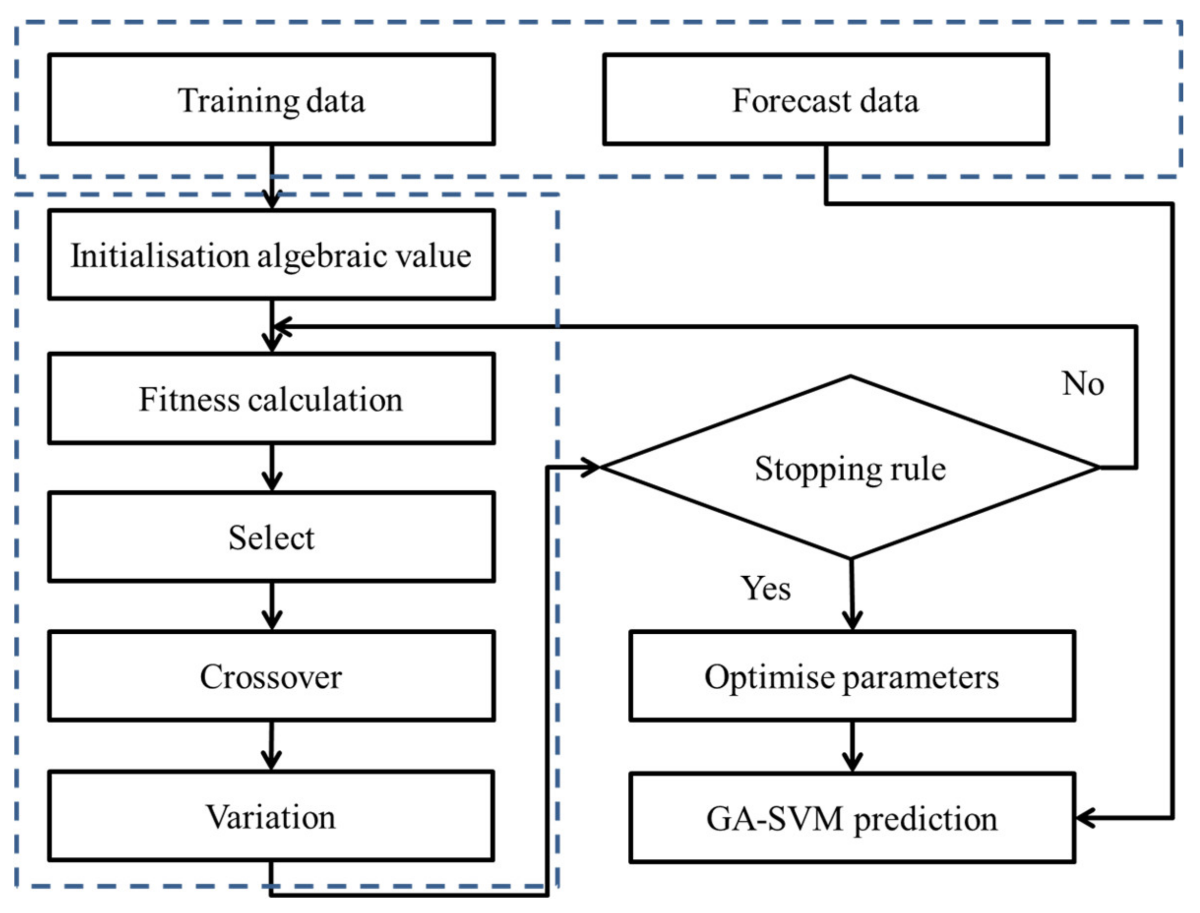
2. Theoretical Basis

Support vector machines (SVM) are a kind of binary classification model. Its purpose is to find a hyperplane to segment the samples. The principle of segmentation is to maximise the interval, which is eventually transformed into a convex quadratic programming problem to solve [25]. Rather than relying on the general rule of empirical risk minimisation, it employs the structural risk-minimisation function, which significantly improves its efficiency for solving the multivariate nonlinear regression problem. Advanced optimisation algorithms (e.g., genetic algorithm, particle swarm algorithm, grey wolf algorithm) are used to avoid the problems related to local optima and non-convergence that easily occur in other machine-learning algorithms, such as the classic back propagation neural network, and overcome the difficulties of other machine-learning algorithms, e.g., a small amount of data samples, rough data, and large data volatility [26].

The basic idea of the SVM nonlinear regression model is to transform a nonlinear regression problem in a low-dimensional space into a linear regression problem in a high-dimensional feature space through nonlinear mapping [27]. In this way, the linear regression can be better fitted through a reasonable feature surface in high-dimensional space. Accordingly, the algorithm of the SVM dual optimisation problem is as follows.

Given a dataset {(xi, yi), i = 1,2,…, N}, its basic regression function is

$$f(x)=〈w,x〉+b.$$

(1)

The structural risk function used in SVM regression is

$$R(f)=\frac{1}{N}{\displaystyle \sum _{i=1}^{N}L(f(x_i)-y_i)}+\frac{1}{2}{‖w‖}^2.$$

(2)

The loss function in Equation (2) is

$$L(f(x)-y)=\left\{\begin{array}{l}‖L(f(x)-y)‖-\epsilon ,\hspace{1em}\left|f(x)-y\right|\ge \epsilon \\ 0\hspace{1em}\hspace{1em}\hspace{1em}\hspace{1em}\hspace{1em}\hspace{1em}\hspace{1em}\left|f(x)-y\right|<\epsilon \end{array}\right..$$

(3)

By substituting Equation (3) into Equation (2) and introducing the relaxation variables ξ and ξ*, the objective function can be obtained:

$$\mathrm{minimise} \frac{1}{2}{‖w‖}^2+C{\displaystyle \sum _{\mathrm{i}=1}^N\left(\xi +{\xi }^{*}\right)}$$

(4)

$$\mathrm{s}.\mathrm{t}. \left\{\begin{array}{l}{\mathrm{y}}_{\mathrm{i}}-〈w,x_i〉+b\le \epsilon +{\xi }_i\\ 〈w,x_i〉+b-{\mathrm{y}}_{\mathrm{i}}\le \epsilon +{\xi }_i^{\ast }\\ {\xi }_i,{\xi }_i^{\ast }\ge 0\\ i=1,2,\dots ,N\end{array}\right..$$

(5)

Equation (4) introduces the Lagrange function. Dual processing is performed, which yields the following.

$$\mathrm{maximise} -\frac{1}{2}{\displaystyle \sum _{i,j=1}^N\left({\alpha }_i-{\alpha }_i^{*}\right)}\left({\alpha }_j-{\alpha }_j^{*}\right)\left(x_i,x_j\right)-\epsilon {\displaystyle \sum _{\mathrm{i}=1}^N\left({\alpha }_i+{\alpha }_i^{*}\right)}+{\displaystyle \sum _{i=1}^N{y}_i\left({\alpha }_i-{\alpha }_i^{*}\right)}$$

(6)

$$s.t.\left\{\begin{array}{l}{\displaystyle \sum _{i=1}^N\left({\alpha }_i-{\alpha }_i^{\ast }\right)=0}\\ 0\le {\alpha }_i\le C\\ 0\le {\alpha }_i^{\ast }\le C\\ i, \mathrm{j}=1,2,\dots ,N\end{array}\right..$$

(7)

Using Equations (6) and (7), the SVM regression model can be obtained.

$$f(x)=\left({\alpha }_{\mathrm{i}}-{\alpha }_{\mathrm{i}}^{\ast }\right)〈x_i,x〉+b$$

(8)

For the inner-product problem, There are four types of common kernel functions: linear kernel function, polynomial kernel function, radial basis function (RBF) kernel function and sigmoid kernel function. Among them, RBF kernel function has better performance and more applications. Therefore, in this paper, the internal product problem is replaced by RBF function, whose expression is as follows:

$$K\left(x_i,x_j\right)=\exp \left(-\gamma ‖x_i,x_j‖\right), \left(\gamma >0\right)$$

(9)

Eventually, the SVM regression model becomes the following.

$$f(x)=\left({\alpha }_{\mathrm{i}}-{\alpha }_{\mathrm{i}}^{\ast }\right)K\left(x_i,x\right)+b$$

(10)

In Equations (1)–(10),

ε represents the loss factor,

ξ and ξ* represent the relaxation variables,

C represents the penalty factor,

α_i and α_i^* represent the Lagrange multiplier pairs for each sample, and

γ represents the width parameter of the kernel function.

The GA is an advanced parameter-optimisation algorithm. The basic idea is to simulate the evolutionary law of biological competition, i.e., survival of the fittest, in the biological world [28,29]. The specific steps are as follows.

(1)

Random chromosome coding of individuals in the initial population using the binary principle to form a genotype string that mimics the chromosome of a biological gene, which is an individual in the biological population.

(2)

On the basis of step 1), the N initial genotype character strings are randomly generated to form an initial population containing N individuals.

(3)

The fitness function is defined, and the superiority and inferiority of the individuals in the population are evaluated (i.e., the solution of optimised parameters) by calculating the fitness values of the individuals.

(4)

Individuals are selected with a certain probability based on the fitness value. a smaller fitness value corresponds to a higher probability of being selected for the next-generation population.

(5)

On the basis of step (4), the individuals of the population are optimised through crossover and mutation with a certain probability to obtain individuals with better adaptability.

By using the Library for Support Vector Machines (LIBSVM) and genetic algorithm (GA) toolboxes in MATLAB (The toolbox is a set of simple and efficient software package for pattern recognition and nonlinear regression of support vector machine developed by Professor Lin Zhiren of Taiwan University) to perform extended programming, a GA-SVM hybrid model was developed. The specific process of the GA-SVM model training and prediction is shown in Figure 1.

3. Model Building

3.1. Dataset and Variable Selection

In the development of the GA-SVM model, the dataset diversity, variable selection, and parameter optimisation were mainly considered. To this end, 10 representative natural-gas samples were selected, and 688 gas samples in pure water hydrate formation conditions were used as experimental data points [30,31]. Some of the data is based on our experiments, and it is not easy to make public because of confidentiality. The dataset was randomly divided into two groups, i.e., 457 model training data and 231 model prediction data (ratio of 2:1). In the selection of the variables, considering the simplicity of the input variables of the GA-SVM model, the gas-sample composition was not selected as an input variable. Each gas sample was considered as a whole, and the relative molecular weight of the natural gas was used as an input variable. The input variables of the model were the relative molecular weight of the natural gas and the hydrate formation pressure, and the output variable of the model was the hydrate formation temperature. The variable ranges are presented in

Table 1. Variable ranges of the genetic algorithm–support vector machine (GA-SVM) model.

Variable	Relative Molecular Weight of Gas Sample (g/mol)	Pressure (KPa)	Temperature (K)
Range	15.64–28.97	367.65–33,948.90	273.20–298.84

.

As indicated by Table 1, the experimental data had a large step difference. To eliminate the effect of the data step on the model results, the ‘mapminmax’ function in MATLAB was used to normalise and de-normalise the data. The ‘mapminmax’ function is shown below.

$$\begin{array}{c}\overline{x}=2\frac{x-x_{\min }}{x_{\max }-x_{\min }}-1\end{array}(\overline{x}\in [-1,1])$$

(11)

where x represents the variable, $\stackrel{-}{x}$ represents the normalised variable value, x_max represents the maximum value of the variable, and x_min represents the minimum value of the variable.

3.2. Model Parameter Optimisation

According to the GA algorithm parameter optimisation process in flowchart 1, combined with the ‘trial calculation-control error’ method, there are three main parameters to be optimised: the penalty factor C, the width parameter γ of the kernel function, and the loss factor ε. In the process of parameter optimization, the value of penalty factor C has the greatest influence on the accuracy of the ε-SVM regression model. If the C value is too large, the fitting accuracy of training samples is very high, but the generalization ability of the ε-SVM regression model is very poor, there is a phenomenon of over learning. Similarly, if the C value is too small, the optimization process takes a long time, the search is not complete, the fitting effect of training samples is very poor, and the generalization ability of ε-SVM regression model is very low. Therefore, there is a serious phenomenon of under learning. Therefore, on the premise of not affecting the prediction accuracy, the C value should be as small as possible to ensure that the SVM regression model has good generalization ability and prediction accuracy. After several optimisation calculations, the optimal GA-SVM model parameters were determined, as shown in

Table 2. Optimal parameters of the GA-SVM model for gas hydrate formation.

Parameter Type	Optimise Parameters	Parameter Value (Range)
Variable value	Input data form	[−1,1]
genetic algorithm (GA) parameters	Evolutionary algebra	200
	Population size	20
	Selection probability	0.9
	Cross probability	0.7
	Mutation probability	0.035
support vector machine (SVM) parameters	Best C	854.8931
	Best ε	0.003592
	Best γ	9.1190

.

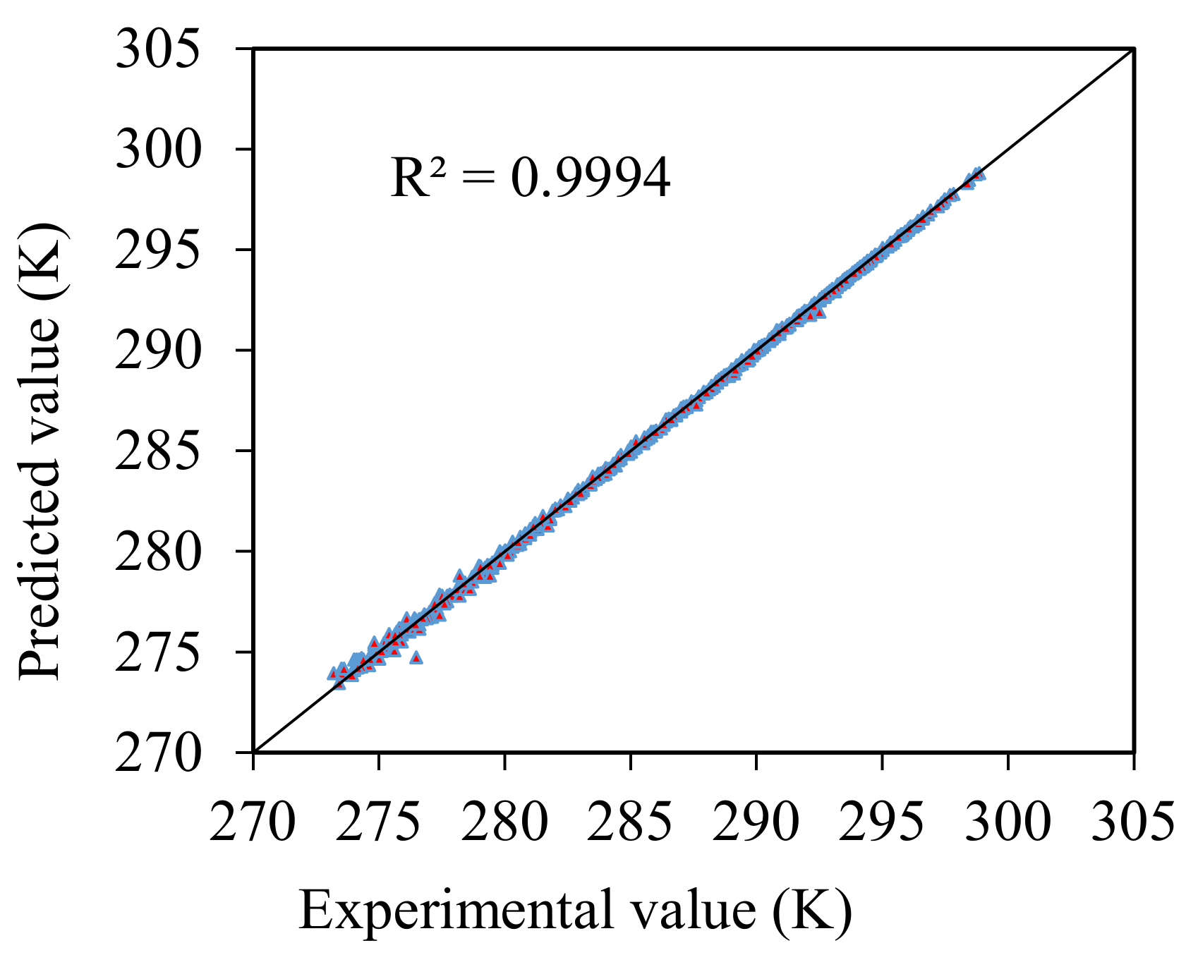
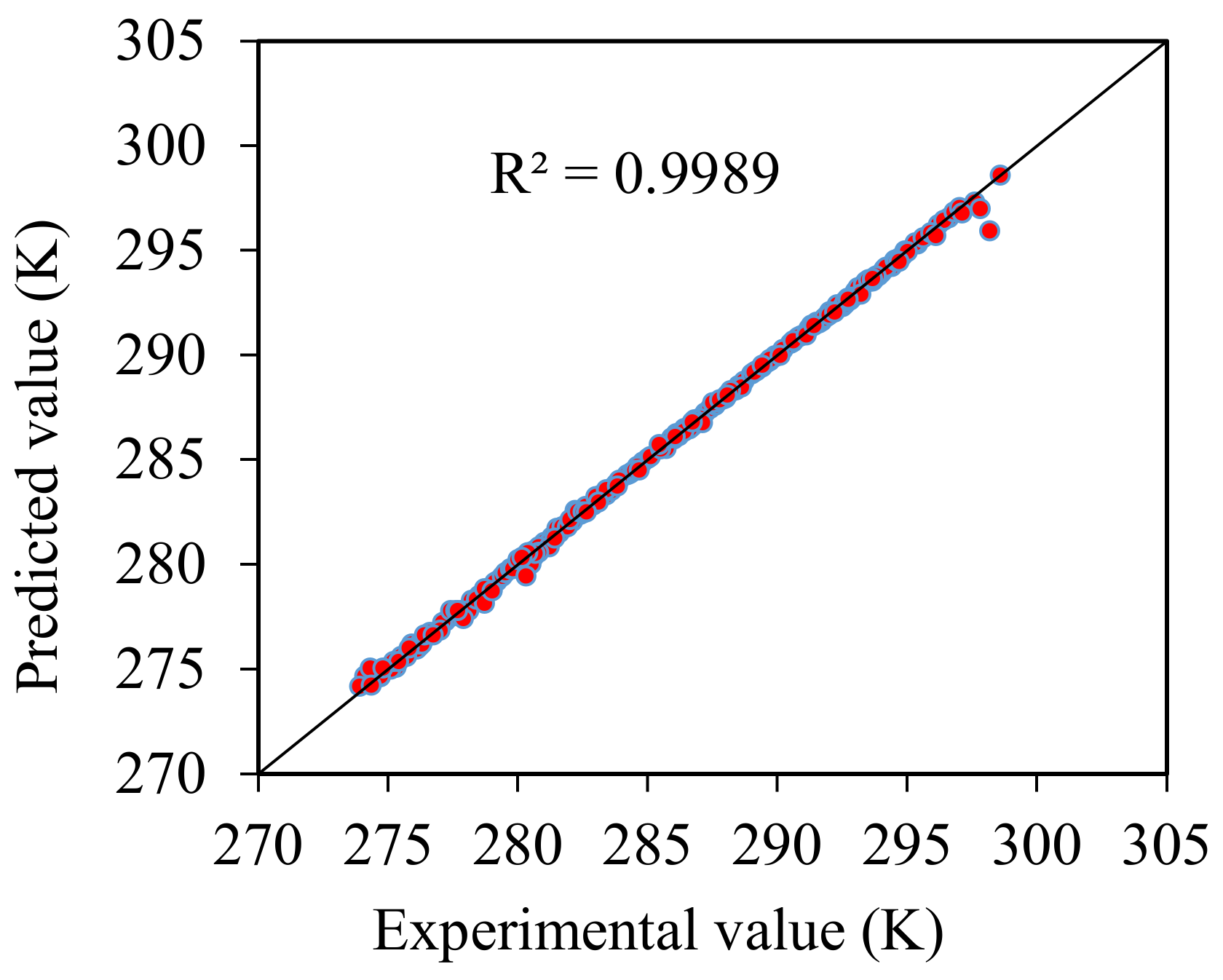
4. Analysis of Results

The results of the GA-SVM model training and prediction are presented in Figure 2 and Figure 3, respectively.

As shown in Figure 2 and Figure 3, the GA-SVM model exhibited good training and prediction results. The predicted and experimental values are evenly distributed around the 45° line, and the correlation coefficient (R²) is greater than 0.99. Thus, the model has good calculation accuracy and generalisation ability for predicting the natural gas hydrate formation conditions.

The mean absolute relative deviation (AARD) is defined as follows.

$$AARD=\frac{1}{n}{\displaystyle \sum _{i=1}^n\left|\frac{y_i^{\exp }-y_i^{pre}}{y_i^{\exp }}\right|}\times 100\%,$$

(12)

where $y_i^{exp}$ and $y_i^{exp}$ represent the experimental value of the i^th data point and the predicted value of the SVM model, respectively, and n represents the total number of data points.

To further evaluate the GA-SVM model, according to the calculation results of all the data points (688), the GA-SVM model was compared with the Ghayyem [11], Ann2015 [32], Zahedi (3), Zahedi (4) [33], Towler [22], Kobayashi [34], Hammerschmidt [35], Motiee [36], and Berge models [37]. The AARD results are shown in Figure 4.

As shown in Figure 4, among the 10 models for calculating the gas hydrate formation conditions, the GA-SVM model had the highest prediction accuracy, and the AARD was only 0.04%. For the Ghayyem, Ann2015, Zahedi (3), Zahedi (4), and Towler models, the AARDs were 0.14%, 0.46%, 0.56%, 0.56%, and 0.0.83%, respectively, and the calculation accuracy was relatively high. For the Berg model, the AARD was as high as 2.36%, and the calculation accuracy was poor.

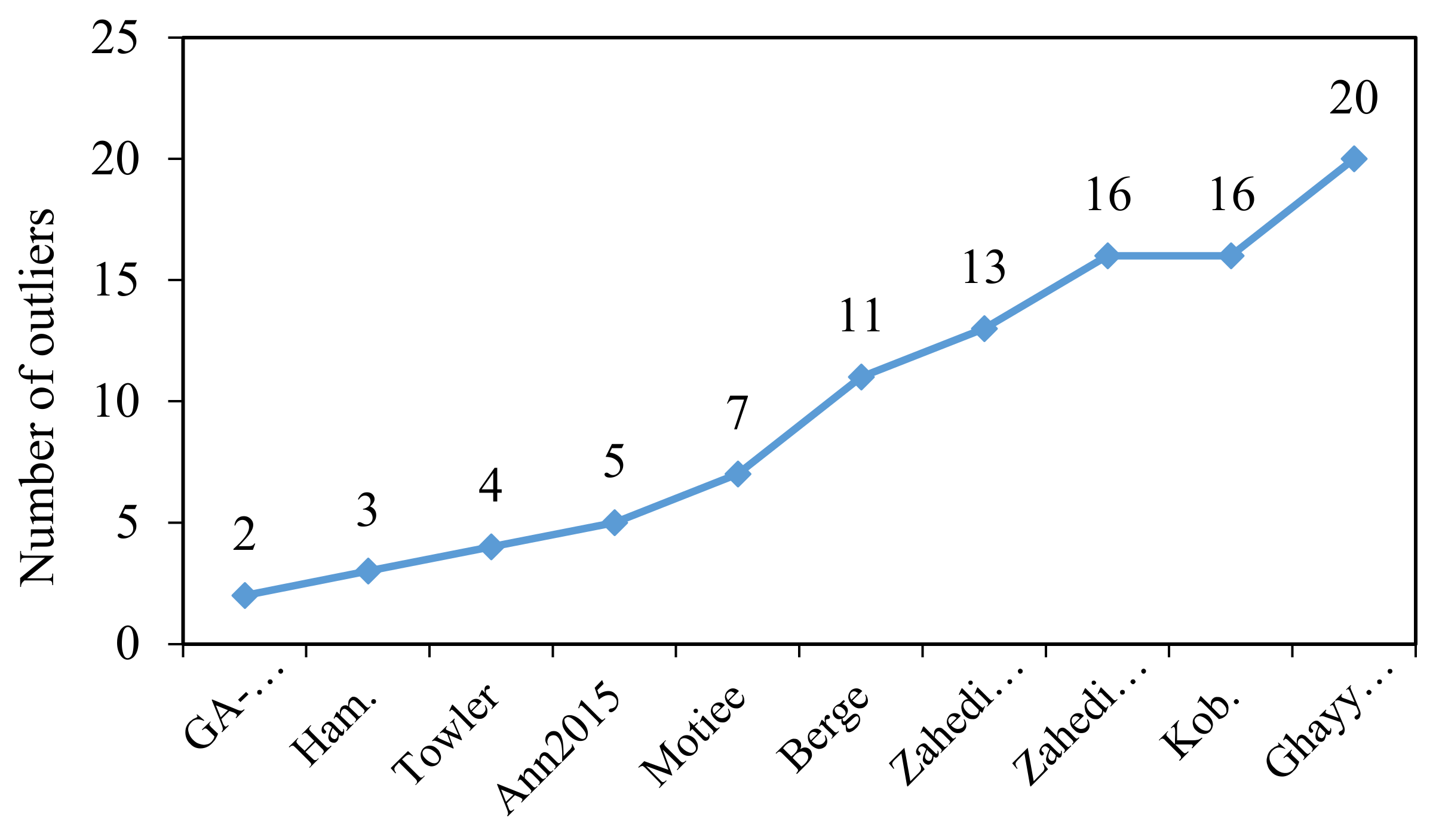
5. Outlier Detection

Artificial-intelligence algorithms have seen rapid development in recent years. Mohammadi et al. [38] proposed a new technology that can efficiently detect the abnormal points of a model via the Rousseeuw outlier detection theory–Williams plate detection method. The basic idea is to use the H value of the hat matrix and the standardised deviation between the model experimental data and the calculated data with the H value as the abscissa and the normalised deviation as the ordinate. The calculations of the model are performed on the premise of setting the leverage value. Consequently, abnormal points are detected. The specific steps of its algorithm are as follows.

First, the hat matrix is defined below.

$$H=X({X^{T}X)}^{-1}{X}^T,$$

(13)

where X represents an n × 2 matrix, which is composed of an SVM model predictor column vector and an input variable number vector. The leverage of the H value is set as the following.

H^*=3(m+1)/n,

(14)

where m represents the number of input variables, and n represents the number of experimental data points. The effective range of the H value is 0 ≤ H ≤ H*.

The SVM model standardised residual (SR) is defined as the following.

$$SR=\frac{y_i^{\exp }-y_i^{pre}}{\sqrt{\frac{1}{n-m-1}{\displaystyle {\displaystyle \sum }_{i=1}^n}{\left(y_i^{\exp }-y_i^{pre}\right)}^2\left(1-H_{ii}\right)}},$$

(15)

where H_ii represents the diagonal element of the hat matrix for the i^th data point. For model standardization residual (SR), the effective range is generally selected as −3 ≤ SR ≤ 3.

The H value and SR for the 10 models were calculated via the foregoing method. A Williams plot is constructed with the H value as the abscissa and the standardization residual (SR) as the ordinate, as shown in Figure 5. The number of abnormal points in each model is shown in Figure 6.

As shown in Figure 5 and Figure 6, the GA-SVM model had the smallest number of abnormal points in the 688 data (only two), which indicates that this model had good stability for predicting the natural gas hydrate formation conditions. The Ghayyem model had 20 anomalous points. A larger number of anomalous points indicates greater instability of the model in calculating the natural gas hydrate formation conditions.

6. Conclusions

By combining a GA, the outlier detection method, and an SVM, a new model for predicting the conditions of natural gas hydrate formation was developed. Comparisons with nine other models and analysis of the outlier detection revealed that the GA-SVM model had the smallest average absolute relative deviation (0.04%) in the gas relative molecular weight range of 15.64–28.97 g/mol and the natural gas pressure range of 367.65–33,948.90 kPa. Lastly, based on the leverage method, the abnormal point detection of all the data of all models was carried out. It was found that, in the 688 data points, the number of abnormal points of the GA-SVM model data was the lowest. There were only two abnormal points, which further illustrates that the GA-SVM model’s calculation of hydrate formation conditions has good stability.

References

1. Naeiji, P.; Varaminian, F. Experimental study and kinetics modeling of gas hydrate formation of methane-ethane mixture. J. Non-Equilib. Thermodyn. 2013, 38, 273–286. [Google Scholar]
2. Kar, S.; Kakati, H.; Mandal, A.; Laik, S. Experimental and modeling study of kinetics for methane hydrate formation in a crude oil-in-water emulsion. Pet. Sci. 2016, 13, 489–495. [Google Scholar]
3. Wu, W.; Guan, J.; Liang, D. The experimental research for structure H hydrate formation. J. Eng. Thermophys. 2018, 44–48. [Google Scholar]
4. Mottahedin, M.; Varaminian, F.; Mafakheri, K. Modeling of methane and ethane hydrate formation kinetics based on non-equilibrium thermodynamics. J. Non-Equilib. Thermodyn. 2011, 36, 3–22. [Google Scholar]
5. Obanijesu, E.O.; Gubner, R.; Barifcani, A.; Pareek, V.; Tade, M.O. The influence of corrosion inhibitors on hydrate formation temperature along the subsea natural gas pipelines. J. Pet. Sci. Eng. 2014, 120, 239–252. [Google Scholar]
6. Ma, S.; Huang, J.; Zhang, F. Prediction and prevention of hydrate forming in deep water gas well test. J. Xi’an Shiyou Univ. 2017, 6, 93–98. [Google Scholar]
7. Ghavipour, M.; Ghavipour, M.; Chitsazan, M.; Najibi, S.H.; Ghidary, S.S. Experimental study of natural gas hydrates and a novel use of neural network to predict hydrate formation conditions. Chem. Eng. Res. Des. 2013, 91, 264–273. [Google Scholar]
8. Rashid, S.; Fayazi, A.; Harimi, B.; Hamidpour, E.; Younesi, S. Evolving a robust approach for accurate prediction of methane hydrate formation temperature in the presence of salt inhibitor. J. Nat. Gas Sci. Eng. 2014, 18, 194–204. [Google Scholar]
9. Gai, S. Study on the Formation Mechanism and Forecast of Gas Hydrate in Gas Well Borehole in the Sulige Gasfield. Master’s Thesis, Xi’an Shiyou University, Xi’an, China, 2008. [Google Scholar]
10. Bahadori, A.; Vuthaluru, H.B. A novel correlation for estimation of hydrate forming condition of natural gases. J. Nat. Gas Chem. 2009, 18, 453–457. [Google Scholar]
11. Ghayyem, M.; Izadmehr, M.; Tavakoli, R. Developing a simple and ac-curate correlation for initial estimation of hydrate formation tempera-ture of sweet natural gases using an eclectic approach. J. Nat. Gas Sci. Eng. 2014, 21, 184–192. [Google Scholar]
12. Amin, J.S.; Nejad, S.K.B.; Veiskarami, M.; Bahadori, A. Prediction of hydrate formation temperature based on an improved empirical correlation by imperialist competitive algorithm. Pet. Sci. Technol. 2016, 34, 162–169. [Google Scholar]
13. Guo, P.; Ran, W.; Liu, H. Research advance of the prediction of nature gas hydrate formation condition. Sci. Technol. Eng. 2018, 18, 138–144. [Google Scholar]
14. Yu, X.; Zhao, J.; Guo, J. Comparison of prediction models for gas hydrate formation conditions. Oil Gas Storage Transport. 2002, 20–24. [Google Scholar]
15. Pi, Y.; Liao, K.; Sun, O. Prediction model for natural gas hydrate formation conditions and applicability evaluation. Nat. Gas Oil 2012, 30, 16–18. [Google Scholar]
16. Klauda, J.B.; Sandler, S.I. A Fugacity Model for Gas Hydrate Phase Equilibria. Ind. Eng. Chem. Res. 2000, 39, 3377–3386. [Google Scholar]
17. Mekala, P.; Sangwai, J.S. Prediction of phase equilibrium of clathrate hydrates of multicomponent natural gases containing CO2 and H2S. J. Petroleum Sci. Eng. 2014, 116, 81–89. [Google Scholar]
18. Gao, L.; Zhang, Y.; Zheng, Y. Study on the forecasting model and control of hydrate in gas pipelines. Contemp. Chem. Ind. 2018, 47, 360–364. [Google Scholar]
19. Bian, X.; Han, B.; Du, Z. Prediction of hydrate formation condition of sour natural gases by using support vector machine (SVM). China Sci. 2016, 11, 1017–1020. [Google Scholar]
20. Mesbah, M.; Soroush, E.; Rezakazemi, M. Development of a least squares support vector machine model for prediction of natural gas hydrate formation temperature. Chin. J. Chem. Eng. 2017, 25, 1238–1248. [Google Scholar]
21. Akbari, M.; Saedodin, S.; Panjehpour, A.; Hassani, M.; Afrand, M.; Torkamany, M.J. Numerical simulation and designing artificial neural network for estimating melt pool geometry and temperature distribution in laser welding of Ti6Al4V alloy. Opt. Int. J. Light Electron Opt. 2016, 127, 11161–11172. [Google Scholar]
22. Zahedi, G.; Karami, Z.; Yaghoobi, H. Prediction of hydrate formation temperature by both statistical models and artificial neural network approaches. Energy Convers. Manag. 2009, 50, 2052–2059. [Google Scholar]
23. ZareNezhad, B.; Aminian, A. Accurate prediction of sour gas hydrate equilibrium dissociation conditions by using an adaptive neuro fuzzy inference system. Energy Convers. Manag. 2012, 57, 143–147. [Google Scholar]
24. Bian, X.Q.; Han, B.; Du, Z.M.; Jaubert, J.N.; Li, M.J. Integrating support vector regression with genetic algorithm for CO2-oil minimum miscibility pressure (MMP) in pure and impure CO2 streams. Fuel 2016, 182, 550–557. [Google Scholar]
25. Boyle, B.H. Support Vector Machines: Data Analysis, Machine Learning, and Applications; Nova Science Publishers: Freiburg, Germany, 2011. [Google Scholar]
26. Han, B. Theoretical Model of Saturaetd Water Content in High Temperature and Pressure Sour Natural Gas. Master’s Thesis, Southwest Petroleum University, Chengdu, China, 2017. [Google Scholar]
27. Burges, C.J.C. A Tutorial on Support Vector Machines for Pattern Recognition. Data Min. Knowl. Discov. 1998, 2, 121–167. [Google Scholar]
28. Darrell, W. A Genetic Algorithm Tutorial. Stat. Comput. 1994, 4, 65–85. [Google Scholar]
29. Chen, K.Y. Forecasting systems reliability based on support vector regression with genetic algorithms. Reliab. Eng. Syst. Saf. 2007, 92, 423–432. [Google Scholar]
30. Eslamimanesh, A.; Gharagheizi, F.; Mohammadi, A.H.; Richon, D. A statistical method for evaluation of the experimental phase equilibrium data of simple clathrate hydrates. Chem. Eng. Sci. 2012, 80, 402–408. [Google Scholar]
31. Sun, C.Y.; Chen, G.J.; Lin, W.; Guo, T.M. Hydrate formation conditions of sour natural gases. J. Chem. Eng. Data 2003, 48, 600–602. [Google Scholar]
32. Sorousha, E.; Mesbahb, M.; Shokrollahib, A.; Rozync, J.; Leed, M.; Kashiwaoe, T.; Bahadoric, A. Evolving a robust modeling tool for prediction of natural gas hydrate formation conditions. Unconv. Oil Gas Resour. 2015, 12, 45–55. [Google Scholar]
33. Towler, B.F.; Mokhatab, S. Quickly estimate hydrate formation conditions in natural gases. Hydrocarb. Process. 2005, 84, 61–62. [Google Scholar]
34. Kobayashi, R.; Song, K.Y.; Sloan, E.D. Phase behavior of water/hydrocarbon systems. Pet. Eng. Handb. 1987, 25, 12–14. [Google Scholar]
35. Hammerschmidt, E.G. Formation of gas hydrates in natural gas transmission lines. J. Ind. Eng. Chem. 1934, 26, 851–855. [Google Scholar]
36. Motiee, M. Estimate possibility of hydrates. Hydrocarb. Process 1991, 70, 98–99. [Google Scholar]
37. Berge, B.K. Hydrate Prediction on a Microcomputer; SPE-15306-MS; Society of Petroleum Engineers: Denver, CO, USA, 1986; pp. 213–224. [Google Scholar]
38. Robinson, D.B.; Hutton, J.B. Hydrate formation in systems containing methane, hydrogen sulphide and carbon dioxide. J. Can. Pet. Technol. 1967, 6, 6–9. [Google Scholar]
Figure 1. Flowchart of genetic algorithm–support vector machine (GA-SVM) parameter optimisation.
Processes 08 00519 g001
Figure 2. Training results for the GA-SVM model.
Processes 08 00519 g002
Figure 3. Test results for the GA-SVM model.
Processes 08 00519 g003
Figure 4. Comparison of mean absolute relative deviation (AARD) for various models.
Processes 08 00519 g004
Figure 5. Outlier detection results for each model ((A): GA-SVM model. (B): Amin model. (C): Berger model. (D): Hammerschmidt model. (E): Towler model. (F): Motiee model. (G): Kobayashi model. (H): Ghayyem model. (I): Zahedi (3) model. (J): Zahedi (4) model).
Processes 08 00519 g005
Figure 6. Number of outliers in each model.
Processes 08 00519 g006