Stacked Auto-Encoder Based CNC Tool Diagnosis Using Discrete Wavelet Transform Feature Extraction

Abstract

Machining processes are critical and widely used components in the manufacturing industry because they help to precisely make products and reduce production time. To keep the previous advantages, a machine tool should be installed at the designated place and condition of the machine tool should be maintained appropriately to working environment. In various maintenance methods for keeping the condition of machine tool, condition-based maintenance can be robust to unpredicted accidents and reduce maintenance costs. Tool monitoring and diagnosis are some of the most important components of the condition based maintenance. This paper proposes stacked auto-encoder based CNC machine tool diagnosis using discrete wavelet transform feature extraction to diagnose a machine tool. The diagnosis model, which only uses cutting force data, cannot sufficiently reflects tool condition. Hence, we modeled diagnosis model using features extracted from a cutting force, a current signal, and coefficients of the discrete wavelet transform. The experimental results showed that the model which uses feature data has better performance than the model that uses only cutting force data. The feature based models are lower false negative rate (FNR) and false positive rate. Moreover, squared prediction error using normalized residual vector also reduced FNR because normalization reduces weight bias.

1. Introduction

Machining processes are critical components in manufacturing industry. The processes can help to precisely make products and to reduce production time. To achieve these advantages, the installation of machine’s tool should be normal and manufacture conditions should be kept appropriate to environment condition. Especially, the machine’s tool is the most influence on the quality of the workpieces, so it always has to be kept appropriate for working condition [1].

Computer numerical control (CNC) machine is one of the most widely used in machining processes. The CNC machine processes workpiece like metals or woods etc. The processes make products by cutting or milling the workpiece accordance with pre-designed form. The process of making products using CNC machine affects tool of CNC machine because the machine processes workpiece as rotating the tool that is fixed at spindle motor of CNC machine. If operators use cracked or weakened tool, the tool may be broken under operating, which can occur damage to people or machine. Furthermore, it makes economical loss by defect of products or delayed production. Connection of machine-to-machine or machine-to-devices is being automatized because automated facilities are being developed by the Fourth industrial revolution. Processes that is connected machine-to-machine can sequentially cause processing defect, so to keep the quality of products is important in each processes. To prevent these problems and determine appropriate time for changing tool, CNC machine tool diagnosis is essential [2].

Generally, there are three maintenance methods for maintaining system or machine, unplanned breakdown, planned scheduled, and condition based maintenance. First, Unplanned breakdown maintenance is to maintain the machine or system when breakdown is occurred at the system or machine. It takes low maintenance cost and has little requirement for management. However, this method causes high downtime and damage to people. These disadvantages can cause financial loss to be beyond our imagination, particularly in the chemical and power plants, which can induce a large amount of economic and societal damages. Second, the planned scheduled maintenance method is to maintain the system or machine on a cycle by constant period, it can minimize occurrence of system and machine failure. Although the method has an advantage, it need high cost to maintain the system because it sometimes change normal parts of the machine, and cannot handle problem happened suddenly. Finally, the condition based maintenance is to determine that the system or machine need maintenance through diagnosis of system condition. It can reduce maintenance cost, lift cycle cost, and downtime, and it also has strength at unpredictable failure. The condition based maintenance method can resolve previous two problems, and its importance also is increasing by improvement of data-driven modeling method [3].

Monitoring of system or machine is one of the most critical component in condition based maintenance. Tool condition monitoring (TCM), especially, is essential for preventing serious damage to machine and products and taking high quality and productivity. TCM is to diagnose tool with sensor signal of machine or tool, and it is actively studied using various sensor signals [4,5,6,7,8]. The representative sensor signal that is used to employ for TCM is: (1) Cutting force, (2) Vibration, (3) Temperature, (4) Sound, (5) Acoustic emission, and (6) Optics [1,9,10]. Cutting force is force that is generated by the cutting tool as it processes the workpiece. There are two method to measure the cutting force. One is direct measurement method that measures the cutting force using dynamometer. The other method is indirect measurement method that induce the cutting force from current. The indirect method calculates the cutting force using current signal, so it makes large error if prediction or calculation model is inaccurate. The direct method to use dynamometer can precisely measure the cutting force. However, this method takes a lot of costs because the sensor that measures the cutting force is expensive, and there is a challenge to install sensors on workpiece or machine [11]. The vibration sensor measures a vibration signal of tool or machine, and an accelerometer is typically employed to measure the signal. Vibration signal is representative signal to indicate condition of tool or machine. The vibration signal can show whether target system is normal or not if the vibration signal is out of normal interval or becomes specific magnitude. However, it is difficult to install vibration sensor on machine, and the vibration signal may take disturbance from vibration of inner factory or other machines. Temperature signals can show fatigue property or degree of tool wear for the target system. However, the temperature signal is weak to interference and needs appropriate outer condition. Although sound, acoustic emission, and optics signal also can indicate tool condition, these signals are weak to noise or environment condition as like the temperature sensor. In this paper, therefore, we employ cutting force induced from current because the cutting force is robust to environment condition and the sensor data can be easily acquired compared to other sensors. Furthermore, current signal extracted from spindle motor is employed to compensate cutting force error.

Diagnosis methods for system or machine are typically divided two methods, model-based and data-driven technique. Model-based techniques can make a stable model. The model-based techniques need plenty of information and expert knowledge about target system. Besides, it is difficult to construct model if the target system has a lot of sensors and sub-systems. On the other hand, data-driven technique can make model which has better performance in complex system if there are enough high quality data. Furthermore, the model-based technique was being transformed into the data-driven technique by that computation power has been increasing for more than ten years [12]. There are various data-driven methods for system diagnosis, such as principal component analysis [13], support vector machine [14], nearest prototype classifier [15], k-means clustering [16] and neural network [17], etc. In last few years, several articles have been devoted to the study of system diagnosis using deep learning [18,19,20,21]. Auto-encoder is one of the deep learning methods, which has outstanding performance of signal reconstruction and anomaly detection. Moreover, auto-encoder is unsupervised learning method that is not needed labeled data, so it is a suitable method for the system which is difficult to obtain labeled data. In this paper, therefore, we employ stacked auto-encoder to diagnose machine tool.

2. Related Works

In this paper, we propose stacked auto-encoder based CNC machine tool diagnosis models that use feature data extracted by wavelet transform. Figure 1 shows three types of auto-encoder models for tool diagnosis. First, Figure 1a is a cutting force based stacked auto-encoder (CFSAE) which uses cutting force signal. Second, Figure 1b is a feature based stacked auto-encoder (FSAE) which employs feature extracted from cutting force and current. Finally, Figure 1c is a feature based stacked auto-encoder using normalized residual vector (FSAENR) that use normalized residual vector for calculating squared prediction error (SPE).

2.1. Auto-Encoder

Auto-encoders are unsupervised learning methods which have similar structure to general feed-forward neural network. The auto-encoders learn a representation of the data, typically obtained by a non-linear parametric transformation, after then learn a transformation going backwards from the representation to the data [22]. The auto-encoders use input data as target data of output layer. Therefore, it is unnecessary for the auto-encoders to get labeled data unlike supervised learning method. As shown in Figure 2, auto-encoder is composed of three layers: (1) input layer; (2) hidden layer; (3) output layer [23]. Progressing input layer to hidden layer is called encoder: the encoder reduce dimension by transforming input vector to low dimension vector. Decoder is to progress hidden layer to output layer: it reconstructs the vector reduced by encoder to original vector.

Let $\mathbf{x}=\left[x_1,x_2,...,x_m\right]$ be an input vector collected from a target system, which consists of m features that are used in Figure 1b,c model or time series data of m period that is used in Figure 1a model, i.e., $\mathbf{x}\in {\mathbb{R}}^m$. In the encoder part, input $\mathbf{x}$ is transformed by encoding function as shown in Equation (1).

$$\mathbf{h}=f({\mathbf{W}}_{\mathbf{e}}\mathbf{x}+{\mathbf{b}}_{\mathbf{e}})$$

(1)

where $\mathit{f}$ indicates the encoding function and $\mathbf{h}$ represents the hidden encoder vector calculated from $\mathbf{x}$. ${\mathbf{W}}_{\mathbf{e}}$ and ${\mathbf{b}}_{\mathbf{e}}$ are a weight matrix and a bias vector between input layer and hidden layer, respectively. The decoder layer reconstruct the input vector $\mathbf{x}$ from the hidden representation $\mathbf{h}$ by decoding function as shown in Equation (2).

$$\widehat{\mathbf{x}}=g\left({\mathbf{W}}_{\mathbf{d}}\mathbf{h}+{\mathbf{b}}_{\mathbf{d}}\right)$$

(2)

where $\mathit{g}$ indicates the decoding function and $\widehat{\mathbf{x}}$ is a reconstructed input vector, ${\mathbf{W}}_{\mathbf{b}}$ and ${\mathbf{b}}_{\mathbf{d}}$ are a weight matrix and a bias vector between the hidden layer and the output layer, respectively. The auto-encoders train to reduce the reconstruction error like Equation (3).

$$\underset{{\mathbf{W}}_{\mathbf{e}},{\mathbf{b}}_{\mathbf{e}},{\mathbf{W}}_{\mathbf{d}},{\mathbf{b}}_{\mathbf{d}}}{Argmin}\left[L\left(\mathbf{x},\widehat{\mathbf{x}}\right)\right]$$

(3)

where $\left[L\left(\mathbf{x},\widehat{\mathbf{x}}\right)\right]$ is loss function. Mean squared error(MSE) is widely used in training the auto-encoders as the loss function, defined as

$$\begin{array}{cc}\hfill \left[L\left(\mathbf{x},\widehat{\mathbf{x}}\right)\right]& =\left(1/n\right)\ast {∥\mathbf{x}-\widehat{\mathbf{x}}∥}_2\hfill \\ & =(1/n)\ast {∥\mathbf{x}-\mathbf{g}\left({\mathbf{W}}_{\mathbf{d}}\mathbf{h}+{\mathbf{b}}_{\mathbf{d}}\right)∥}_2\hfill \end{array}$$

(4)

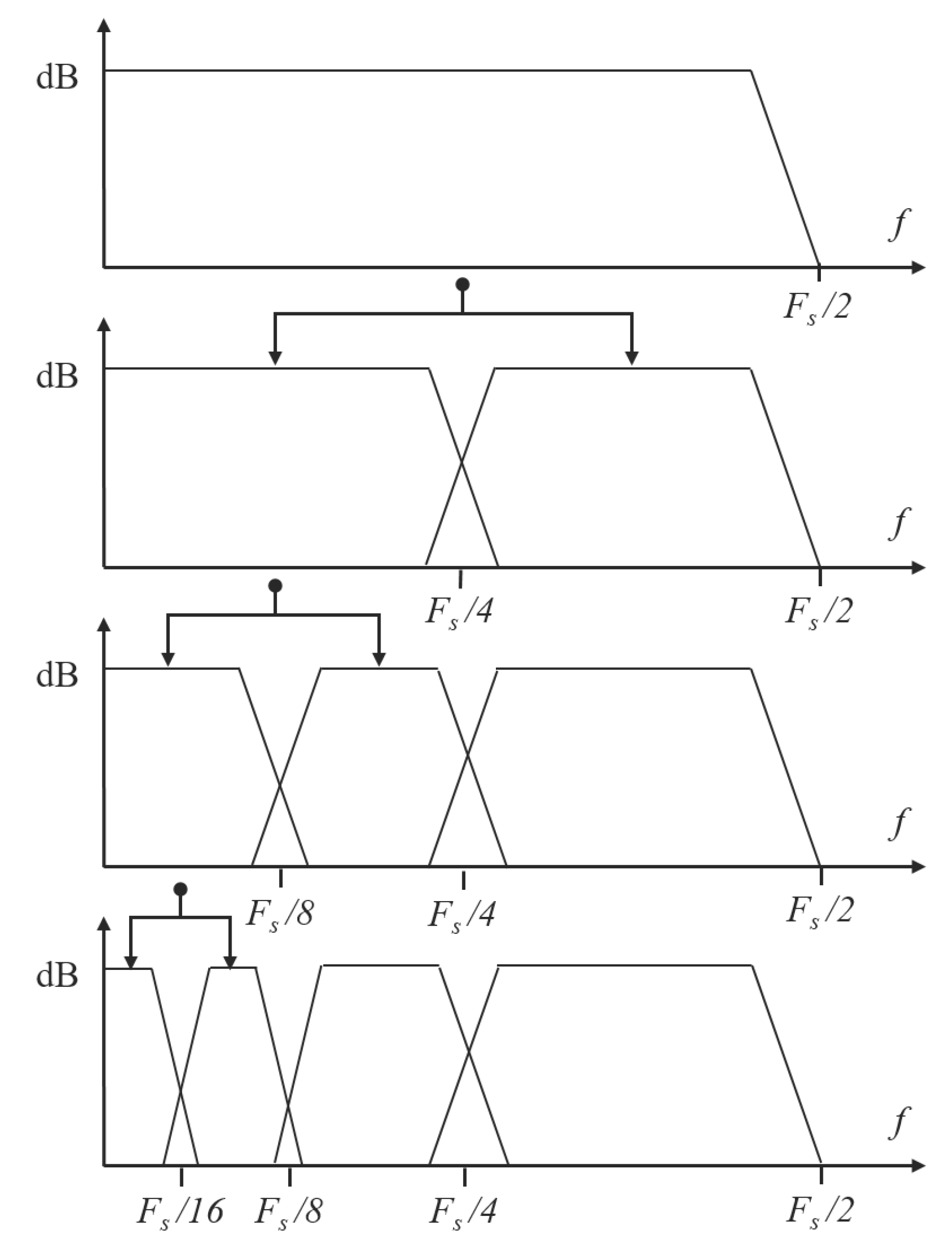
2.2. Wavelet Transform

To analyze time series signal, frequency analysis methods like Fourier transform (FT) have been widely used in plenty of research [24,25,26]. However, FT is weak in analyzing non-stationary signal because it represents only frequency domain [27]. Short-time Fourier transform (STFT), which is proposed to solve the problem, is used for analysis of non-stationary signals by windowing the signal using shifted window function [28]. Although the STFT has the advantage, it has weaknesses: (1) Dilemma of resolution, (2) Unchanged window, and (3) Heisenberg uncertainty principle [29,30]. Wavelet transform (WT) can be used to meet the above requirement. WT represents the signal in time and frequency domain and can change the frequency resolution and time interval by dilation and shift of wavelet function [31,32].

The wavelet function, ${\psi }_{(a,b)}\left(t\right)$, is derived from mother wavelet $\psi \left(t\right)$ by dilation and translation.

$${\psi }_{(a,b)}\left(t\right)=\frac{1}{\sqrt{a}}\psi \left(\frac{t-b}{a}\right)$$

(5)

where a is the scaling parameter which is inversely proportional to frequency, b is the time localization parameter, $a>0$ and $b\in \mathbb{R}$. The parameters make daughter wavelet function differ from others. The wavelet transform is performed by following equation:

$$\mathit{W}\left(a,b\right)=\frac{1}{\sqrt{a}}\int x\left(t\right){\psi }_{a,b}^{*}\left(t\right)dt$$

(6)

where ‘*’ denotes complex conjugation.

The discrete wavelet transform (DWT) is based on multiresolution analysis. The DWT divides signal into different frequency components. These components are precisely obtained by splitting with frequency bands of a signal into various sub-bands based on a power of two divisions, which is called dyadic sampling. Initially, the signal is split into two wavelet coefficient, one is approximation coefficient that is result of low-pass filter, and the other is detail coefficient that is result of high-pass filter. The approximation coefficient still has high-frequency components, so to continuously conduct the process is needed until getting useful feature as shown in Figure 3. $G_1\left(z\right)$ is high-pass filter and $G_0\left(z\right)$ is low-pass filter, after through filter the signal down-sampled as half. This process splits the discrete signal spectrum in the frequency domain as shown in Figure 4.

3. Data Description and Detection Index

This section describes the data of signal that is measured from CNC machine to help understanding for CNC machine signal and feature extraction.

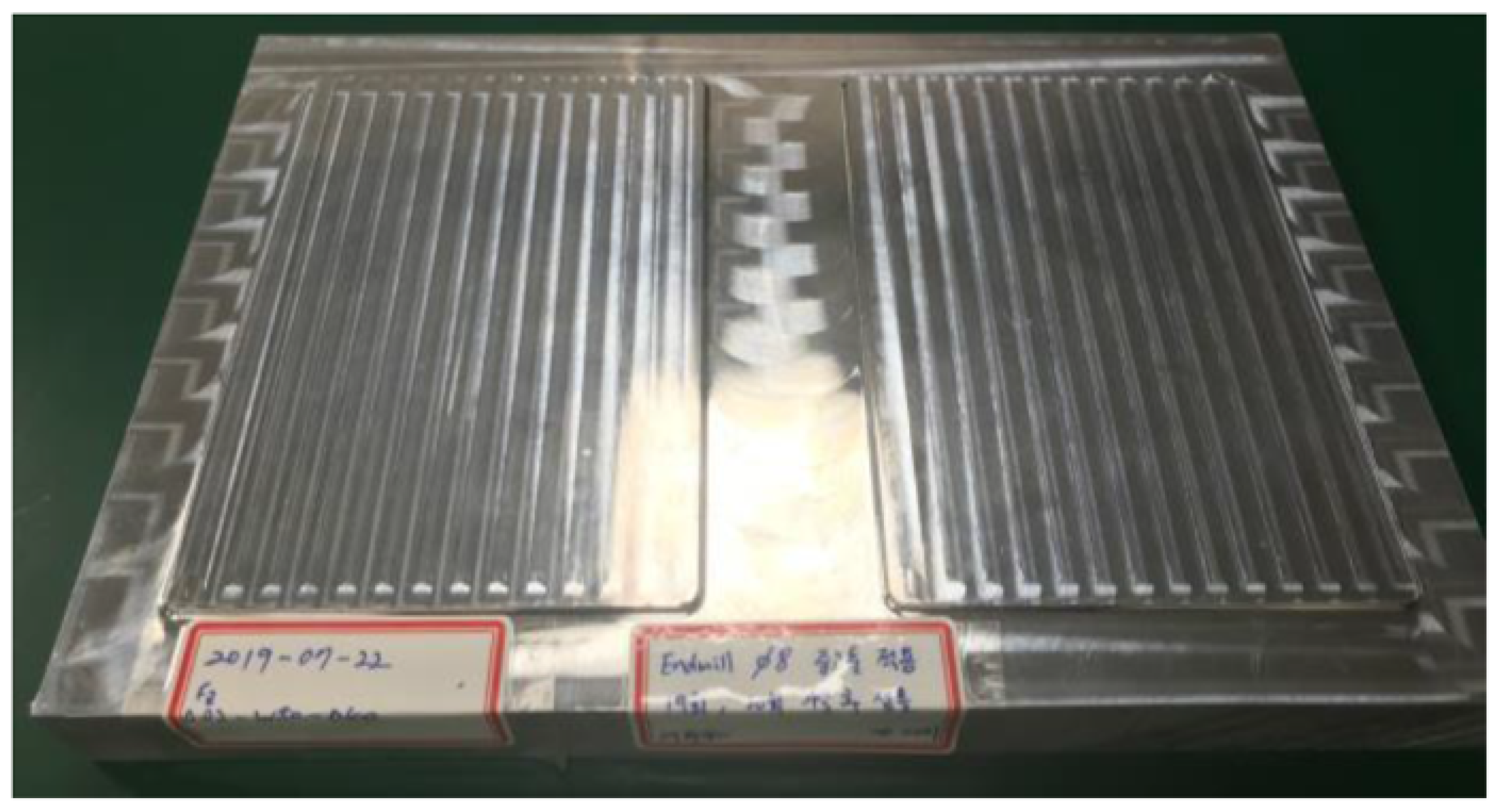
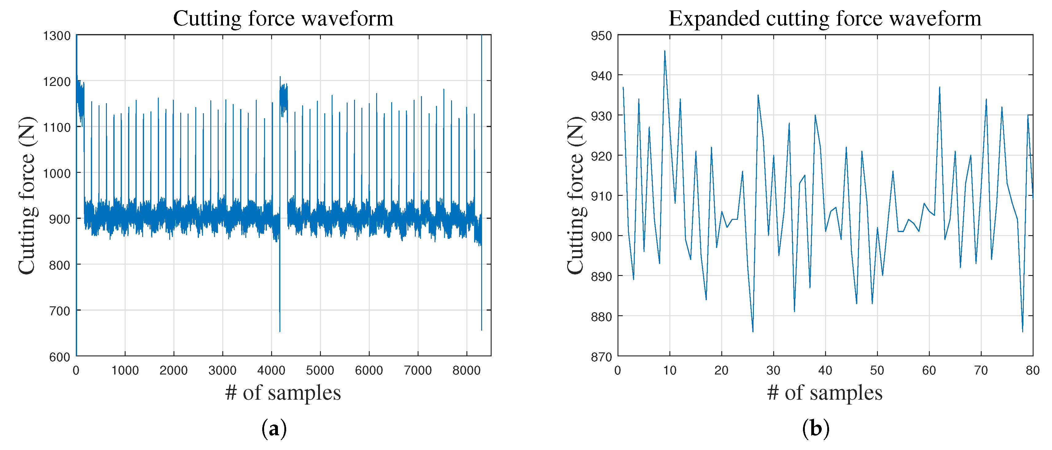
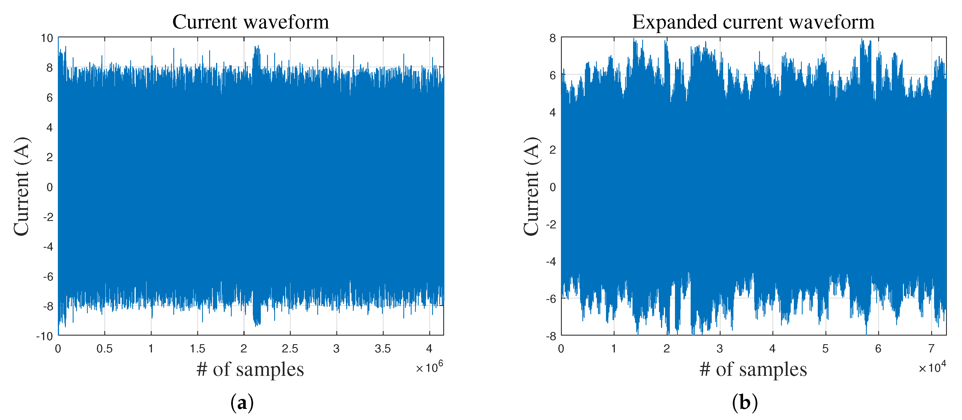
3.1. Data Description

CNC machine used in this paper is Dusan mynx 5400 as shown in Figure 5. We produced products like Figure 6 pattern. The tool size is $8\varphi$ and the tool has three blades.

In this paper, we use two types of sensor data, cutting force and current. Cutting force is measured from CNC machine and current is three-phase current measured from spindle motor. Current measurement device is designed and manufactured Korea electrotechnology research institute (KERI). Figure 7 and Figure 8 show cutting force and current waveform. In case of current waveforms, we only show u-phase waveform because others current show similar pattern.

Cutting force sampling time is 4 Hz and current sampling time is 2000 Hz. We synchronize current signal on the basis of cutting force signal, which has lower sampling frequency, because the sampling frequencies of two signal are differ. There are high impulse data in cutting force signal when the tool move next line. The impulse signal can interrupt tool diagnosis, hence the signal should be removed for good performance. The cutting force signal removed impulse signal is depicted in Figure 7b. After removing the impulse signal from the cutting force signal, we synchronize the current signal on the basis of the cutting force signal. Figure 8b shows the current signal that is equivalent to Figure 7b interval.

3.2. Feature Extraction

In this paper, we use three tool diagnosis models as shown in Figure 1. Among the models, Figure 1b,c models, which don’t use original signal of cutting force and current, uses feature of cutting force and current signal. Let $C{F}_{CNC}$ and $I_{phase}$ be cutting force and current signal, respectively. Three-phase current are divided as u, v, and w. These are indicated $I_u$, $I_v$, and $I_w$.

The features employed in this paper are mean, maximum, minimum, median, and standard deviation value in case cutting force. In case of current, RMS calculated by three-phase current is employed and maximum, standard deviation and RMS values calculated by each phase current are employed. The RMS about three-phase current is defined as [33]:

$$I_{RMS}=\sqrt{\frac{1}{3}\left(I_u^2+I_v^2+I_w^2\right)}$$

(7)

In this paper, we apply 6-level discrete wavelet transform to decompose the current signal that is high frequency signal and is measured by high sampling rate. Each signal derives six detail coefficients and an approximation coefficient. To extract feature from result of DWT, we calculate the using the derived signal. RMS of wavelet coefficient is defined as:

$$A_{RMS}=\frac{2}{F_s}\sum _k^{Fs/2}{A}_L^2\left(k\right)$$

(8)

$$D_{RMS}\left(l\right)=\frac{2k}{F_s}\sum _k^{F_s/2k}{D}_l^2\left(k\right)$$

(9)

where $A_{RMS}$, $D_{RMS}$, $A_L$, and $D_l$ are RMS value of approximation coefficient, detail coefficient, final level approximation coefficient and l-level detail coefficient, respectively. $F_s$ is sampling frequency, l indicates level of DWT.

Extracted features are totally 36 variables as shown in

Table 1. Feature variables extracted from cutting force and current signal.

Notation	Description	Unit	Notation	Description	Unit
$X_1$	Average of cutting force	N	$X_{19}$	RMS value of $D_4$ (v-phase)	-
$X_2$	Maximum value of cutting force	N	$X_{20}$	RMS value of $D_5$ (v-phase)	-
$X_3$	Minimum value of cutting force	N	$X_{21}$	RMS value of $D_6$ (v-phase)	-
$X_4$	Median of cutting force	N	$X_{22}$	RMS value of $A_6$ (v-phase)	-
$X_5$	STD of cutting force	N	$X_{23}$	RMS value of $D_1$ (u-phase)	-
$X_6$	RMS value of u-phase	A	$X_{24}$	RMS value of $D_2$ (u-phase)	-
$X_7$	Maximum value of u-phase	A	$X_{25}$	RMS value of $D_3$ (u-phase)	-
$X_8$	STD of u-phase	A	$X_{26}$	RMS value of $D_4$ (u-phase)	-
$X_9$	RMS value of v-phase	A	$X_{27}$	RMS value of $D_5$ (u-phase)	-
$X_{10}$	Maximum value of v-phase	A	$X_{28}$	RMS value of $D_6$ (u-phase)	-
$X_{11}$	STD of v-phase	A	$X_{29}$	RMS value of $A_6$ (u-phase)	-
$X_{12}$	RMS value of w-phase	A	$X_{30}$	RMS value of $D_1$ (w-phase)	-
$X_{13}$	Maximum value of w-phase	A	$X_{31}$	RMS value of $D_2$ (w-phase)	-
$X_{14}$	STD of w-phase	A	$X_{32}$	RMS value of $D_3$ (w-phase)	-
$X_{15}$	RMS value 3-phase	A	$X_{33}$	RMS value of $D_4$ (w-phase)	-
$X_{16}$	RMS value of $D_1$ (v-phase)	-	$X_{34}$	RMS value of $D_5$ (w-phase)	-
$X_{17}$	RMS value of $D_2$ (v-phase)	-	$X_{35}$	RMS value of $D_6$ (w-phase)	-
$X_{18}$	RMS value of $D_3$ (v-phase)	-	$X_{36}$	RMS value of $A_6$ (w-phase)	-

. The input vector $\mathbf{x}$ of tool diagnosis model employing feature variables uses these variables, so $\mathbf{x}\in {\mathbb{R}}^{36}$.

3.3. Detection Index

To diagnose CNC machine tool, residual vector ${\mathbf{e}}_{new}\left(k\right)\left(={\mathbf{x}}_{new}\left(k\right)-{\widehat{\mathbf{x}}}_{new}\left(k\right)\right)$ is calculated from original signal(${\mathbf{x}}_{new}\left(k\right)$) and estimated signal(${\widehat{\mathbf{x}}}_{new}\left(k\right)$) from auto-encoder model at sample k. After calculating residual vector, $SPE$ is applied for measuring magnitude of residual. $SPE$ is defined as:

$$\begin{array}{cc}\hfill \mathit{SPE}\left(k\right)& =∥{\mathbf{e}}_{\mathbf{new}}\left(k\right)∥\hfill \\ \hfill & ={\left({\mathbf{x}}_{new}\left(k\right)-{\widehat{\mathbf{x}}}_{new}\left(k\right)\right)}^T\left({\mathbf{x}}_{new}\left(k\right)-{\widehat{\mathbf{x}}}_{new}\left(k\right)\right)\hfill \end{array}$$

(10)

Tool condition is determined by $SPE$. The diagnosis model determine that tool is usable if $SPE$ is lower than a specific threshold value. On the other hands, if $SPE$ is higher than the threshold value, the diagnosis model determine that tool should be changed after some days or weeks. In this paper, we employ percentile and kernel density estimation for finding confidence limit used as threshold value.

4. Experiment and Discussion

4.1. Data Preparation

In this paper, we use two tools of CNC machine, a new tool and a used tool. The new tool has been used less than an hour and the use tool has been used over fifty hours. We made 4 workpieces with the new tool and 12 workpieces with the used tool. To generate the data which is able to apply to diagnosis models, we extract the part of signal processed in same pattern from the whole cutting force signal and remove the impulse signal which interrupt diagnosis. After extracting the cutting force signal, synchronizing the cutting force and the current signal should be performed because of different sampling time between the cutting force and the current signal. In the new tool dataset, there are 100 samples that are processed as same pattern. Among the new tool dataset, 80 samples are used as training dataset, others are employed test sample. In the used tool dataset, there are 218 samples that are processed as same pattern. Figure 1a model is trained by only the raw cutting force data in training dataset. Figure 1b,c models are trained by feature extracted from the cutting force and the current signal in training dataset. The cutting force and the feature data used as training and test data are normalized by the min-max normalization before training and test.

4.2. Experiments

In this paper, we experiment three models for diagnosis of CNC machine tool. Before training the test model is carried out, threshold value should be selected from detection index of training datasets. To select the threshold value, one-leave out method is employed [34]. The neural network and auto-encoder have different results even though the models have same structure and are trained by same datasets. Using this characteristic, we make 50 detection indices from different 50 models using a dataset for choosing the threshold value. Figure 9 shows the results of one-leave-out method as histogram, where dashed lines indicate threshold value which is 99 percent confidence level ($Th{r}_n$) of normal distribution, solid lines indicate threshold value which is 99 percentile($Th{r}_p$) value.

Model performance of auto-encoder indicates different results according to hyperparameter of auto-encoder (code size, the number of layers and the number of nodes per layer) and the number of learning epoch. Therefore, it is necessary for auto-encoder to optimize hyperparameter and the number of learning epoch. To optimize hyperparameter and the number of learning epoch, we carried out k-fold cross validation in this paper.

Table 2. Model hyperparameters and the number of learning epoch.

Model	Code Size	Number of Layers	Whole Structure	Learning Epoch
CFSAE	20	7	$80\times 60\times 30\times 20\times 30\times 60\times 80$	350
FSAE	10	7	$36\times 25\times 15\times 10\times 15\times 25\times 36$	200
FSAENR	10	7	$36\times 25\times 15\times 10\times 15\times 25\times 36$	200

indicates optimized hyperparameter and the number of learning epoch obtained through k-fold cross validation, where code size is the number of neurons in latent space (end of encoder). CFSAE, FAE and FSAENR are Figure 1a–c model, respectively. To verify the diagnosis models, we train the models according to optimized values. Figure 10 shows results of the diagnosis models. Figure 10a,c,e show $SPE$ result of each models. Blue solid line indicates calculation result of $SPE$ using the new tool data, black solid line is calculation result using the used tool. Blue and red dashed line indicate threshold value extracted from percentile and kernel density estimation results, respectively. Figure 10b,d,f indicate alarm signals. The alarm signals are divided as three cases: (1) Lower than both threshold values; (2) Intermediate value of both threshold values; (3) Higher than both threshold values.

In case of CFSAE, although $SPE$ of new tool do not exceed $Th{r}_p$, a lot of test cases exceed $Th{r}_n$. Moreover, the $SPE$s of new tool have similar value to $SPE$s of used tool. In case of FSAE and FSAENR, results of both models indicate similar waveform. However, FSAENR has a lot lower $SPE$ value than FASE since FSAENR calculates $SPE$ using normalized residual vector. Both models show properly classifying most case of test data.

Table 3. Performance of tool diagnosis models.

Model	$\mathit{SPE}<{\mathit{Thr}}_{\mathit{n}}$		${\mathit{Thr}}_{\mathit{n}}<\mathit{SPE}<{\mathit{Thr}}_{\mathit{n}}$		$\mathit{SPE}>{\mathit{Thr}}_{\mathit{p}}$		FNR (%)		FPR (%)
	New	Used	New	Used	New	Used	${\mathit{Thr}}_{\mathit{n}}$	${\mathit{Thr}}_{\mathit{p}}$	${\mathit{Thr}}_{\mathit{n}}$	${\mathit{Thr}}_{\mathit{p}}$
CFSAE	8	56	12	156	0	6	60.00	0.00	25.69	97.25
FSAE	14	0	6	1	0	217	30.00	0.00	0.00	0.46
FSAENR	16	0	4	1	0	217	20.00	0.00	0.00	0.46

show false negative rate (FNR, $\sum \left(Truenegative\right)/\sum \left(Conditionpositive\right)$) and false positive rate (FPR, $\sum \left(Truepositive\right)/\sum \left(Conditionnegative\right)$) of each model. Lower FNR means that the model has low type I error frequency and lower FPR means that the model has low type II error frequency.CFSAE model shows high FNR and FPR. FSAE and FSAENR show lower FNR and FPR. Furthermore, FSAENR model shows 10 percent lower FNR than FSAE.

5. Conclusions

In this paper, we proposed CNC tool diagnosis models using auto-encoder. The auto-encoder is unsupervised method which do not need labeled data, so the method is appropriate at processes that have difficult to get the plenty of failure data. We used the cutting force extracted from CNC machine and the current data extracted from spindle motor for machine tool diagnosis. The diagnosis model that had used raw data showed low performance. Hence, feature data generated from the cutting force and current signal are employed. We carried out experiments about three models. The CFSAE model used raw cutting force data. The FSAE and FSAENR models used feature data. The results of CFSAE showed that the new tool and the used tool have similar SPE value, so the CFSAE model have not identified the type of tools. Hence, FNR and FPR of CFSAE model is high. In case of FSAE and FSAENR models, the used tool signals were almost completely classified and the test cases of new tool are perfectly identified at using $Th{r}_p$ as threshold value, FNR is zero. It can be seen that the feature data represents the characteristics of fault signal better than the raw signal. Furthermore, FSAENR has lower FNR than FSAE since normalized residual vector reduce effect of large unit scale like cutting force signal.

The condition based maintenance needs not only fault detection and tool diagnosis but also prediction model which estimates remained life time of tool. In future work, we will research about the tool diagnosis model that can continuously update criteria of tool condition using cumulated data in online and prediction model that can estimate remained life time of tool and denote the time to replace tool.

References

1. Lauro, C.; Brandão, L.; Baldo, D.; Reis, R.; Davim, J. Monitoring and processing signal applied in machining processes—A review. Measurement 2014, 58, 73–86. [Google Scholar] [CrossRef]
2. Tobon-Mejia, D.; Medjaher, K.; Zerhouni, N. CNC machine tool’s wear diagnostic and prognostic by using dynamic Bayesian networks. Mech. Syst. Signal Process. 2012, 28, 167–182. [Google Scholar] [CrossRef] [Green Version]
3. Choudhary, A.; Goyal, D.; Shimi, S.L.; Akula, A. Condition monitoring and fault diagnosis of induction motors: A review. Arch. Comput. Methods Eng. 2019, 26, 1221–1238. [Google Scholar] [CrossRef]
4. Bassiuny, A.; Li, X. Flute breakage detection during end milling using Hilbert–Huang transform and smoothed nonlinear energy operator. Int. J. Mach. Tools Manuf. 2007, 47, 1011–1020. [Google Scholar] [CrossRef]
5. Reñones, A.; de Miguel, L.J.; Perán, J.R. Experimental analysis of change detection algorithms for multitooth machine tool fault detection. Mech. Syst. Signal Process. 2009, 23, 2320–2335. [Google Scholar] [CrossRef]
6. Ghosh, N.; Ravi, Y.; Patra, A.; Mukhopadhyay, S.; Paul, S.; Mohanty, A.; Chattopadhyay, A. Estimation of tool wear during CNC milling using neural network-based sensor fusion. Mech. Syst. Signal Process. 2007, 21, 466–479. [Google Scholar] [CrossRef]
7. Wang, G.; Zhang, Y.; Liu, C.; Xie, Q.; Xu, Y. A new tool wear monitoring method based on multi-scale PCA. J. Intell. Manuf. 2019, 30, 113–122. [Google Scholar] [CrossRef]
8. Luo, B.; Wang, H.; Liu, H.; Li, B.; Peng, F. Early fault detection of machine tools based on deep learning and dynamic identification. IEEE Trans. Ind. Electron. 2018, 66, 509–518. [Google Scholar] [CrossRef]
9. Glowacz, A. Fault detection of electric impact drills and coffee grinders using acoustic signals. Sensors 2019, 19, 269. [Google Scholar] [CrossRef] [Green Version]
10. Taghizadeh-Alisaraei, A.; Mahdavian, A. Fault detection of injectors in diesel engines using vibration time-frequency analysis. Appl. Acoust. 2019, 143, 48–58. [Google Scholar] [CrossRef]
11. Huang, S.; Tan, K.; Wong, Y.; De Silva, C.; Goh, H.; Tan, W. Tool wear detection and fault diagnosis based on cutting force monitoring. Int. J. Mach. Tools Manuf. 2007, 47, 444–451. [Google Scholar] [CrossRef]
12. Cai, B.; Zhao, Y.; Liu, H.; Xie, M. A data-driven fault diagnosis methodology in three-phase inverters for PMSM drive systems. IEEE Trans. Power Electron. 2016, 32, 5590–5600. [Google Scholar] [CrossRef]
13. Zhang, H.; Chen, H.; Guo, Y.; Wang, J.; Li, G.; Shen, L. Sensor fault detection and diagnosis for a water source heat pump air-conditioning system based on PCA and preprocessed by combined clustering. Appl. Therm. Eng. 2019, 160, 114098. [Google Scholar] [CrossRef]
14. Saari, J.; Strömbergsson, D.; Lundberg, J.; Thomson, A. Detection and identification of windmill bearing faults using a one-class support vector machine (SVM). Measurement 2019, 137, 287–301. [Google Scholar] [CrossRef]
15. Wang, X.; Ma, L.; Wang, T. An optimized nearest prototype classifier for power plant fault diagnosis using hybrid particle swarm optimization algorithm. Int. J. Electr. Power Energy Syst. 2014, 58, 257–265. [Google Scholar] [CrossRef]
16. Yu, J.; Jang, J.; Yoo, J.; Park, J.H.; Kim, S. A Clustering-Based Fault Detection Method for Steam Boiler Tube in Thermal Power Plant. J. Electr. Eng. Technol. 2016, 11, 848–859. [Google Scholar] [CrossRef] [Green Version]
17. Sun, M.; Wang, H.; Liu, P.; Huang, S.; Fan, P. A sparse stacked denoising autoencoder with optimized transfer learning applied to the fault diagnosis of rolling bearings. Measurement 2019, 146, 305–314. [Google Scholar] [CrossRef]
18. Yu, H.; Wang, K.; Li, Y.; Zhao, W. Representation Learning With Class Level Autoencoder for Intelligent Fault Diagnosis. IEEE Signal Process. Lett. 2019, 26, 1476–1480. [Google Scholar] [CrossRef]
19. Yin, C.; Zhang, S.; Wang, J.; Xiong, N.N. Anomaly Detection Based on Convolutional Recurrent Autoencoder for IoT Time Series. IEEE Trans. Syst. Man Cybern. Syst. 2020. [Google Scholar] [CrossRef]
20. Hung, C.W.; Li, W.T.; Mao, W.L.; Lee, P.C. Design of a Chamfering Tool Diagnosis System Using Autoencoder Learning Method. Energies 2019, 12, 3708. [Google Scholar] [CrossRef] [Green Version]
21. Jiang, G.; He, H.; Xie, P.; Tang, Y. Stacked multilevel-denoising autoencoders: A new representation learning approach for wind turbine gearbox fault diagnosis. IEEE Trans. Instrum. Meas. 2017, 66, 2391–2402. [Google Scholar] [CrossRef]
22. LeCun, Y.; Bengio, Y.; Hinton, G. Deep learning. Nature 2015, 521, 436–444. [Google Scholar] [CrossRef] [PubMed]
23. Liu, G.; Bao, H.; Han, B. A stacked autoencoder-based deep neural network for achieving gearbox fault diagnosis. Math. Probl. Eng. 2018, 2018, 5105709. [Google Scholar] [CrossRef] [Green Version]
24. Zhang, Z.; Wang, Y.; Wang, K. Fault diagnosis and prognosis using wavelet packet decomposition, Fourier transform and artificial neural network. J. Intell. Manuf. 2013, 24, 1213–1227. [Google Scholar] [CrossRef]
25. Rai, V.; Mohanty, A. Bearing fault diagnosis using FFT of intrinsic mode functions in Hilbert–Huang transform. Mech. Syst. Signal Process. 2007, 21, 2607–2615. [Google Scholar] [CrossRef]
26. Mark, S.; Sahu, R.; Kantarovich, K.; Podshyvalov, A.; Guterman, H.; Goldstein, J.; Jagannathan, R.; Mordechai, S. Fourier transform infrared microspectroscopy as a quantitative diagnostic tool for assignment of premalignancy grading in cervical neoplasia. J. Biomed. Opt. 2004, 9, 558–568. [Google Scholar] [CrossRef] [PubMed]
27. Lin, J.; Zuo, M. Gearbox fault diagnosis using adaptive wavelet filter. Mech. Syst. Signal Process. 2003, 17, 1259–1269. [Google Scholar] [CrossRef]
28. Singh, G.; Ahmed, S.A.K.S. Vibration signal analysis using wavelet transform for isolation and identification of electrical faults in induction machine. Electr. Power Syst. Res. 2004, 68, 119–136. [Google Scholar] [CrossRef]
29. Busch, P.; Heinonen, T.; Lahti, P. Heisenberg’s uncertainty principle. Phys. Rep. 2007, 452, 155–176. [Google Scholar] [CrossRef] [Green Version]
30. Percival, D.B.; Walden, A.T. Wavelet Methods for Time Series Analysis; Cambridge University Press: New York, NY, USA, 2000; Volume 4. [Google Scholar]
31. Sharma, M.; Achuth, P.V.; Deb, D.; Puthankattil, S.D.; Acharaya, U.R. An automated diagnosis of depression using three-channel bandwidth-duration localized wavelet filter bank with EEG signals. Cog. Syst. Res. 2018, 52, 508–520. [Google Scholar] [CrossRef]
32. Shah, S.; Sharma, M.; Deb, D.; Pachori, R.B. An automated alcoholism detection using orthogonal wavelet filter bank. In Machine Intelligence and Signal Analysis; Springer: Singapore, 2019; pp. 473–483. [Google Scholar]
33. Kia, S.H.; Henao, H.; Capolino, G.A. Diagnosis of broken-bar fault in induction machines using discrete wavelet transform without slip estimation. IEEE Trans. Ind. Appl. 2009, 45, 1395–1404. [Google Scholar] [CrossRef]
34. Han, J.; Pei, J.; Kamber, M. Data Mining: Concepts and Techniques; Morgan Kaufmann: Waltham, MA, USA, 2011. [Google Scholar]
Figure 1. Tool condition diagnosis models: (a) Cutting force based stacked auto-encoder; (b) Feature based stacked auto-encoder; (c) Feature based stacked auto-encoder using normalized residual vector.
Processes 08 00456 g001
Figure 2. Basic auto-encoder structure.
Processes 08 00456 g002
Figure 3. Discrete wavelet transform signal flow chart.
Processes 08 00456 g003
Figure 4. Signal split using discrete wavelet transform.
Processes 08 00456 g004
Figure 5. CNC machine: Dusan Mynx 5400.
Processes 08 00456 g005
Figure 6. Example products.
Processes 08 00456 g006
Figure 7. Cutting force signal waveform: (a) Entire data; (b) Part of signal that is removed impulse signal.
Processes 08 00456 g007
Figure 8. Current signal waveform: (a) Entire u-phase current data; (b) Part of signal that is equivalent to part of cutting force signal removed impulse signal.
Processes 08 00456 g008
Figure 9. Histogram of SPE results calculated from training dataset: (a) Results of CFSAE; (b) Results of FSAE; (c) Results of FSAENR.
Processes 08 00456 g009
Figure 10. Experimental results and alarm signal of each model: (a) SPE of CFSAE; (b) Alarm signal of CFSAE; (c) SPE of FSAE; (d) Alarm signal of FSAE; (e) SPE of FSAENR; (f) Alarm signal of FSAENR.
Processes 08 00456 g010