The Potential of Fractional Order Distributed MPC Applied to Steam/Water Loop in Large Scale Ships

Abstract

The steam/water loop is a crucial part of a steam power plant. However, satisfying control performance is difficult to obtain due to the frequent disturbance and load fluctuation. A fractional order model predictive control was studied in this paper to improve the control performance of the steam/water loop. Firstly, the dynamic of the steam/water loop was introduced in large-scale ships. Then, the model predictive control with an extended prediction self adaptive controller framework was designed for the steam/water loop with a distributed scheme. Instead of an integer cost function, a fractional order cost function was applied in the model predictive control optimization step. The superiority of the fractional order model predictive control was validated with reference tracking and load fluctuation experiments.

1. Introduction

A total of 80% trade volume is moved with shipping industry, which is becoming an important part of the world economy [1]. In order to obtain large carrying capacity and low operation cost, there is a large demand for large-scale cargo ships. To achieve energy saving and a stable energy supply, research is required to optimize the power plant in large-scale ships [2]. The steam/water loop in large scale ships has the function of supplying water and recovering the waste steam for the steam power plant. There are five output variables including the drum water level, exhaust manifold pressure, deaerator pressure, deaerator water level and condenser water level. The steam/water loop has the features of nonlinearity, multi variables and strong coupling system. During the operating of the ship, the frequent disturbance and load fluctuation make it difficult to obtain a satisfying control effect for the five sub-loops [3]. The challenges in the control of steam/water loop can be summarized as follows:

• the steam/water loop is a system of nonlinearity, strong interactions and multivariable;
• load and disturbances change frequently with large amplitude;
• operating conditions changes frequently (there are ten levels of the sea state);
• demands for mobility and rapidity are growing high.

The Model Predictive Control (MPC) is a widely applied controller in industrial processes for its ability to deal with constraints such as the input saturation and rate limits. The dynamic model of the system is required to predict and optimize the future error and control effort by minimizing a cost function [4]. MPC has become the mostly applied control strategy in a wide variety of areas, including petroleum, refining and chemical industries [5]. Part of the work about the application of MPC to the boiler system is shown in [6,7,8]. In the cost function, an economic index was included [6]. The reference tracking and the economic performance were both realized. To realize satisfying control performance for ultra-supercritical boiler, a fuzzy model was obtained for the fuzzy MPC, and a linear extended state observer was improved to estimate plant behavior variations and unknown disturbances [7]. A state-space model was linearized on-line to improve the computationally efficient in model predictive control, and the results were similar to the results obtained with nonlinear model [8]. For tuning the closed loops with MPC, a practical method with step response of the system was proposed [9]. The methodology is suitable for hands-on tuning of MPC. Compared with PID control, it is discussed about when, where and why to apply the MPC with the advent of Industry 4.0 [10].

The fractional order calculus has attracted increasing attention over the past two decades for its versatility in modeling and control applications [11]. Although the computational load will increase with fractional order, nowadays, the development of microprocessor makes it possible for such kind of computation. Some types of control strategies have been generalized with fractional order calculus [12,13]. For example, the PID controller is the most used in industry [14], hence, fractional order calculation was added to PID controller in many applications such as: AR.Drone quad-rotor [15], induction motor drive system [16], multi-area interconnected power systems [17], heterogeneous dynamic systems [18], automatic regulator voltage system [19], multiple UAVs formation [20,21], velocity control system [22]. The fractional order calculus is also applied in the MPC method. And the application can be found such as temperature control [23], and frequency control of an islanded micro-grid [24].

In the fractional order calculus, ${}_a{D}_b^{\alpha }$ is commonly used for $\alpha$-th order derivative in the interval [a, b], and ${}_a{I}_b^{\alpha }$ the $\alpha$-th fractional order integral in the interval [a, b]. There are two kinds of approximate estimators for the fractional calculus. One is the Grünwald-Letnikov (GL) definition, and another Riemann-Liouville (RL) definition. The RL definition is used for continuous domain, while GL definition for numerical integration and simulation purposes. Their definitions are

$${}_a{D}_t^{\alpha }f{\left(t\right)}_{t=k{T}_s}=\underset{T_s\to 0}{lim}{T_s}^{-\alpha }\sum _{i=0}^{\left[\frac{t-a}{T_s}\right]}{(-1)}^i\left(\begin{array}{c}\alpha \\ i\end{array}\right)f(k{T}_s-i{T}_s)\mathbf{GL}$$

(1)

$${}_a{D}_t^{\alpha }f\left(t\right)=\frac{1}{\mathrm{\Gamma }(n-\alpha )}\frac{d^n}{d{t}^n}{\int }_a^t\frac{f\left(\tau \right)}{{(t-\tau )}^{(\alpha -n+1)}}d\tau \mathbf{RL}$$

(2)

where $T_s$ is the sampling time and $\mathrm{\Gamma }(·)$ is Euler’s Gamma function.

In this paper, the original contribution lies in that the constant values of the weighting factors in classical MPC is replaced with time-varying weighting factors in fractional order MPC (FOMPC). The weight factors in the classical MPC have $N_p+N_c$ elements for tracking error and control effort need to be defined, where $N_p$ is prediction horizon and $N_c$ is control horizon. The optimal problem for the weighting factors will be very complex. Hence, the weighting factors are mostly kept as constants in MPC. In the FOMPC, the weighting factors are obtained with the fractional orders, in which optimal different weighting factors can be tuned with two fractional orders, one for the tracking error and another for control effort. Hence, the FOMPC will result in a better system performance than the MPC method. In this work, fractional order MPC is proposed firstly for steam/water loop with GL definition. Then, the integer order cost function is replaced with a fractional order one in the MPC. In order to obtain a relatively good value set for the five sub-loops, different fractional orders are required for each sub-loop. The results show that the bigger fractional order leads to better control performance. Finally, reference tracking and load fluctuation experiments are conducted to verify the effectiveness of the FOMPC.

The paper is structured as follows: firstly, the steam/water loop is introduced in Section 2. Section 3 gives a brief introduction about Extended Prediction Self Adaptive Controller (EPSAC), and the fractional order cost function is designed. Section 4 shows the results of FOMPC compared with classical MPC. Conclusions are discussed in Section 5.

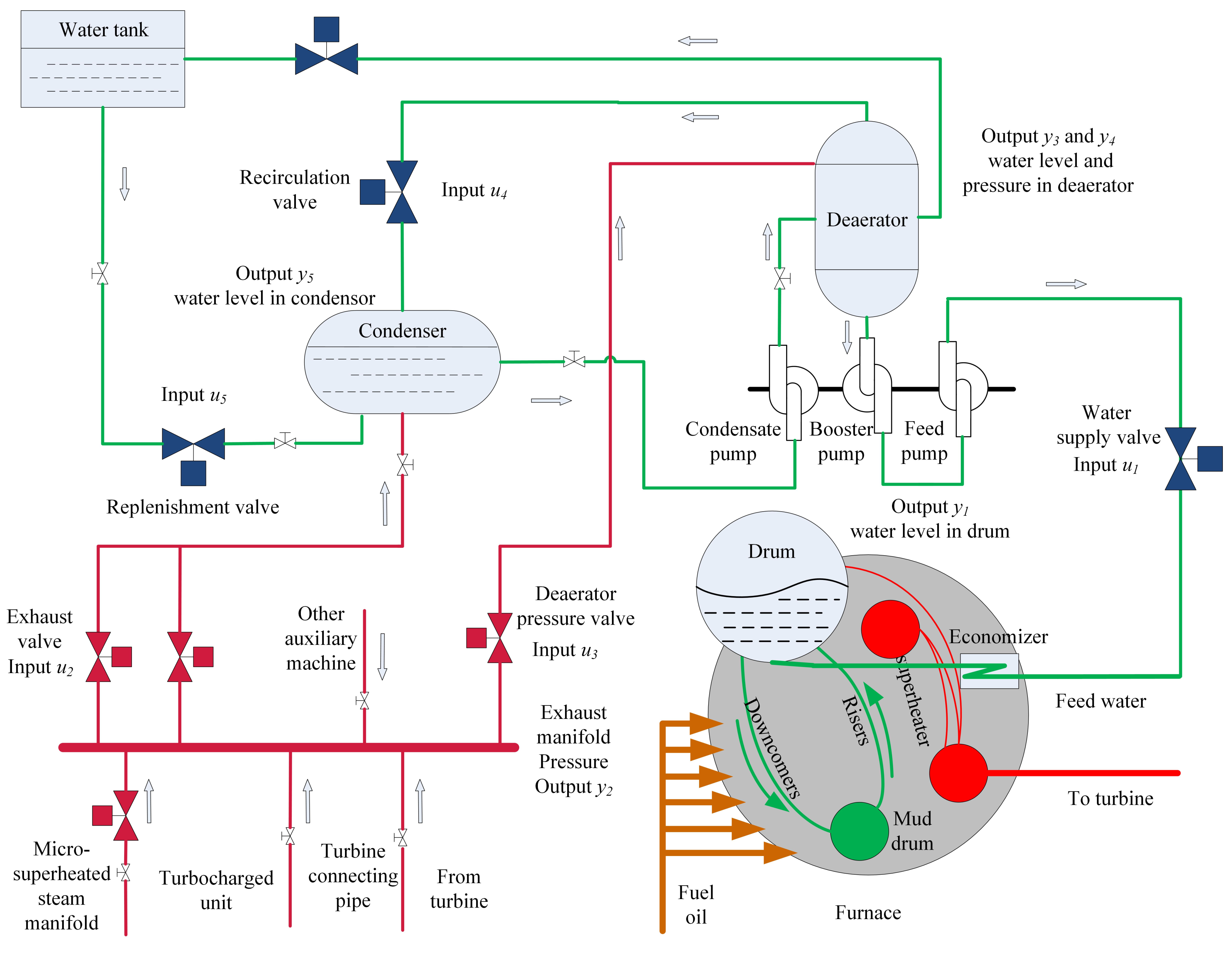
2. The Description for Steam/Water Loop

The steam/water loop in the large scale ships plays the role of supplying water to the boiler and recycling waste steam from turbine. The system is composed of a boiler drum, exhaust manifold, deaerator and condenser. The system operating principle can be found in Figure 1, in which there are two main operating loops. One is indicated with the red line for the steam loop, while the green line for the water loop. The description for the system are as follows: firstly, the condensed water from condenser goes to the deaerator for preheating and deoxygenation. Secondly, the feedwater is pumped to the drum. Due to the high density of the water than the steam, the water goes to the mud-drum. In the risers, the water absorbs the heat and becomes the mixture of steam and water. The steam gets separated in the drum and goes to the turbine after being heated in the economizer. The waste steam from the turbine and other auxiliary machines goes to the exhaust manifold. Most of the waste steam goes to the condenser, and the left part of waste steam goes to the deaerator for deoxygenation. Finally, the condensate water goes to the deaerator to work again.

In the steam/water loop, the input variables $\mathbf{u}=[u_1,u_2,\dots ,u_5]$ are valves for the five sub-loops, and the output variables $\mathbf{y}=[y_1,y_2,\dots ,y_5]$ are the drum water level ($y_1$), exhaust manifold pressure ($y_2$), deaerator pressure ($y_3$), deaerator water level ($y_4$), and condenser water level ($y_5$), respectively [3]. The transfer functions and constraints of the steam/water loop are shown as follows:

$$\left[\begin{array}{c}{y}_1\\ y_2\\ ⋮\\ y_5\end{array}\right]=\left[\begin{array}{cccc}{G}_{11}& G_{12}& \cdots & G_{15}\\ G_{21}& G_{22}& \cdots & G_{25}\\ ⋮& ⋮& \ddots & ⋮\\ G_{51}& G_{52}& \cdots & G_{55}\end{array}\right]\left[\begin{array}{c}{u}_1\\ u_2\\ ⋮\\ u_5\end{array}\right]$$

(3)

where $G_{11}=\frac{0.0000987}{(s+0.1131)(s+0.0085+0.032j)(s+0.0085-0.032j)}$, $G_{22}=\frac{0.7254}{(s+1.2497)(s+0.0223)}$, $G_{23}=\frac{-0.5}{(s+1.9747)(s+0.0253)}$, $G_{33}=\frac{0.0132}{(s+0.0265+0.0244j)(s+0.0265-0.0244j)}$, $G_{34}=\frac{-0.009}{(s+0.0997)(s+0.0411)}$, $G_{41}=\frac{-0.0008}{(s+0.012+0.126j)(s+0.012-0.126j)}$, $G_{44}=\frac{0.0005152}{(s+0.012+0.038j)(s+0.012-0.038j)}$, $G_{54}=\frac{-0.00015}{(s+0.0175+0.0179j)(s+0.0175-0.0179j)}$, $G_{55}=\frac{0.00147}{(s+0.025+0.0654j)(s+0.025-0.0654j)}$, and other transfer functions $G_{12}=G_{13}=\dots =G_{53}=0$.

$$\left\{\begin{array}{c}{\displaystyle -0.007/s\le \frac{d{u}_1}{dt}\le 0.007/s0\le u_1\le 1}\hfill \\ {\displaystyle -0.01/s\le \frac{d{u}_2}{dt}\le 0.01/s0\le u_2\le 1}\hfill \\ {\displaystyle -0.01/s\le \frac{d{u}_3}{dt}\le 0.01/s0\le u_3\le 1}\hfill \\ {\displaystyle -0.007/s\le \frac{d{u}_4}{dt}\le 0.007/s0\le u_4\le 1}\hfill \\ {\displaystyle -0.007/s\le \frac{d{u}_5}{dt}\le 0.007/s0\le u_5\le 1}\hfill \end{array}\right.$$

(4)

The operating point and ranges of variables are shown in

Table 1. The operating points and range of the steam/water loop.

Outputs	Operating Points	Range	Units
Water level in drum	1.79	[1.39–2.19]	m
Pressure in exhaust manifold	100.03	[87.03–133.8]	MPa
Pressure in deaerator	30	[24.9–43.86]	KPa
Water level in deaerator	0.7	[0.49–0.89]	m
Water level in condenser	0.5	[0.32–0.63]	m

.

3. Fractional Order MPC with EPSAC Framework

3.1. Brief Introduction for EPSAC

In this part, a brief introduction about EPSAC is given, and the detailed theory is introduced in [26]. For a discrete system:

$$y\left(t\right)=x\left(t\right)+w\left(t\right)$$

(5)

where t is the discrete time index; $y\left(t\right)$ and $x\left(t\right)$ are the system output and model output, respectively; and $w\left(t\right)$ indicates the disturbance. The model output $x\left(t\right)$ can be obtained according to the system model and past model outputs and inputs:

$$x\left(t\right)=f\left[x\right(t-1),x(t-2),\dots ,u(t-1),u(t-2),\dots ]$$

(6)

The following two parts compose the future input in EPSAC:

$$u(t+k|t)=u_{base}(t+k|t)+\delta u(t+k|t)$$

(7)

where the $u_{base}(t+k|t)$ indicates the basic future control actions and $\delta u(t+k|t)$ is the optimized future control actions. With these two parts of future input, the predicted future system output can be divided with the following two parts:

$$y(t+k|t)=y_{base}(t+k|t)+y_{opt}(t+k|t)$$

(8)

where $y_{base}(t+k|t)$ is produced with the basic future control action $u_{base}(t+k|t)$ and $y_{opt}(t+k|t)$ is obtained with optimized future control action $\delta u(t+k|t)$. According to the discrete input scenario, the $y_{opt}(t+k|t)$ can be obtained with:

$$y_{opt}(t+k|t)=h_k\delta u\left(t\right|t)+h_{k-1}\delta u(t+1|t)+\dots +g_{k-N_c+1}\delta u(t+N_c-1|t)$$

(9)

where the $h_i$ and $g_i$ are the impulse response and step response coefficients of the system; $N_c$ is the control horizon and $N_p$ the prediction horizon. The system output can be re-written as:

$$\mathbf{Y}=\overline{\mathbf{Y}}+\mathbf{G}\mathbf{U}$$

(10)

with $\mathbf{Y}={[y(t+N_1|t)\dots y(t+N_p|t)]}^T$, $\mathbf{U}={[\delta u\left(t\right|t)\dots \delta u(t+N_c-1|t)]}^T$, $\overline{\mathbf{Y}}={[y_{base}(t+N_1|t)\dots y_{base}(t+N_P|t)]}^T$, and

$$\mathbf{G}=\left[\begin{array}{cccc}{h}_{N_1}& h_{N_1-1}& \dots & g_{N_1-N_c+1}\\ h_{N_1+1}& h_{N_1}& \dots & \dots \\ \dots & \dots & \dots & \dots \\ h_{N_P}& h_{N_P-1}& \dots & g_{N_P-N_c+1}\end{array}\right]$$

where $N_1$ is the time delay of the system.

The disturbance term $w\left(t\right)$ in Equation (5) is taken as a filtered white noise [26], which is given by:

$$w(t+k|t)=\frac{C\left(q^{-1}\right)}{D\left(q^{-1}\right)}{w}_f(t+k|t)$$

(11)

where $q^{-1}$ is the backward shift operator; $D\left(q^{-1}\right)=(1-q^{-1})A\left(q^{-1}\right)$; and $A\left(q^{-1}\right)$, $C\left(q^{-1}\right)$ are polynomials from Controlled Auto-Regressive Integrated Moving Average (CARIMA) model.

The cost function gives:

$$J_{MPC}=\sum _{k=N_1}^{N_p}{p}_k{[r(t+k|t)-y(t+k|t)]}^2+\sum _{k=1}^{N_u}{q}_k▵u{(t+k)}^2$$

(12)

where $p_k$ and $q_k$ are nonnegative weighting factors, which are kept as constants.

Rewrite the Equation (12) into matrix form, and the following can be obtained:

$$J_{MPC}={(\mathbf{R}-\mathbf{Y})}^T\mathbf{P}(\mathbf{R}-\mathbf{Y})+{\mathbf{U}}^T\mathbf{Q}\mathbf{U}={(\mathbf{R}-\overline{\mathbf{Y}}-\mathbf{GU})}^T\mathbf{P}(\mathbf{R}-\overline{\mathbf{Y}}-\mathbf{GU})+{\mathbf{U}}^T\mathbf{Q}\mathbf{U}$$

(13)

where $P=diag(p_1,p_2,\dots ,p_{(N_p-N_1+1)})$ and $Q=diag(q_1,q_2,\dots ,q_{N_u})$.

If there are constraints in the optimization problem, it can be solved with quadratic programming. Without constraints, the optimal input sequence for $\delta u(t+k|t)$ gives:

$${\mathbf{U}}_{\mathbf{MPC}}^{*}={({\mathbf{G}}^T\mathbf{P}\mathbf{G}+\mathbf{Q})}^{-1}{\mathbf{G}}^T\mathbf{P}(\mathbf{R}-\overline{\mathbf{Y}})$$

(14)

For the fractional order MPC, the cost function can be expressed with

$$J_{FOMPC}{=}^{\gamma }{I}_{N_1}^{N_p}{p}_k{[r(t+k|t)-y(t+k|t)]}^2{+}^{\lambda }{I}_1^{N_c}{q}_k▵u{(t+k)}^2$$

(15)

where [$N_1$, $N_p$] and [1, $N_c$] are the integration intervals, and ${}^{\gamma }{I}_{N_1}^{N_p}$ and ${}^{\lambda }{I}_1^{N_c}$ are the symbols for fractional order integral with $\gamma$ and $\lambda$ the fractional orders. The ${}^{\gamma }{I}_{N_1}^{N_p}$ and ${}^{\lambda }{I}_1^{N_c}$ can be rewritten as:

$$\begin{array}{cc}\hfill {}^{\gamma }{I}_{N_1}^{N_p}{p}_k{[r(t+k|t)-y(t+k|t)]}^2& ={\int }_{N_1}^{N_p}{D}^{1-\gamma }{p}_k{[r(t+k|t)-y(t+k|t)]}^{2}dt\hfill \\ \hfill {}^{\lambda }{I}_1^{N_c}{q}_k▵u{(t+k)}^2& ={\int }_{N_1}^{N_c}{D}^{1-\lambda }{q}_k▵u{(t+k)}^{2}dt\hfill \end{array}$$

(16)

According to [27], the Equation (15) can be approximated by:

$$\begin{array}{cc}\hfill J_{FOMPC}& ={(\mathbf{R}-\mathbf{Y})}^T\mathbf{P}\mathrm{\Gamma }(T_s,\gamma )(\mathbf{R}-\mathbf{Y})+{\mathbf{U}}^T\mathbf{Q}\mathrm{\Lambda }(T_s,\lambda )\mathbf{U}\hfill \\ \hfill & ={(\mathbf{R}-\overline{\mathbf{Y}}-\mathbf{GU})}^T\mathbf{P}\mathrm{\Gamma }(T_s,\gamma )(\mathbf{R}-\overline{\mathbf{Y}}-\mathbf{GU})+{\mathbf{U}}^T\mathbf{Q}\mathrm{\Lambda }(T_s,\lambda )\mathbf{U}\hfill \end{array}$$

(17)

$$\mathrm{\Gamma }(T_s,\gamma )=T_s^{\gamma }diag(m_{N_p-N_1},m_{N_p-N_1-1},\dots ,m_1,m_0)$$

(18)

$$\mathrm{\Lambda }(T_s,\lambda )=T_s^{\lambda }diag(m_{N_c},m_{N_c-1},\dots ,m_1,m_0)$$

(19)

The $m_i$ with fractional order $\alpha$ gives:

$$m_j={\omega }_j^{(-\alpha )}-{\omega }_{j-n}^{(-\alpha )}$$

(20)

where n is the number of the $m_i$.

$${\omega }_j^{-\alpha }=\left\{\begin{array}{c}(1-(1-\alpha )/j){\omega }_{j-1}^{(-\alpha )}j>0;\\ 1j=0;\\ 0j<0.\end{array}\right.$$

(21)

From Equation (18) to Equation (21), the weight matrix can be easily tuned with fractional order $\gamma$ and $\lambda$ in the cost function $J_{FOMPC}$. And the weighting factors in the FOMPC are time-varying along the prediction horizon and control horizon. If there are constraints, the optimization problem can be solved with quadratic programming. Without constraints, the optimal input sequence for $\delta u(t+k|t)$ in FOMPC can be obtained as:

$${\mathbf{U}}_{\mathbf{FOMPC}}^{*}={({\mathbf{G}}^T\mathbf{P}(\mathrm{\Gamma }+{\mathrm{\Gamma }}^{\mathbf{T}})\mathbf{G}+\mathbf{Q}(\mathrm{\Lambda }+{\mathrm{\Lambda }}^{\mathbf{T}}))}^{-1}{\mathbf{G}}^T\mathbf{P}(\mathrm{\Gamma }+{\mathrm{\Gamma }}^{\mathbf{T}})(\mathbf{R}-\overline{\mathbf{Y}})$$

(22)

3.2. Applied the EPSAC to the MIMO System with Distributed Scheme

Due to the flexibility and robustness of the distributed control, the EPSAC is applied to the steam/water loop in distributed scheme, in which each sub-loop works as independent modules with communication network. The application of distributed fractional order MPC on the steam/water loop is similar to the method introduced in [3], and the integer cost function is replaced with fractional order cost function. Only a brief introduction is given here about the distributed MPC.

In the distributed MPC, the inference from other sub-loops should be considered to optimize the future error and control effort for sub-loop i, hence, the item $\mathbf{GU}$ in Equations (13) and (17) should be replaced with ${\displaystyle \sum _{j=1}^5}{\mathbf{G}}_{ij}{\mathbf{U}}_j$, and ${\mathbf{G}}_{ij}$ is the transfer function of $i^{th}$ output from $j^{th}$ input. A pseudo-code for the distributed MPC is provided in Algorithm 1.

Algorithm 1: The iterative DiMPC

1: Sub-loop i receives an optimal local control action $\delta {\mathbf{U}}_i$ at the iterative time as $iter=0$ according to the EPSAC, and the local control action $\delta {\mathbf{U}}_i$ can be marked as $\delta {\mathbf{U}}_i^{iter}$, where $\delta {\mathbf{U}}_i$ indicates the vector of the optimizing future control actions with length of $N_{ci}$;    2: The $\delta {\mathbf{U}}_j^{iter}$ ($j\in N_i$, $N_i=\{j\in N:{\mathbf{G}}_{ij}\ne 0\}$) will be communicated with the loop i, and the $\delta {\mathbf{U}}_i^{iter+1}$ will be calculated again with the $\delta {\mathbf{U}}_j^{iter}$ from other loops;    3: If one of the termination conditions is reached, the $\delta {\mathbf{U}}_i^{iter+1}$ will be adopted to the system. Otherwise, the $iter$ will be set as $iter=iter+1$, and return to Step 2. The termination condition is shown as follows: $\left(\right||\delta {\mathbf{U}}_i^{iter+1}-\delta {\mathbf{U}}_i^{iter}\left|\right|⩽{\epsilon }_i)\vee (iter+1>\overline{iter})$, where $\epsilon$ is a positive constant and $\overline{iter}$ indicates the upper bound of the number of iteration times.    4: Calculate the optimal control effort as ${\mathbf{U}}_t={\mathbf{U}}_{base}+\delta {\mathbf{U}}^{iter}$, and the control effort will be applied to the system;    5: Set $t=t+1$, return to Step 1.

4. Results and Discussion

In this paper, reference tracking and load fluctuation experiments are conducted to verify the effectiveness of the FOMPC. The parameter configuration is listed in

Table 2. MPC parameters.

Parameters	${\mathit{N}}_{\mathit{c}}$	${\mathit{T}}_{\mathit{s}}$	${\mathit{N}}_{\mathit{p}}$	${\mathit{N}}_1$	${\mathit{N}}_{\mathit{s}}$
Values	$N_{c1}=4$, $N_{c2}=1$, $N_{c3}=1$, $N_{c4}=4$, $N_{c5}=6$ samples	$5s$	$N_{p1}=20$, $N_{p2}=15$, $N_{p3}=15$, $N_{p4}=20$, $N_{p5}=20$ samples	1	300

.

where, $N_s$ is the number of samples. The termination conditions for the distributed MPC are set as: (i) $\left|\right|\delta {\mathbf{U}}_i^{iter+1}-\delta {\mathbf{U}}_i^{iter}\left|\right|⩽0.002$; (ii) $iter>5$.

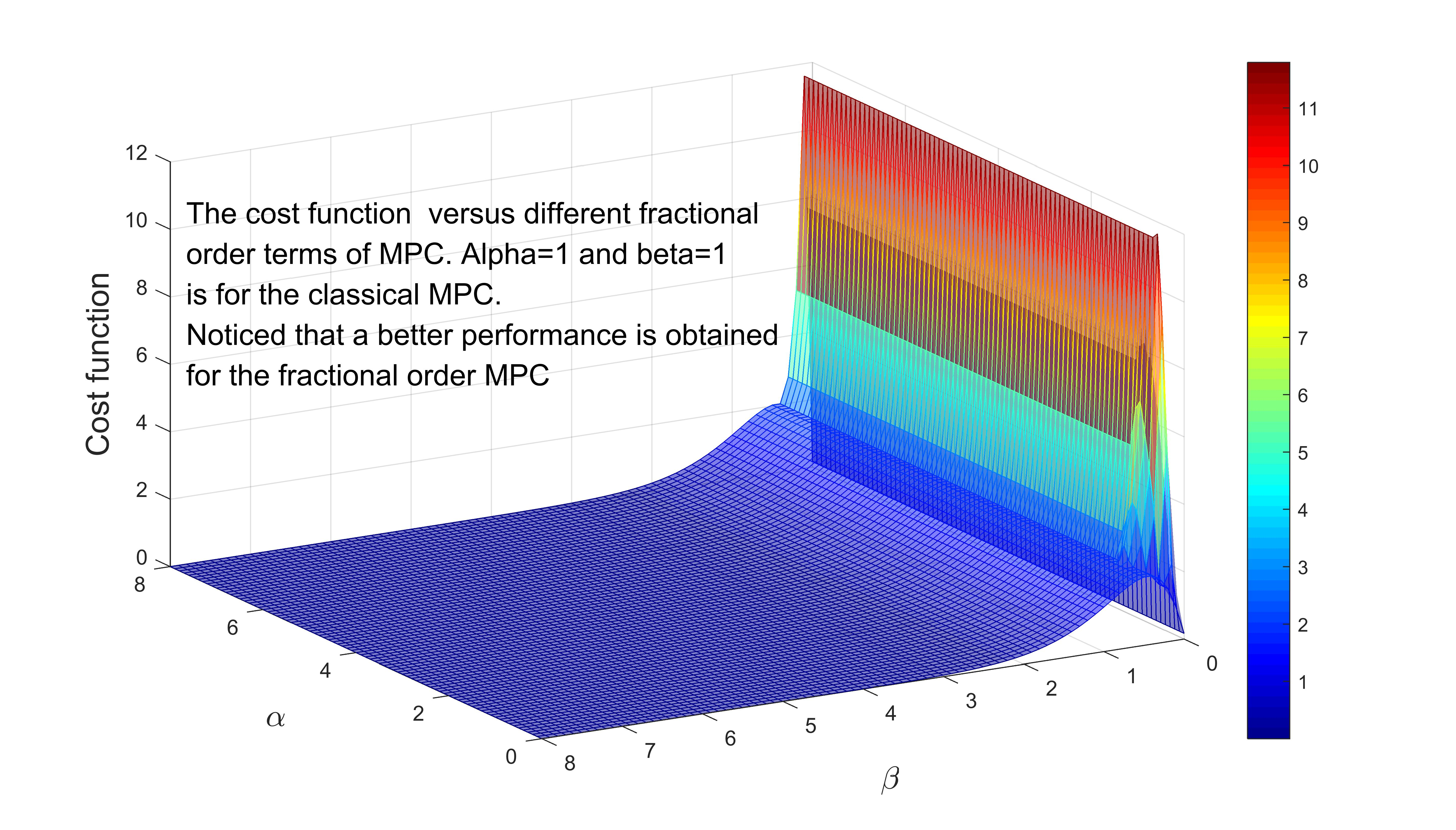
4.1. The Effect of Different Fractional Orders on the Overall System Performance

The choice of fractional orders of $\gamma$ and $\lambda$ have important influence on the system. To explore the effect of different fractional orders, the fractional orders listed in

Table 3. Different fractional orders for the five sub-loops.

Loops	Fractional Orders
Drum water level control loop	[6.2 5.0 3.8 2.6 1.0 0.8]
Exhaust manifold pressure control loop	[1.2 1.0 0.9 0.62 0.36 0.12]
Deaerator pressure control loop	[5.0 3.8 2.2 1.4 1.0 0.6]
Deaerator water level control loop	[1.5 1.2 1.0 0.8 0.4]
Condenser water level control loop	[2.2 1.8 1.2 1.0 0.7 0.3]

are applied for each sub-loop.

Intuitively from the results shown in Figure 2, all the outputs of the five sub-loops indicate that the larger fractional order leads to better responses both in response time and overshoot in a certain range. Also, the overshoot reduces with large fractional order value.

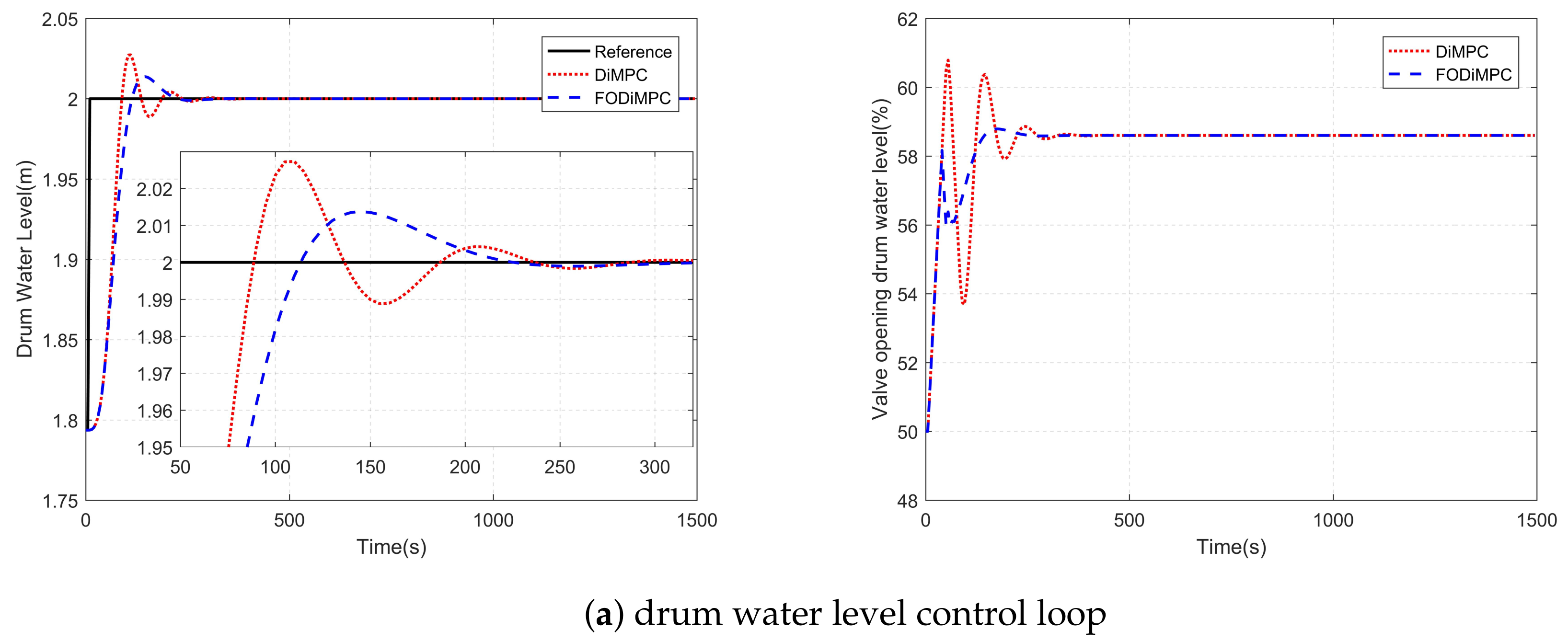
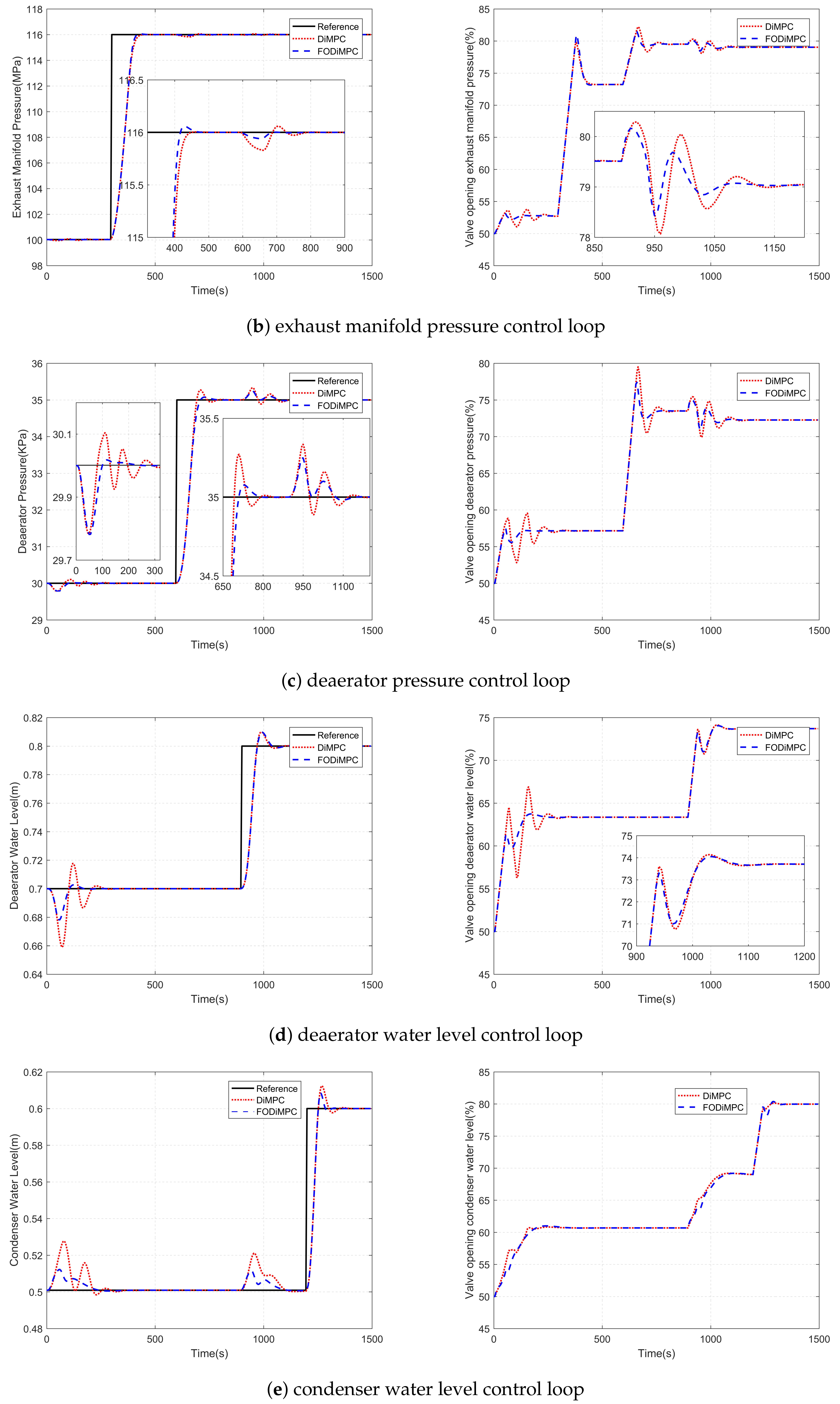
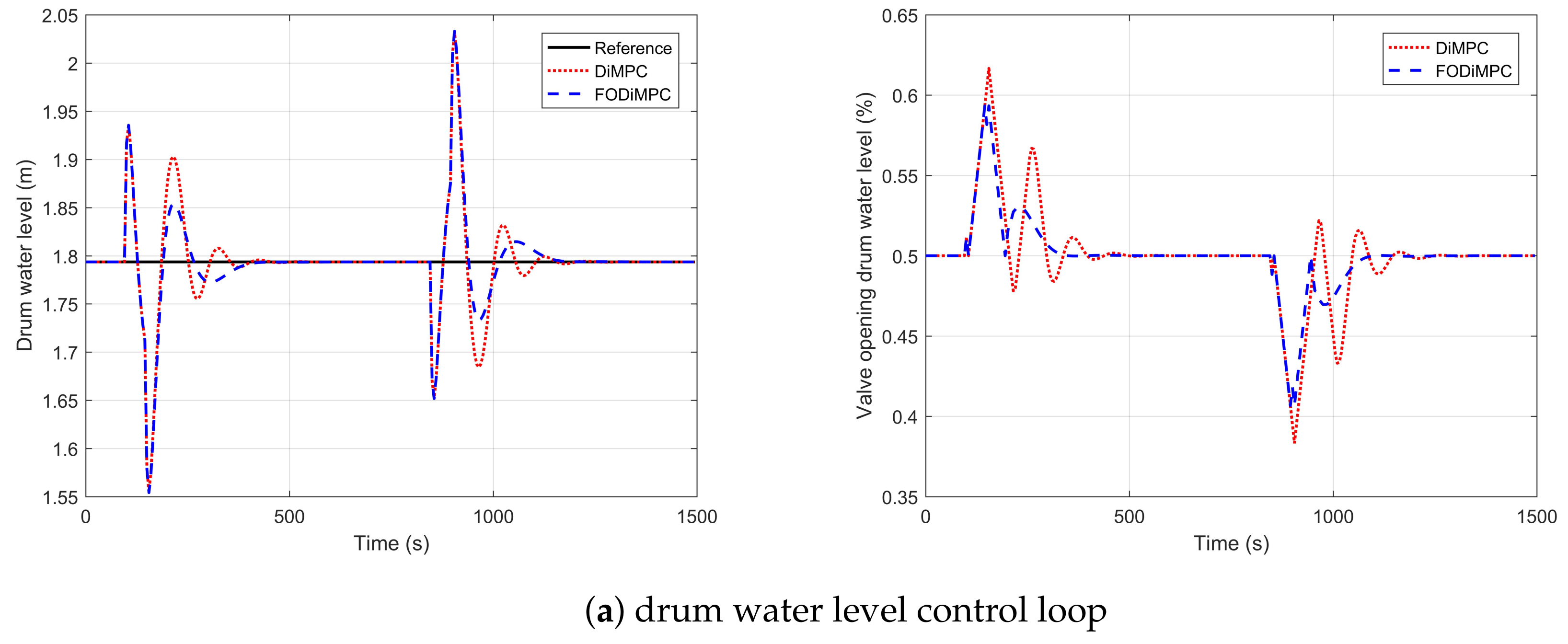
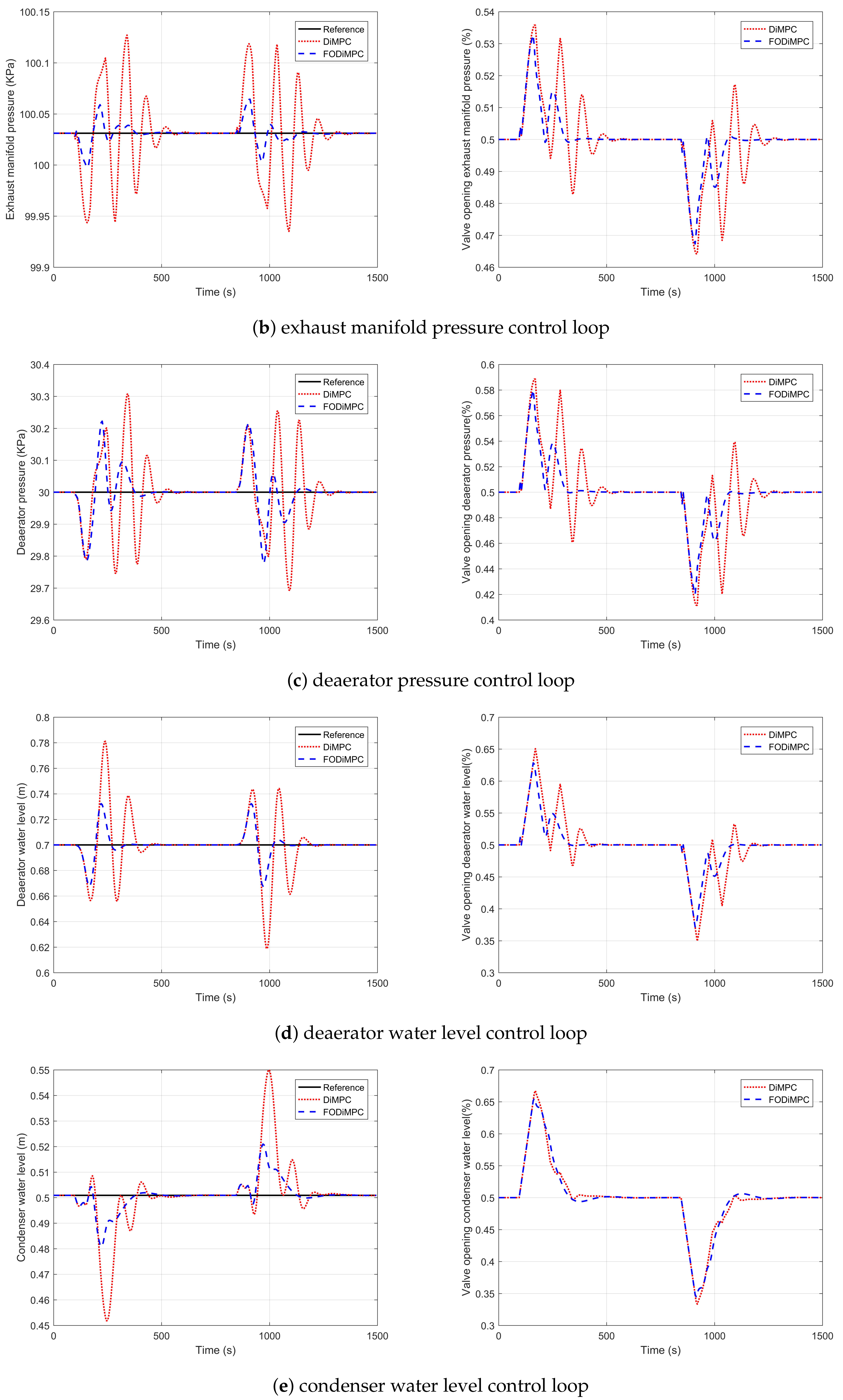
4.2. Reference Tracking Performance

According to the results from previous section, The fractional orders for the five sub-loops are chosen as 6.2, 0.62, 2.2, 1.2 and 1.2, respectively. The following indexes are applied to evaluate the performance of the FOMPC and MPC, including the Integrated Absolute Relative Error ($IARE$), Integral Secondary control output ($ISU$), Ratio of Integrated Absolute Relative Error ($RIARE$), Ratio of Integral Secondary control output ($RISU$) and combined index (J).

$$IAR{E}_i=\sum _{k=0}^{N_s-1}\left|r_i\left(k\right)-y_i\left(k\right)\right|/r_i\left(k\right)(i=1,2,\cdots ,5)$$

(23)

$$IS{U}_i=\sum _{k=0}^{N_s-1}{\left(u_i\left(k\right)-u_{ssi}\left(k\right)\right)}^2(i=1,2,\cdots ,5)$$

(24)

$$RIAR{E}_i(C_2,C_1)=\frac{IAR{E}_i\left(C_2\right)}{IAR{E}_i\left(C_1\right)}(i=1,2,\cdots ,5)$$

(25)

$$RIS{U}_i(C_2,C_1)=\frac{IS{U}_i\left(C_2\right)}{IS{U}_i\left(C_1\right)}(i=1,2,\cdots ,5)$$

(26)

$$J(C_2,C_1)=\frac{1}{5}\sum _{i=1}^5\frac{w_{1}RIAR{E}_i(C_2,C_1)+w_{2}RIS{U}_i(C_2,C_1)}{w_1+w_2}$$

(27)

where $u_{ssi}$ is the steady state value of $i^{th}$ input; $C_1$,$C_2$ are the two compared controllers; the weighting factors $w_1$ and $w_2$ in Equation (27) are chosen as $w_1=w_2=0.5$.

In the Reference tracking experiment, step signals are introduced to the system at different time. The setpoints for the five loops are shown in

Table 4. Setpoints for different loops in the experiments.

Time (s)	2–300	300–600	600–900	900–1200	1200–1500
Drum Water Level (m)	2	2	2	2	2
Exhaust Manifold Pressure(MPa)	100.03	116	116	116	116
Deaerator Pressure (KPa)	30	30	35	35	35
Deaerator Water Level(m)	0.7	0.7	0.7	0.8	0.8
Condenser Water Level(m)	0.5	0.5	0.5	0.5	0.6

.

The simulation results about reference tracking performance are shown in Figure 3. And the performance indexes are shown in

Table 5. Indexes for $IARE$ and $ISU$ in the reference tracking experiment.

Index		Loop 1	Loop 2	Loop 3	loop 4	Loop 5
$IARE$	MPC	1.2614	1.6972	1.9464	2.0500	2.9060
	FOMPC	1.3337	1.6411	1.8813	1.5570	1.9686
$ISU$	MPC	0.0302	0.4776	0.1330	0.1577	1.6925
	FOMPC	0.0205	0.4719	0.1014	0.1371	1.7689

and

Table 6. Indexes for $RIARE$ and $RISU$ in the reference tracking experiment (MPC is the $C_2$ and FOMPC the $C_1$ according to Equations (25) and (26)).

Index	Loop 1	Loop 2	Loop 3	Loop 4	Loop 5
$RIARE$	0.9458	1.0342	1.0346	1.3166	1.4762
$RISU$	1.4729	1.0119	1.3119	1.1503	0.9568

.

The combined index J for the reference tracking case is 1.1711. Both from the Figure 3 and performance indexes, it can be concluded that the FOMPC outperforms the MPC in reference tracking experiment. The response time and overshoot are both smaller in FOMPC than those in the traditional MPC. From Table 5, the $ISU$s for sub-loop 5 are similar, however, the $IARE$s are much different from each other. This is caused by the interaction between water levels of deaerator and condenser water level. The condenser has a smaller volume than the deaerator, hence, the water level in condenser changes a lot along with the deaerator water level.

4.3. Load Disturbance Rejection Performance

In the simulation of the load disturbance rejection experiment, 20% load increase from time period 100 s to 150 s and 20% load decrease from time period $850s$ to $900s$ are introduced in the steam/water loop. And the simulation results for load disturbance rejection experiment are shown in Figure 4 and

Table 7. Indexes for $IARE$ and $ISU$ in the load fluctuation experiment.

Index		Loop 1	Loop 2	Loop 3	Loop 4	Loop 5
$IARE$	MPC	3.5312	0.0686	0.6469	4.8710	3.4694
	FOMPC	3.1523	0.0129	0.3402	1.6632	1.6197
$ISU$	MPC	0.2403	0.0393	0.2379	0.5215	0.7876
	FOMPC	0.1452	0.0206	0.1253	0.3114	0.7855

and

Table 8. Indexes for $RIARE$ and $RISU$ in the load fluctuation experiment (MPC is the $C_2$ and FOMPC the $C_1$ according to Equations (25) and (26)).

Index	Loop 1	Loop 2	Loop 3	Loop 4	Loop 5
$RIARE$	1.1202	5.3201	1.9016	2.9287	2.1420
$RISU$	1.6551	1.9049	1.8988	1.6748	1.0027

.

The combined index J for the load fluctuation case is 2.1549. Compared with MPC, the FOMPC method reduces the tracking error by 168%, and reduces the amount of control effort changes by 62.7%. The FOMPC has a significant improvement than the MPC method. With less control effort, the FOMPC can achieve better load disturbance rejection performance than the MPC.

5. Conclusions

By replacing the integer cost function with a fractional order one, the fractional order MPC based on EPSAC framework is applied to the steam/water loop in large scale ships. The comparison between FOMPC and MPC shows the FOMPC has better performance both in the reference tracking and load disturbance rejection. Different fractional orders are applied to the five sub-loops in steam/water loop, and it is concluded that within a certain range of the fractional order, the larger the order leads to better performance.

References

1. Lamnabhi-Lagarrigue, F.; Annaswamy, A.; Engell, S.; Isaksson, A.; Khargonekar, P.; Murray, R.M.; Nijmeijer, H.; Samad, T.; Tilbury, D.; Van den Hof, P. Systems & Control for the future of humanity, research agenda: Current and future roles, impact and grand challenges. Annu. Rev. Control 2017, 43, 1–64. [Google Scholar]
2. Drbal, L.; Westra, K.; Boston, P. Power Plant Engineering; Springer Science & Business Media: Berlin/Heidelberg, Germany, 2012. [Google Scholar]
3. Zhao, S.; Maxim, A.; Liu, S.; De Keyser, R.; Ionescu, C.M. Distributed model predictive control of steam/water loop in large scale ships. Processes 2019, 7, 442. [Google Scholar] [CrossRef] [Green Version]
4. Romero, M.; Mañoso, C.; Ángel, P.; Vinagre, B.M. Fractional-order generalized predictive control: Formulation and some properties. In Proceedings of the 2010 11th International Conference on Control Automation Robotics & Vision, Singapore, 7–10 December 2010; pp. 1495–1500. [Google Scholar]
5. Samad, T. A survey on industry impact and challenges thereof [technical activities]. IEEE Control Syst. Mag. 2017, 37, 17–18. [Google Scholar]
6. Liu, X.; Cui, J. Economic model predictive control of boiler-turbine system. J. Process Control 2018, 66, 59–67. [Google Scholar] [CrossRef]
7. Zhang, F.; Wu, X.; Shen, J. Extended state observer based fuzzy model predictive control for ultra-supercritical boiler-turbine unit. Appl. Therm. Eng. 2017, 118, 90–100. [Google Scholar] [CrossRef]
8. Ławryńczuk, M. Nonlinear predictive control of a boiler-turbine unit: A state-space approach with successive on-line model linearisation and quadratic optimisation. ISA Trans. 2017, 67, 476–495. [Google Scholar] [CrossRef]
9. Ionescu, C.M.; Copot, D. Hands-on MPC tuning for industrial applications. Bull. Pol. Acad. Sci.-Tech. Sci. 2019, 67, 925–945. [Google Scholar]
10. Maxim, A.; Copot, D.; Copot, C.; Ionescu, C.M. The 5W’s for Control as Part of Industry 4.0: Why, What, Where, Who, and When—A PID and MPC Control Perspective. Inventions 2019, 4, 10. [Google Scholar] [CrossRef] [Green Version]
11. De Keyser, R.; Muresan, C.I.; Ionescu, C.M. An efficient algorithm for low-order direct discrete-time implementation of fractional order transfer functions. ISA Trans. 2018, 74, 229–238. [Google Scholar] [CrossRef]
12. Sabatier, J.; Agrawal, O.P.; Machado, J.T. Advances in Fractional Calculus; Springer: Berlin/Heidelberg, Germany, 2007; Volume 4. [Google Scholar]
13. Podlubny, I. Fractional differential equations. Math. Sci. Eng. 1999, 198, 244–252. [Google Scholar]
14. De Keyser, R.; Muresan, C.I.; Ionescu, C.M. Universal direct tuner for loop control in industry. IEEE Access 2019, 7, 81308–81320. [Google Scholar] [CrossRef]
15. Cajo Diaz, R.A.; Copot, C.; Ionescu, C.M.; De Keyser, R.; Plaza Guingla, D.A. Fractional order PD path-following control of an AR.Drone quadrotor. In Proceedings of the 2018 IEEE 12th International Symposium on Applied Computational Intelligence and Informatics (SACI), Timisoara, Romania, 17–19 May 2018; pp. 291–296. [Google Scholar]
16. Saleem, A.; Soliman, H.; Al-Ratrout, S.; Mesbah, M. Design of a fractional order PID controller with application to an induction motor drive. Turk. J. Electr. Eng. Comput. Sci. 2018, 26, 2768–2778. [Google Scholar] [CrossRef]
17. Mohammadikia, R.; Aliasghary, M. A fractional order fuzzy PID for load frequency control of four-area interconnected power system using biogeography-based optimization. Int. Trans. Electr. Energy Syst. 2019, 29, e2735. [Google Scholar] [CrossRef]
18. Cajo, R.; Muresan, C.I.; Ionescu, C.M.; De Keyser, R.; Plaza, D. Multivariable fractional order PI autotuning method for heterogeneous dynamic systems. IFAC-PapersOnLine 2018, 51, 865–870. [Google Scholar] [CrossRef]
19. Zeng, G.Q.; Chen, J.; Dai, Y.X.; Li, L.M.; Zheng, C.W.; Chen, M.R. Design of fractional order PID controller for automatic regulator voltage system based on multi-objective extremal optimization. Neurocomputing 2015, 160, 173–184. [Google Scholar] [CrossRef]
20. Cajo Diaz, R.A.; Mac Thi, T.; Copot, C.; Plaza Guingla, D.A.; De Keyser, R.; Ionescu, C.M. Multiple UAVs formation for emergency equipment and medicines delivery based on optimal fractional order controllers. In Proceedings of the Preprints of the 2019 IEEE International Conference on Systems, Man and Cybernetics (SMC), Bari, Italy, 6–9 October 2019; pp. 328–333. [Google Scholar]
21. Cajo, R.; Mac, T.T.; Plaza, D.; Copot, C.; De Keyser, R.; Ionescu, C. A survey on fractional order control techniques for unmanned aerial and ground vehicles. IEEE Access 2019, 7, 66864–66878. [Google Scholar] [CrossRef]
22. Muresan, C.; Birs, I.R.; Folea, S.; Ionescu, C.M. Fractional order based velocity control system for a nanorobot in non-Newtonian fluids. Bull. Pol. Acad. Sci.-Tech. Sci. 2018, 66. [Google Scholar] [CrossRef]
23. Zhang, R.; Zou, Q.; Cao, Z.; Gao, F. Design of fractional order modeling based extended non-minimal state space MPC for temperature in an industrial electric heating furnace. J. Process Control 2017, 56, 13–22. [Google Scholar] [CrossRef]
24. Chen, M.R.; Zeng, G.Q.; Dai, Y.X.; Lu, K.D.; Bi, D.Q. Fractional-Order model predictive frequency control of an islanded microgrid. Energies 2019, 12, 84. [Google Scholar] [CrossRef] [Green Version]
25. Zhao, S.; Maxim, A.; Liu, S.; De Keyser, R.; Ionescu, C. Effect of control horizon in model predictive control for steam/water loop in large-scale ships. Processes 2018, 6, 265. [Google Scholar] [CrossRef] [Green Version]
26. De Keyser, R. Model based predictive control for linear systems. In UNESCO Encyclopaedia of Life Support Systems, Robotics and Automation, Vol XI, Article Contribution 6.43.16.1; Eolss Publishers Co Ltd.: Oxford, UK, 2003. [Google Scholar]
27. Romero, M.; de Madrid, A.P.; Vinagre, B.M. Arbitrary real-order cost functions for signals and systems. Signal Process. 2011, 91, 372–378. [Google Scholar] [CrossRef]
Figure 1. Structure of the steam/water loop [25] (reproduced with permission from Zhao, S.; Maxim, A.; Liu, S.; De Keyser, R.; and Ionescu, C, Processes; published by MDPI, 2018.).
Processes 08 00451 g001
Figure 2. Outputs with different fractional orders for the five sub-loops.
Processes 08 00451 g002
Figure 3. Outputs of the steam/water loop with FOMPC and MPC in the reference tracking experiment (The outputs are listed on the left hand, and the inputs are listed on the right hand).
Processes 08 00451 g003aProcesses 08 00451 g003b
Figure 4. Outputs variables with FOMPC and MPC in the load fluctuation experiment (The outputs are listed on the left hand, and the inputs are listed on the right hand).
Processes 08 00451 g004aProcesses 08 00451 g004b