Semi-Supervised Ensemble Classification Method Based on Near Neighbor and Its Application

Abstract

Semi-supervised learning can be used to solve the problem of insufficient labeled samples in the process industry. However, in an actual scenario, traditional semi-supervised learning methods usually do not achieve satisfactory performance when the small number of labeled samples is subjective and inaccurate and some do not consider how to develop a strategy to expand the training set. In this paper, a new algorithm is proposed to alleviate the above two problems, and consequently, the information contained in unlabeled samples can be fully mined. First, the multivariate adaptive regression splines (MARS) and adaptive boosting (Adaboost) algorithms are adopted for co-training to make the most of the deep connection between samples and features. In addition, the strategies, pseudo-labeled dataset selection algorithm based on near neighbor degree (DSSA) and pseudo-labeled sample detection algorithm based on near neighbor degree selection (SPDA) are adopted to enlarge the dataset of labeled samples. When we select the samples from the pseudo-labeled data to join the training set, the confidence degree and the spatial relationship with labeled samples are considered, which are able to improve classifier accuracy. The results of tests on multiple University of California Irvine (UCI) datasets and an actual dataset in the aluminum electrolysis industry demonstrate the effectiveness of the proposed algorithm.

1. Introduction

Mechanisms and data-driven models are playing more and more important roles in the field of engineering [1]. Traditional machine learning algorithms can only be trained by labeled datasets [2]. A lot of manpower and material resources are consumed when experts mark unlabeled samples, but unlabeled data is easily obtained in the production equipment. In addition, in some cases, manually labeled samples have a small number of errors, which affects the subsequent training. For traditional supervised learning methods, the use of only a few labeled samples results in a loss of information, because the information in unlabeled samples cannot be completely extracted [3,4,5], and the accuracy of the trained classifiers is not ideal. The semi-supervised learning method directly affects the effectiveness of machine learning technology for practical tasks, because this method uses only a small number of labeled samples and makes full use of a large number of pseudo-labeled samples to improve the performance of the classifiers. In recent years, it has gradually become a study hotspot for research on current mainstream technology of unlabeled samples [6].

Semi-supervised learning is an important research method in data mining and machine learning because it makes full use of limited labeled samples and select unlabeled samples to train the model. According to different learning tasks, semi-supervised learning is mainly divided into semi-supervised clustering methods and semi-supervised classification methods [7]. Both methods improve the learning performance of limited labeled samples. The current semi-supervised learning methods can be roughly divided into the following four categories: generative model-based methods, semi-supervised SVM methods, graph-based methods, and disagreement-based methods [8]. The method based on generative models originates from the assumption that all data (whether labeled or not) are generated by the same underlying model, such as the model by Shahshahani who assumed that the original sample satisfies the Gaussian distribution, and then used the maximum likelihood probability to fit a Gaussian distribution which is usually called the Gaussian mixture model (GMM) [9], but the result of this method depended too much on the choice of model. As it turns out, the model assumptions must be accurate, and the hypothesized generative model must match the real data distribution. Semi-supervised support vector machine (SVM) is a generalization of the support vector machine for semi-supervised learning [10]. The interval of the SVM on all training data (including labeled and unlabeled data) is adjusted to the maximum by determining the hyperplane and the label assignment for unlabeled data. Joachims proposed the TSVM (transductive SVM) method for binary classification problems which took specific test sets into account and tried to minimize the misclassification of these specific examples. This method has a large number of applications in terms of text classification and achieves very good effect [11]. The graph-based method maps all labeled and unlabeled datasets into a graph, and each sample in the datasets corresponds to a node on the graph. Sample labels are propagated from labeled to unlabeled samples with a certain probability, and the performance of this method also depends too much on the construction method of the data graph [12].

Learning the same dataset from multiple different perspectives, disagreement-based semi-supervised learning focuses on the "divergence" between multiple learners which also predicts unlabeled samples through the trained classifiers to achieve the purpose of expanding the training set. This type of technology is less affected by model assumptions, non-convexity of loss functions, and issues of data size. The theoretical foundation of the learning method is relatively well established and, it is so simple and effective that the applicable scope of this method is more extensive [7].

The co-training process is a form of semi-supervised learning based on disagreement, which requires that the data have two fully redundant views that satisfy the conditional independence [13]. The general process of standard co-training, as a typical representative of disagreement-based semi-supervised learning, is as follows: (1) Use labeled data to train a classifier on each view, (2) each classifier labels unlabeled samples and selects a certain number of labels with the highest confidence and the samples are added to the training set; (3) each classifier updates the model with the new samples; and (4) repeats steps two and three until, for each classifier, the number of iterations reaches the preset value or the classifier does not change [14]. Usually, it is required that the data information is sufficient and redundant, and the conditions for finding two independent and complementary views are too harsh. It is difficult to ensure that the two models have different views, let alone different and complementary information. Researchers have found that complementary classifications sub-models can be used to relax the requirement [15]. Even if the same dataset is used, the resulting prediction distributions are different, and therefore the classifiers can be enhanced according to the method of co-training [16].

Abdelgayed proposed a semi-supervised machine learning method based on co-training to solve fault classification in transmission and distribution systems of microgrids [17]. Yu proposed a multi-classifier integrated progressive semi-supervised learning method, using different classifiers obtained by random subspace technology and expanded the training set through a progressive training set generation process [18]. Liu used a random forest algorithm for semi-supervised learning to select pseudo-labeled samples from unlabeled samples and considered the label confidence of the unlabeled samples and the positional relationship with the edge of the classification surface to improve the classification performance [19]. Zhang used regression prediction results to integrate and solve the problem encountered in image processing of separating the foreground from the background of the image [20].

While semi-supervised learning methods have been successfully applied in a variety of scenarios, the randomness of the selection of unlabeled samples during the training process has resulted in unstable and less robust results [21]. The use of ensemble learning can alleviate this problem caused by the selection of unlabeled samples by unifying the results of different learning methods. Using semi-supervised ensemble learning methods to obtain more stable classification results is essential for industry [22,23]. At the same time, however, the use of semi-supervised ensemble learning methods has the following limitations when applied in industry:

1. A large amount of data collected in the industry is mainly labeled by workers through subjective and uncertain empirical knowledge [24]. The impact of the training result due to wrongly labeled samples is huge when the total number of training sets is not large enough;

2. Most semi-supervised ensemble learning methods do not consider how to develop a strategy to select useful samples and eliminate redundant samples in order to expand the training set.

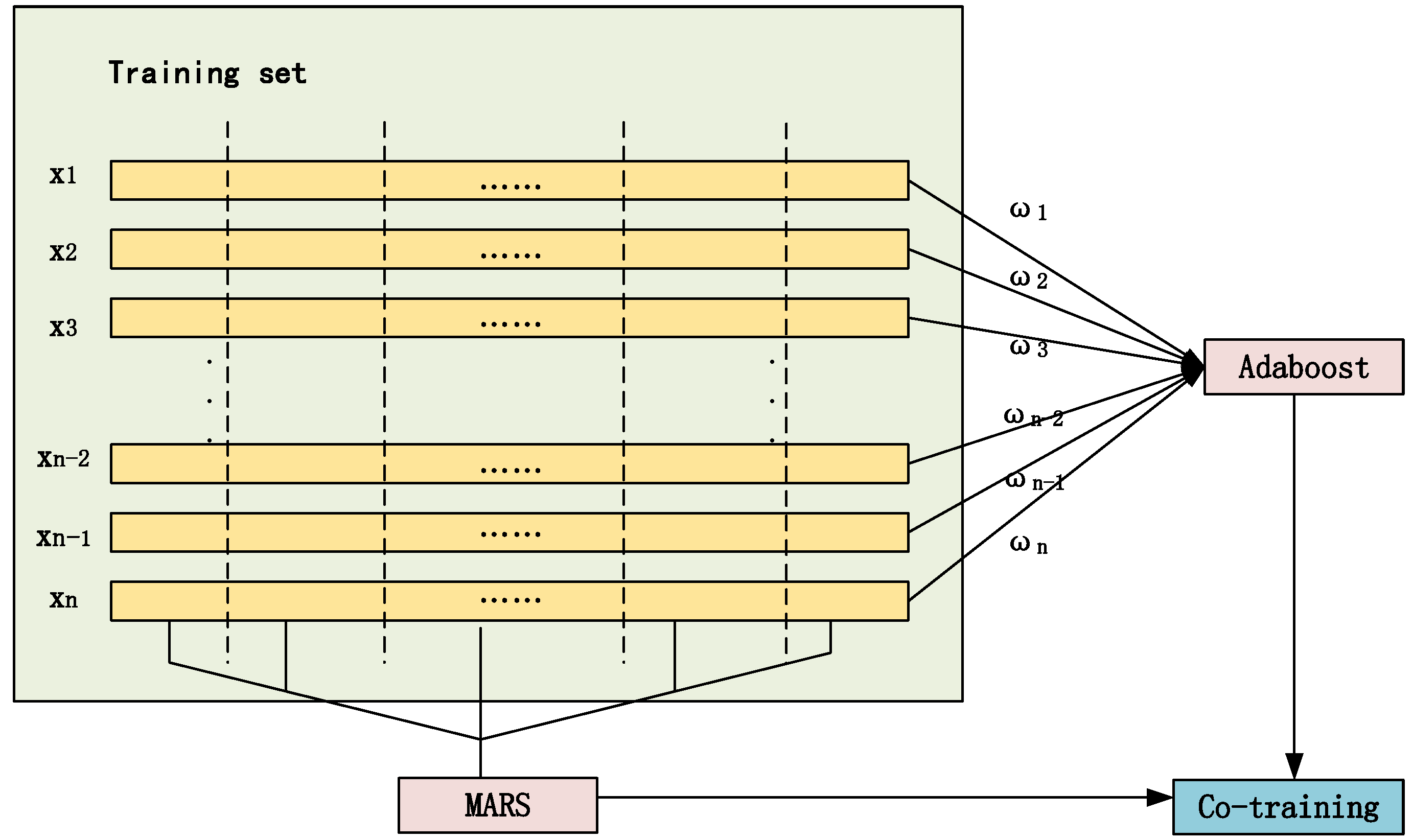
In order to solve the limitations of traditional semi-supervised ensemble learning methods, a semi-supervised neighbor ensemble learning method (SSNEL) based on the multivariate adaptive regression splines (MARS) and adakptive boosting (Adaboost) algorithms as sub-models is proposed in this paper. This method performs co-training based on the "complementarity" formed by the significant difference in the weighting rules of the MARS and Adaboost algorithms during the training process. On the one hand, the MARS algorithm pays attention to the influence of each feature on the classification results and the relationship between the features during the training process, and ignores the role of different samples on the ability of the classifier [25]. On the other hand, the Adaboost algorithm is concerned with only the different roles of the samples, but ignores the differences of each feature and the connections between the features [26]. Theoretically, using two strong subclassifiers, the co-training, based on the MARS and Adaboost algorithms, to a certain extent, reduces the harm caused by the wrongly labeled samples to the generalization ability of the model. In addition, it improves the robustness and prevents "convergence" between homogeneous classifiers during continuous training [27]. After each time using the subclassifiers to obtain the pseudo-labeled samples, in order to find the wrong samples and the samples that do not significantly improve the generalization ability of the model, a series of redundant sample removal algorithms based on the near neighbor degree model are established. Therefore, the SSNEL finds the optimal pseudo-labeled samples to expand the training set and ensures that the best classification results are obtained after retraining with the training set after the addition of new pseudo-labeled samples. The experiment used multiple different real datasets from the University of California Irvine machine learning knowledge base for verification. The results reflect that the SSNEL performs better than traditional semi-supervised ensemble learning methods in most real datasets, and it is outstanding for industrial applications of aluminum electrolytic superheat state classification.

The MARS algorithm builds models of the form:

$$\widehat{f}\left(x\right)={\displaystyle \sum _{i=1}^k{{\displaystyle c}}_i{{\displaystyle B}}_i\left(x\right)}$$

(1)

The model is the weighted sum of basis function values. Each ${{\displaystyle c}}_i$ is a constant coefficient, and each ${{\displaystyle B}}_i\left(x\right)$ can be one of the following three forms: (1) a constant; (2) a hinge function which has the form $\max (0,\mathrm{x}-\mathrm{constant})$ or $\max (0,\mathrm{constant}-x)$, the MARS algorithm automatically selects variables and values of those variables for knots of the hinge functions; and (3) a product of two or more hinge functions. These basis functions can model interaction between two or more variables. The MARS algorithm builds a model in two phases, i.e., the forward and the backward pass. This two-stage approach is the same as that used by recursive partitioning trees [28].

The Adaboost algorithm first obtains a weak classifier by learning from a training sample set. Subsequently, in every retraining a new training sample set is formed by the misclassified samples and supplementary samples, and thus the ability of the classification of a weak classifier is improved [29]. The classification of certain data is determined by the weight of each classifier and samples, but the links between different attributes are not taken into account during classification. Inspired by redundant view conditions for co-training, theoretically, the strong complementarity between the two algorithms can make them better in co-training.

This paper is divided into six chapters, and the main content of each chapter is summarized as follows: Section 1 is an introduction, which describes the research background and core issues of this method; Section 2 presents the components and design of semi-supervised neighbor ensemble learning; Section 3 details the algorithm implementation and how to select useful pseudo-labeled samples; the validation work is in Section 4 which includes the comparison of this method with its competitors on the University of California Irvine (UCI) datasets; Section 5 presents the application and mechanism verification of this method on the aluminum electrolytic industry dataset; and the conclusions and contributions of this study are in Section 6.

2. Semi-Supervised Neighbor Ensemble Learning

Figure 1 provides an overview of the SSNEL. On the one hand, the MARS algorithm ignores the differences of different samples; on the other hand, the Adaboost algorithm is a representative boosting algorithm, which uses the strategy of adjusting the weights of samples according to the classification results of the basic classifiers to obtain better classification results. However, at the same time it does not take advantage of more information that the correlations and differences of different attributes contain. When the number of labeled samples is small or the manual labeling has some errors, the traditional classification results are inaccurate. From the point of view of co-training, as is shown in Figure 2, the MARS and Adaboost algorithms, as the base classifiers, have a certain degree of "complementarity". Both methods are used to introduce unlabeled samples to integrate semi-supervised training which improves the classification ability of both and improves the robustness. That is to say, the method greatly reduces the impact of misclassified samples and mislabeled samples on each iteration in traditional co-training. The commonly used co-training methods often use basic classifiers such as k-nearest neighbor and decision tree, but the performance of the basic classifiers is not good enough to deal with inaccurate labeled samples or when the size of the labeled sample set at the industrial site is not large enough [30]. The misclassified samples that are obtained have a greater impact on the subsequent training, and as a result the generalization ability of the final classifier is not increased. From this perspective, the use of more powerful classification improvement methods brings more useful information to the iterative process. Therefore, a semi-supervised ensemble learning algorithm using the MARS and Adaboost algorithms is proposed.

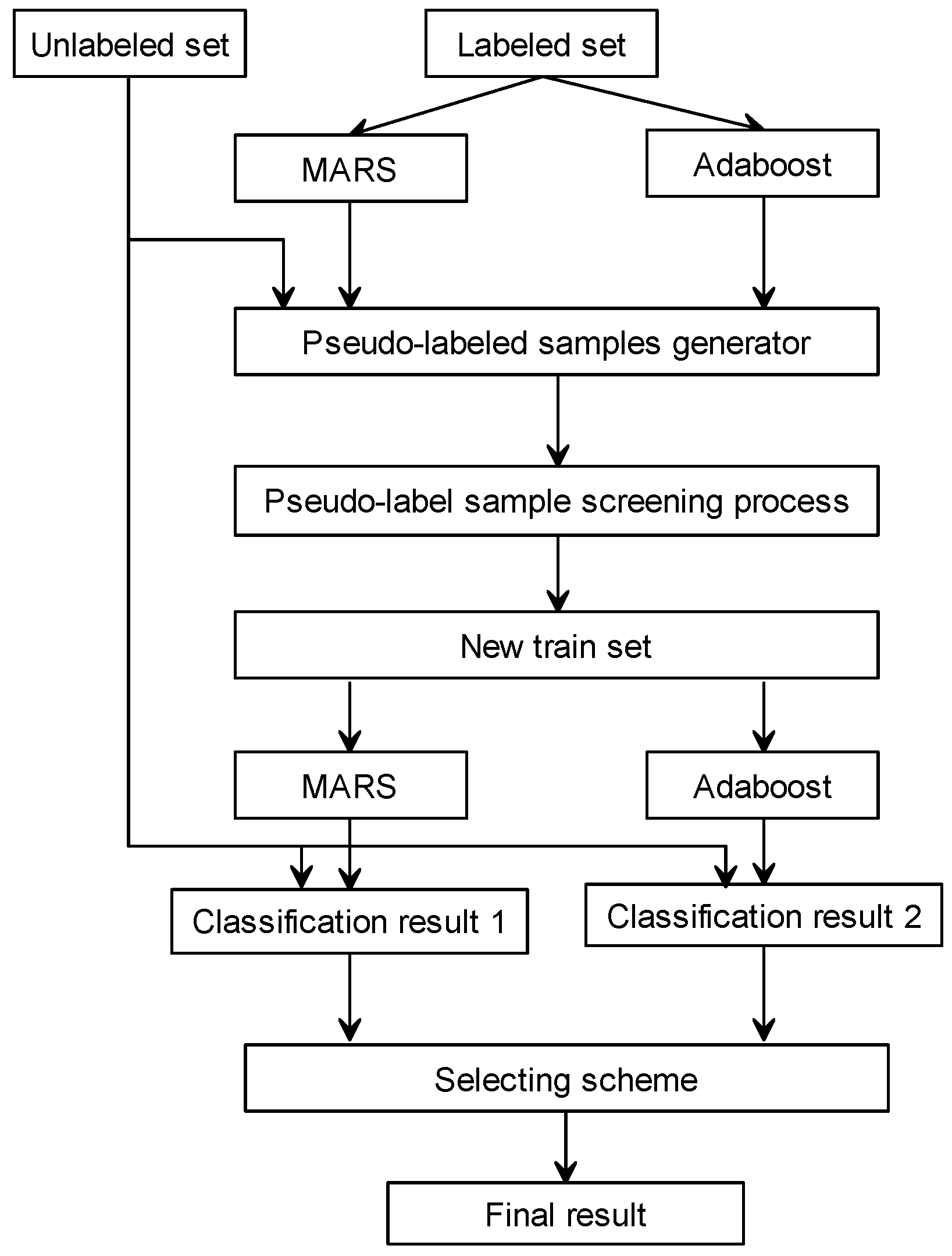
3. Algorithm Implementation

Algorithm 1 is an implementation step of the SSNEL. For all the data obtained, first, divide all data samples into a labeled sample set $T_l$ containing $l$ groups of samples and an unlabeled sample set $T_u$ containing $u$ groups of samples. $T_l=\left\{\left(x_1,y_1\right),\left(x_2,y_2\right),\dots ,\left(x_l,y_l\right)\right\}$, $x_i\left(i\in \left\{1,\dots l\right\}\right)$ indicates labeled samples ($y_i$ denotes the label of corresponding sample $x_i$) and $T_u=\left\{x_{l+1},x_{l+2},\dots ,x_{l+u}\right\}$, $x_i\left(i\in \left\{l+1,\dots l+u\right\}\right)$ is unlabeled samples. Then, use the labeled sample set to initialize the multivariate adaptive regression spline and Adaboost classifiers. The two obtained classifiers are expressed as $F_m$ and $F_a$. In the first iteration, given a subset of unlabeled sample set $U=\left\{u_1,u_2,\dots ,u_s\right\}$, the samples can be predicted by $F_m$ and $F_a$. Next, a pseudo-labeled dataset selection algorithm based on near neighbor degree (DSSA) is applied to pick a useful result from the results obtained by $F_m$ and $F_a$.

Algorithm 1. SSNEL

Require: Input: the labeled training set $T_l$; the selected unlabeled sample set $U$; the number of samples of subset in every iteration $s$; the classifier set contains MARS and Adaboost $F=\left\{F_m,F_a\right\}$.

Ensure: 1: Initialize the current classifier $F_m$ and $F_a$ using $T_l$; 2: While$\left|T_u\right|\ge s$: 3: Select subset $U=\left\{u_1,u_2,\cdots ,u_s\right\}$ from $T_u$; 4: Obtain two pseudo-labeled sample set according to the classification results of $U$ with $F_m$ and $F_a$; 5: Call the pseudo-labeled dataset selection algorithm based on near neighbor degree (DSSA) in Algorithm 2 to generate a more reliable pseudo-labeled sample set $U$; 6: For the pseudo-labeled sample set, call the pseudo-labeled sample detection algorithm based on near neighbor degree (SPDA) in Algorithm 3 to find useful sample set $R$; 7: Update the training set $T_l$ and unlabeled dataset $T_u$; 8: Until the unlabeled samples is run out;

Output: Final training set including labeled samples and useful pseudo-labeled samples

For a single classifier, the predicted labels can be denoted by $Y_u=\left\{y_1,y_2,\dots ,y_s\right\}$, and the pseudo-labeled sample set are denoted by $T_p$. Retrain MARS and Adaboost classifiers with corresponding $T_l\cup T_p$, and the result predicted by the classifier is $Y_u^{\prime }$, the near neighbor degree of $Y_u$ and $Y_u^{\prime }$ is expressed as follows:

$$\Delta 1=\frac{Y_u·Y_u^{\prime }{}^T}{{\Vert Y_u\Vert }^2\times {\Vert Y_u^{\prime }\Vert }^2}$$

(2)

The near degree between selected subset and the labeled sample set in this iteration is also considered as follows:

$$\Delta 2=\frac{{\displaystyle {\sum }_{c=1}^C\left(P_c-\overline{P}\right)\left(L_c-\overline{L}\right)}}{\sqrt{{{\displaystyle {\sum }_{c=1}^C\Vert P_c-\overline{P}\Vert }}^2}\sqrt{{{\displaystyle {\sum }_{c=1}^C\Vert L_c-\overline{L}\Vert }}^2}}$$

(3)

$$\overline{P}=\frac{{\displaystyle {\sum }_{c=1}^C{P}_c}}{C}$$

(4)

$$\overline{L}=\frac{{\displaystyle {\sum }_{c=1}^C{L}_c}}{C}$$

(5)

$$P_c=\frac{1}{{\displaystyle {\sum }_{i=1}^{s}1\left\{y_i=c\right\}}}{\displaystyle \sum _{\forall x_i\in T_p}{x}_i\cdot 1\left\{y_i=c\right\}}$$

(6)

$$L_c=\frac{1}{{\displaystyle {\sum }_{i=1}^{l}1\left\{y_i=c\right\}}}{\displaystyle \sum _{\forall x_i\in T_l}{x}_i\cdot 1\left\{y_i=c\right\}}$$

(7)

where $C$ is the number of categories in the dataset and $s$ is the number of samples in the selected subset $U$.

On the one hand, it is obvious that $\Delta 1$ reflects the effect of introducing pseudo-labeled samples to the training set on the classification. The larger $\Delta 1$ is, the more reliable the result. On the other hand, $\Delta 2$ reflects the near neighbor degree of pseudo-labeled samples and training set samples in the same category. When the value of $\Delta 2$ is too small, it means that the distribution of the samples classified into the same class is significantly different from the training set. However, a value that is too large $\Delta 2$ means that the pseudo-labeled samples bring little improvement in classification ability and even reduce the stability of classifiers.

Then, we obtain:

$$\Delta =\Delta 1+\eta \cdot \Delta 2$$

(8)

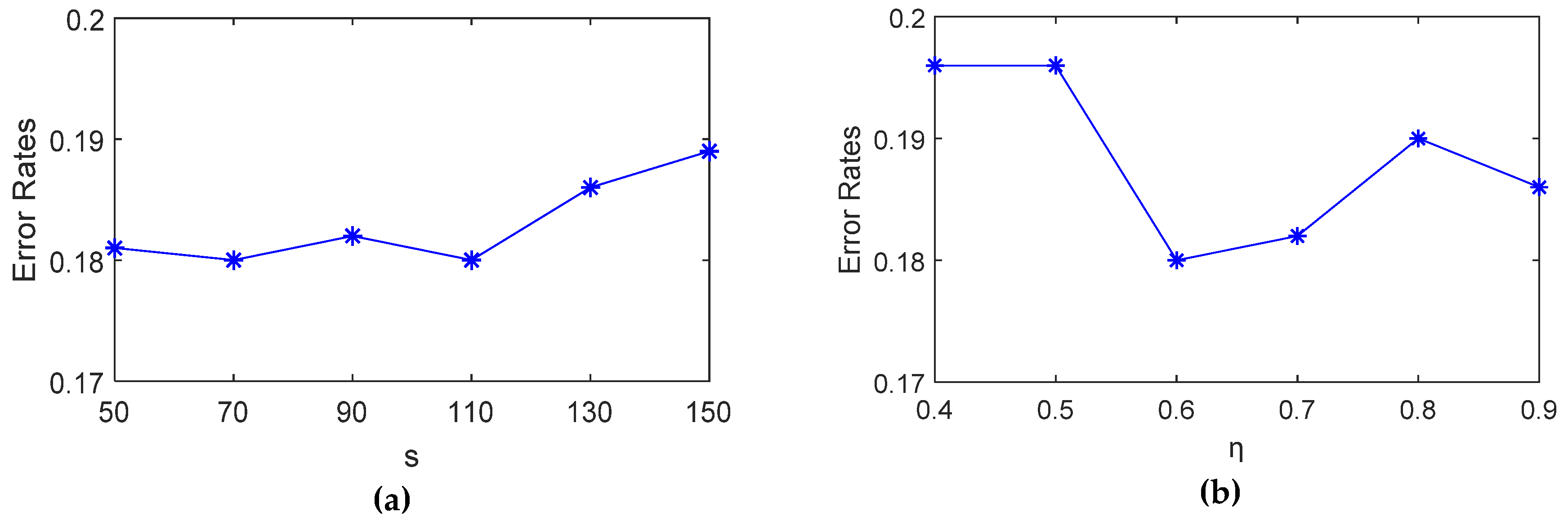
where $\eta$ is a preset parameter, and in the two pseudo-labeled sample sets obtained by the MARS and Adaboost classifiers, select the one which has a larger $\Delta$. The pseudo code of DSSA is Algorithm 2.

Algorithm 2. DSSA

Require: Input: the labeled training set $T_l$; the selected unlabeled sample subset $U$; the classifier set contains MARS and Adaboost $F=\left\{F_m,F_a\right\}$.

Ensure: 1: For a single classifier, generate the classification results $Y_u$ of set $U$ and get a group of pseudo-labeled samples; 2: Retrain MARS and Adaboost with corresponding $T_l\cup T_p$, and the results predicted by the classifiers is $Y_u^{\prime }$ 3: Calculate the neighbor degree $\Delta 1$ of $Y_u$ and $Y_u^{\text{'}}$ 4: Compare the samples in dataset $U$ and $T_l$ to calculate the near neighbor degree $\Delta 2$; 5: Calculate the final near neighbor degree $\Delta =\Delta 1+\eta \cdot \Delta 2$; 6: In the two pseudo-labeled sample sets obtained by MARS and Adaboost, select the one which has a larger $\Delta$.

Output: A more reliable pseudo-labeled sample set.

However, not all the samples in the selected pseudo-labeled dataset are useful for classification. Fortunately, the pseudo-labeled sample detection algorithm based on near neighbor degree (SPDA) is a useful approach to test the validity of a sample. The selected pseudo-labeled dataset is denoted by $U=\left\{u_1,u_2,\dots ,u_s\right\}$, and the training sample subset in the training set corresponding to the category of $u_1$ is $K_i=\left\{k_{i1},k_{i2},\dots ,k_{ik}\right\}$. The outlier factor of the pseudo-labeled sample can be calculated by:

$$N_i={\displaystyle \sum _{q=1}^{k}f\left(\xi \left(u_i,C_q\right),\overline{{\xi }_i}\right)}$$

(9)

$$\xi \left(x_i,x_j\right)=\sqrt{{\displaystyle \sum _{m=1}^M\left[r_m{\left(x_{im}-x_{jm}\right)}^2\right]}}$$

(10)

$$\overline{{\xi }_i}=\frac{{\displaystyle {\sum }_{j=1}^k\xi \left(u_i,C_j\right)}}{k}$$

(11)

$$f\left(\xi \left(U_i,C_q\right),\overline{{\xi }_i}\right)=\{\begin{array}{c}0,\xi \left(U_i,C_q\right)\ge \overline{{\xi }_i}\\ 1,\xi \left(U_i,C_q\right)<\overline{{\xi }_i}\end{array}$$

(12)

where $\xi \left(x_i,x_j\right)$ is the near neighbor degree between sample $x_i$ and sample $x_j$, and $M$ represents the number of attributes, $r_m$ represents the weight of the effect of the feature on the classification result.

For every unlabeled sample, count the number of samples whose near neighbor degree is greater than the mean, and get the outlier factor vector $N=\left[N_1,N_2,\dots ,N_u\right]$. And the sign vector $G=\left\{g_1,g_2,\dots ,g_s\right\}$ for the selected pseudo-labeled dataset $U$ (where $s$ is the number of samples in $U$). And $g_i$ is defined as follows:

$$g_i=\{\begin{array}{cc}0,& N_i\ge \overline{N}\\ 1,& N_i\le \overline{N}\end{array}$$

(13)

$$\overline{N}=\frac{1}{s}{\displaystyle \sum _{i=1}^s{N}_i}$$

(14)

The new training set $T_l$ is augmented as follows:

$$T_l=T_l\cup R$$

(15)

And the unlabeled dataset is:

$$T_u=T_u-U$$

(16)

where $R$ means the set of retained pseudo-labeled dataset.

Finally retrain the subclassifiers with the new training set in the next iteration until all unlabeled samples are used up.

Algorithm 3. SPDA

Require: Input: the labeled training set $T_l$; the selected unlabeled sample subset $U$; the more reliable pseudo-labeled sample set selected in DSSA including $U$ and $Y_u$.

Ensure: 1: Divide current training set $T_l$ into $c$ groups according to the types of pseudo-tags(c is the number of categories included in the sample set); 2: For each $U_i\in U$: 3: Calculate the near neighbor degree of $U_i$ and the training set samples in the corresponding category; 4: According to the result of 3, compute the outlier factor $N_i$ of $U_i$; 5: Get the outlier factor vector $N$ and sign vector $G$, screen out sample set $R$ that is beneficial to the improvement of classification ability

Output: the sample set $R$.

4. Algorithm Verification

4.1. Verification on Public Datasets

In order to verify the classification performance of the SSNEL, the experiment was tested on multiple UCI datasets. To estimate the promotion of the performance of subclassifiers, error_rate is used as evaluation indicators [31].

$$error\_rate=\frac{1}{\left|T_e\right|}{\displaystyle \sum _{x_i\in T_e}1\left\{y_i^{*}\ne y_i^{true}\right\}}$$

(17)

where $T_e$ denotes the testing set.

The k-fold cross validation, as a commonly used approach in the field of machine learning, is adopted to get the final results of the SSNEL and other compared methods. The information of the datasets used is shown in

Table 1. Information of the UCI public dataset.

Dataset	Wine	Glass	Yeast	German
Total number of samples	178	214	1484	1000
Total number of attributes	13	10	8	25
Total number of categories	2	7	2	2

. The labeled samples and unlabeled samples are randomly divided in every experience. The proportion of labeled samples in the total sample set is 25%, and the rest are unlabeled samples. The performance of the SSNEL and its competitors on these public datasets are demonstrated, as shown in Figure 3.

When the rate of unlabeled data and labeled data in the UCI dataset is adjusted to 1, 2, 3, and 4 the error rates of SSNEL and its competitors in the classification of each dataset are shown in Figure 3, Figure 4, Figure 5 and Figure 6.

Figure 4, Figure 5, Figure 6 and Figure 7 show that the SSNEL proposed in this paper performs better than its competitors on different datasets. The average error_rate is 0.0925 lower than that obtained by supervised learning algorithms (MARS and Adaboost algorithms) when the rate of unlabeled samples and labeled samples is 3. Compared with traditional co-training, the value is 0.0575 lower. The possible reason could be that the SSNEL reflects the correlation between samples and the interaction between different attributes in a high-dimensional dataset, and the adoption of DSSA and SPDA find the reliable pseudo-labeled sample set and remove the redundant pseudo-labeled samples. To sum up, the SSNEL can improve the ability of classification when it deals with multiple real-life datasets.

4.2. Adjustment of the Parameters

Table 2. Adjustment of the parameters.

Parameters	Default Values	Range
$s$	110	50, 70, 90, 110, 130, 150
$\eta$	0.6	0.4, 0.5, 0.6, 0.7, 0.8, 0.9

lists the default values of the influential parameters. Take the experiment on dataset German as an example. To study a parameter, we adjust the value within a suitable range and set the other parameters to the default value.

Figure 8a,b presents the results of adjustment of parameters. As the number of subset $U$ increases, we find that when $s=110$, the ability of classification is strongest. If $s$ is too large, the final selected pseudo-labeled dataset contains many redundant inaccurate samples that could reduce generalization ability. However, a value of $s$ that is too small could lead to overfitting and the time to train classifiers is longer. On the other hand, when $\eta =0.6$, the ability of classification is strongest. The larger $\eta$ means the distribution of selected pseudo-labeled samples is more similar to the training set. When $\eta$ is too small, the confidence degree of the new training set is not enough to improve the classifier. But if $\eta$ is too large, pseudo-labeled samples do not influent the distribution of training set and even reduce the classification ability.

5. Application on Aluminum Electrolyzer Condition Dataset

The stable running state of the aluminum electrolytic cell can ensure that the aluminum electrolytic cell has a good shape of the bore and improve the current efficiency [32]. 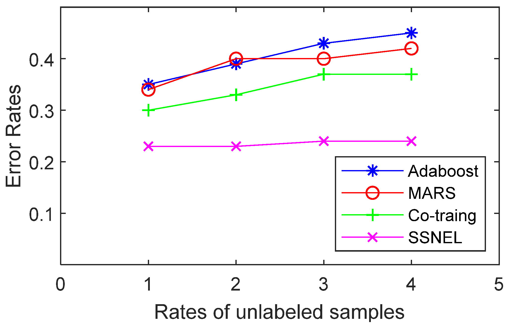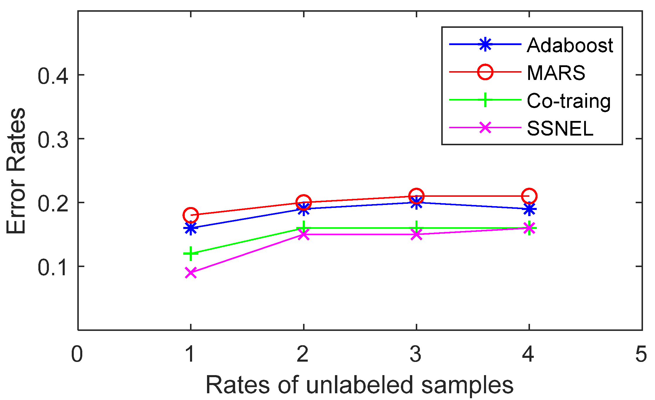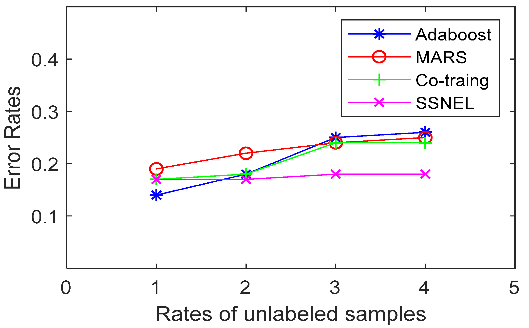By analyzing the relationship between the key process indicators and the state of the electrolyzer condition, 10 process indicators are selected in this experiment as the input of the prediction model, which are needle vibration, swing, effect peak pressure, effect number, aluminum level, electrolyte level, number of overfeeds, number of underfeeds, molecular ratio, and temperature [33]. The judgment results include over stability index (H), moderate stability index (F), and low stability index (L). Experienced workers can add labels to a small number of data samples to judge the current status. In this paper, 2000 samples from a factory in Shandong Province are adopted to validate the applicability of the SSNEL in the field of engineering. We performed ten classification experiments on the same dataset for each algorithm. Because the selection process of the initial training set with labels and unlabeled samples is random, for an algorithm, different sample selections bring some fluctuations.

Table 3. The results of the tests on the aluminum electrolytic cell condition dataset.

Algorithms	Adaboost	MARS	Co-Training	M-Co-Forest	SSNEL
Error_rate	0.273 ± 0.067	0.217 ± 0.153	0.208 ± 0.032	0.198 ± 0.012	0.186 ± 0.004

shows the comparison of the results of this method and its competitors on the aluminum electrolytic cell condition dataset. The results contain the average error_rates and the fluctuation ranges of every algorithm in ten experiments.

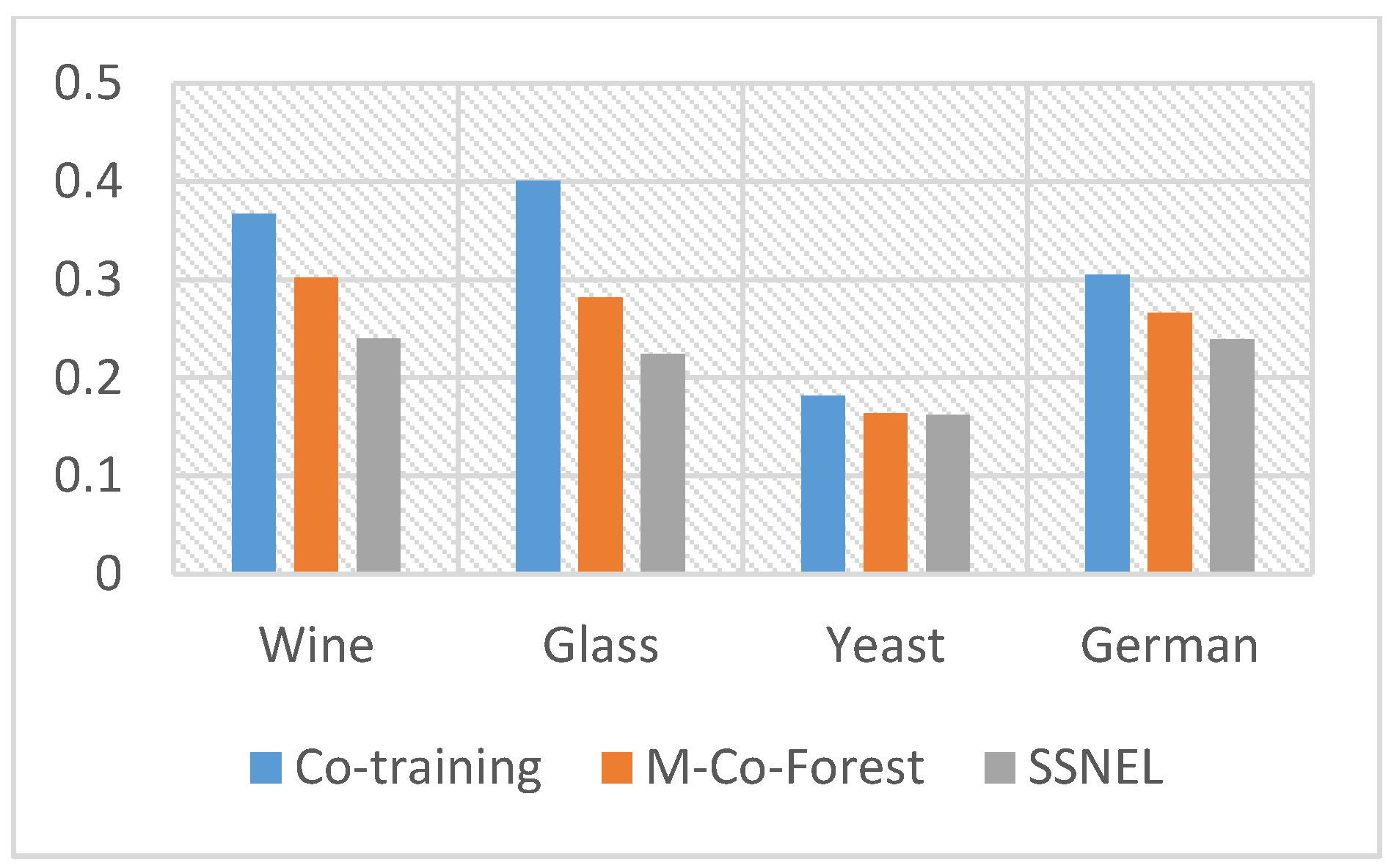
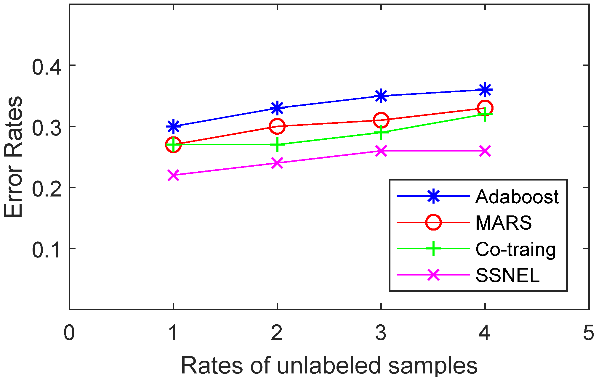
The comparison shows that when a supervised learning algorithm is used to deal with the problem of lacking labeled samples, the classification effect is not satisfactory and the classification of the error rate is greatly affected by the training set. When we use traditional semi-supervised learning algorithms such as co-training and M-Co-Forest, it is obvious that the error rate is lower than the supervised learning algorithm. This shows that semi-supervised learning uses unlabeled samples to extract information. Finally, the SSNEL has the best performance and the average error rate is only 0.186, which can relieve the reliance on manual observation to identify the condition of the electrolytic cell in the actual industry. The main reasons are as follows:

• The SSNEL uses integrated classifiers instead of weak classifiers (such as decision tree, k-nearest neighbor) for semi-supervised learning. It can fully mine the information in unlabeled samples, and also reduces the impact of a small number of wrong labels.
• The SSNEL applies near neighbor-based pseudo-labeled samples select strategies (DSSA and SPDA) to gradually obtain more accurate pseudo-labeled samples to improve the classifiers.

To sum up, in the absence of labeled samples, the algorithm the SSNEL proposed in this paper has a more satisfying classification effect. On the one hand, the classification error rate is lower. On the other hand, dealing with large uncertainties in the sample set, the SSNEL has some robustness and classification results which are not affected significantly by random factors.

In order to further illustrate the effectiveness of the method in the industrial field, the range of various parameters of the aluminum electrolytic cell under stable operating conditions is taken into account, and is summarized in

Table 4. Range of aluminum electrolytic cell parameters.

	Temperature (°C)	Molecular Ratio	Aluminum Level (cm)	Electrolyte Level (cm)
mean	921.305	2.4521	244.671	180.060
upper limit	929	2.54	260	240
lower limit	916	2.3	225	150

. The mechanism analysis of three samples determined to be unstable by the SSNEL is shown in

Table 5. Analysis of some unstable sample.

	Temperature (°C)	Molecular Ratio	Aluminum Level (cm)	Electrolyte Level (cm)
2018.6.21	935	2.56	245	200
2018.7.6	918	2.65	245	200
2018.12.12	922	2.36	265	140

.

From a mechanistic perspective, workers can judge the samples according to data and experience [34]. Take the sample on 21 June 2018 as an example. On the one hand, the temperature of the electrolyte was too high, which caused the superheat to be too high; and the molecular ratio was too high, which inhibited the separation effect of carbon slag and the electrolyte which both reduced current efficiency. Using mechanism data analysis can explain the reasons for the floating of the cell condition according to the change of the data. At the same time, it validates the aluminum electrolytic cell condition evaluation model from the point of view of mechanism. Therefore, the results of the SSNEL could be confirmed by mechanism analysis. In addition, the SSNEL can reduce the dependence on experience to a certain extent.

6. Conclusions

In this paper, a co-training algorithm based on the MARS and Adaboost algorithms is used to solve the problem of classification in the field of process industry when labeled samples are scarce. To reduce the impact of inaccurate training sample labeling on results, the differences between different samples and the association between different attributes are considered. Compared with the traditional co-training method, when selecting from the pseudo-labeled samples to join the training set, DSSA and SPDA are adopted and both the confidence level and the spatial relationship with existing labeled samples are taken into consideration. When the proposed method is applied to aluminum electrolysis, the error_rate of classification is only 0.18. Test results on multiple UCI datasets and actual datasets from the aluminum electrolysis industry demonstrate the effectiveness of the method. It is foreseeable that the SSNEL could be applied on more real-life scenes such as medical diagnosis, mineral selection, and fault detection.