Load Frequency Control of Pumped Storage Power Station Based on LADRC

Abstract

The pumped storage power station has the characteristics of frequency-phase modulation, energy saving, and economy, and has great development prospects and application value. In order to cope with the large-scale integration and intermittency of renewable energy and improve the ability of pumped storage units to participate in power grid frequency modulation, this paper proposed a load frequency control (LFC) strategy for pumped storage units based on linear active disturbance rejection technology. Firstly, based on the operating characteristics of the pumped storage power station, the LFC model of the two-area reheat steam turbine under nonlinear conditions such as governor dead zone and generation rate constrains was established. Secondly, a second-order linear active disturbance rejection control (LADRC) was designed. The feasibility and control performance of the proposed LFC system were quantitatively analyzed through simulation. The results show that the LADRC has better control effect and stronger robustness than fractional-order proportion integration differentiation (FOPID) and traditional proportion integration differentiation (PID) controller. Finally, the pumped storage power station was added, and it was found that it has better correction performance under both generating and pumping operations, which greatly improved the dynamic response of secondary frequency modulation.

1. Introduction

With the gradual depletion of traditional primary energy sources such as coal and oil, energy issues have become increasingly prominent and have become the focus of current power systems. Green renewable energy has obvious volatility and intermittent. Due to these characteristics, when large-scale renewable energy is integrated into the power grid, it may adversely affect power quality, safety, and stable operation of the power grid [1,2]. Therefore, effective load frequency control (LFC) [3] plays an indispensable role in the safety of power grid and users, power quality assessment and power monitoring.

The majority of scholars at home and abroad have proposed different advanced control methods for LFC, such as load frequency predictive control with wind power connection, sliding mode control, robust control based on linear matrix inequality (LMI) and delay marginal estimation, fuzzy control, LFC based on differential game theory, etc. But at present, there are few researches on LFC of interconnected power grid with many types of generating units, such as pumped storage power station, and there are some shortcomings, such as the complexity of control algorithm, the difficulty of tuning controller parameters, the poor adaptability and so on [4,5]. In addition, in order to enable the automatic generation control (AGC) unit to fill the remaining power shortage after frequency modulation as soon as possible, the AGC unit should be called to participate in the frequency recovery adjustment in an orderly and efficient manner [6]. At present, the rapid control mode conversion by the thermal power plant alone cannot fully meet the control requirements under the high power shortage. Therefore, it is proposed to make full use of the flexibility of the pumped storage units to adjust the resources [4,7].

Pumped storage units have the characteristics of rapid start and stop, flexible operation adjustment, and the application research and practice in power grid frequency-phase modulation have attracted common attention at home and abroad. Reference [8] analyzed the application effect of Taiwan’s power system using pumped storage units to assist conventional hydropower in participating in grid frequency adjustment. Reference [9] introduced the construction of the world’s first wind-pumped combined power station in Ikaria, Greece, which has played an important role in the higher consumption of clean energy. Reference [10] described the important role of pumped storage generators in regulating wind changes, using a robust control strategy to make pumped storage generators more responsive to wind changes. In addition, the two-area LFC model for steam turbines has been established in [11]. Then reference [12] developed AGC of hydrothermal power systems under conventional integral controller. Further exploring the full potential of pumped storage power stations in improving energy efficiency, enhancing power supply reliability, and effectively participating in frequency modulation is of great significance for the sustainable utilization of energy and the development of green economy and society in China.

However, the traditional proportion integration differentiation (PID) control method used in the frequency control system of pumped storage power stations is not ideal. In [13], based on the analysis of PID control parameters, an active disturbance rejection control (ADRC) is proposed. ADRC technology is a nonlinear control algorithm proposed by Mr. Han J, which inherits the essence of traditional PID and modern control theory, can automatically compensate the internal and external interference of the object model without relying on the accurate model of the system. It can use nonlinear control law to realize good control of uncertain and strong coupling system and enhance its robustness and adaptability [14]. Later, some literature attempts to apply ADRC to the LFC system. Reference [15,16] proposed that a robust decentralized LFC algorithm based on ADRC for three-region power system. In [17], a two-layer ADRC control method with estimated equivalent input disturbance compensation is proposed for liner frequency modulation (LFM) control of multi-region interconnected power systems, which is capable of resisting random load changes and parameter uncertainties. Reference [18] discussed the nonlinear factors in LFC of power system, and the anti-saturation scheme is added to the ADRC controller designed to compensate for the nonlinearity. However, at present, the processing of frequency modulation of pumped storage power stations is not perfect enough, and the reliability of the previous research conclusions applied to the LFC of pumped storage power stations has not been fully verified, which needs to be further studied.

Above all, in order to effectively suppress grid frequency fluctuations and provide safe, stable and reliable power for power grids and users, this paper proposes an LFC strategy for pumped storage power stations based on active disturbance rejection technology. In order to protect the safe operation of the equipment and reduce the frequent action of the controller in the speed regulating system, there are many nonlinear factors in the actual power system. The existence of these nonlinear factors increases the complexity of the system and has more or less influence on the operation of the power grid. If all the nonlinear factors are considered, it is difficult to continue the research in many cases. Therefore, many of the previous studies on LFC ignore the nonlinear factors. However, this paper considers several nonlinear factors that have a prominent impact on LFC: dead zone of governor, Generation Rate Constrains (GRC) and transmission delay. Firstly, the nonlinear links existing in the unit models are studied, and a two-area reheat steam turbine LFC model considering nonlinear factors is established. A second-order LADRC is designed and compared with traditional PID and fractional-order PID (FOPID) [19] controllers. According to the characteristics of the two-stage work of pumped storage power station, the effects of generating and pumping operations on system frequency regulation are studied. Simulation results show: (1) The LADRC shows stronger control effect and better dynamic performance. (2) After joining the pumped storage power station, the frequency stability of the area has been significantly improved.

The rest of the paper is organized as follows. In Section 2, the system model is described in detail, including the unit models, the area control error models, and the nonlinear links in the unit. In Section 3, a model of pumped storage power station is built. In Section 4, a LADRC model is designed. In Section 5, the simulations are performed and the results are analyzed. Conclusions are presented in Section 6.

2. The System Model

2.1. The Unit Model

The unit models include prime movers and governors. Prime movers are steam turbine and hydraulic turbine [11,20].

The reheat steam turbine is selected for steam turbine, and its model is given in Equation (1):

$$G_r(s)=\frac{K_r·T_{r}s}{T_{r}s+1}·\frac{1}{T_{t}s+1}$$

(1)

The hydraulic turbine model is given in Equation (2):

$$G_t(s)=\frac{1-T_{w}s}{1+0.5T_{w}s}$$

(2)

where K_r is the ratio of the steam generated in the high-pressure cylinder segment to the total power of the turbine; T_r is the time constant of reheater; T_t is the time constant of steam chamber and the main intake steam volume; T_w is the water starting time; s is the Laplace transform operator.

The model of steam turbine governor is given in Equation (3):

$$G_{\mathrm{g}}(s)=\frac{1}{T_{g}s+1}$$

(3)

The governor with transient slope compensation given in Equation (4) is often used in traditional hydraulic turbines, which can effectively suppress the strong hysteresis of hydraulic turbines. The new hydraulic turbine governors in this paper adopt the Digital Electric Hydraulic Control System (DEH), which is given in Equation (5) [12]:

$$G_d(\mathrm{s})=\frac{1}{T_{g}s+1}·\frac{1+s{T}_R}{1+s\left(R_T/R\right)T_R}$$

(4)

$$G_d(\mathrm{s})=\frac{K_d{s}^2+K_{p}s+K_i}{K_d{s}^2+\left(K_p+f/R\right)s+K_i}$$

(5)

where R is the difference adjustment coefficient of the hydraulic turbine; T_R is the reset time constant; T_g is the governor time constant; R_T is the transient rate of decline; K_p, K_i, K_d are the proportional, integral and differential gains of the DEH; f is the system frequency.

2.2. Area Control Error

The balance between the active power output of the generator set and the load of the grid is related to the stability of frequency. At present, AGC is widely used in secondary frequency modulation of power grid to adjust the output of generator units in the region, so as to ensure the stability of system frequency and content the demand of load change. In this paper, the strategy of calculating area control error mainly adopts the following two methods [21].

1.

Flat Frequency Control (FFC):

$$ACE=\beta \times △f$$

(6)

This mode is mainly applied to the main system or independent system of the integrated system. The system frequency deviation coefficient β is defined in the Equation (7).

$${\beta }_i=D_i+1/R_i$$

(7)

In order to make the system frequency error and Area Control Error (ACE) zero, system control signal takes ACE as input; R_i as adjustment coefficient; and load damping coefficient D_i is 8.33 × 10⁻³ p.u.MW/Hz; β can be obtained from Equation (7).

2.

Tie-Line and Frequency Bias Control (TBC):

$$ACE=△P_{tie}+\beta \times △f$$

(8)

TBC is the most commonly used grid control mode. In Equations (6)–(8), ACE is the area control error; △f is the system frequency deviation when a disturbance occurs; and △P_tie is the exchange power deviation of tie-lines.

2.3. Nonlinear Links

The nonlinear links in the LFC system mainly including dead zone of governor, GRC and transmission delay. In this paper, the original governor link is replaced by the governor link with a dead zone after linearization, and a limit device is added to the output variation of reheat steam turbine to realize the speed constraint of the generator, which is more in line with the operating condition of the turbine unit in the actual power system. At the same time, the ACE is taken as the control target, and it is taken as the input of the system error controller to ensure that ACE is zero when the system is in a stable state. Thus, the delay caused by the control signal in the transmission process is considered.

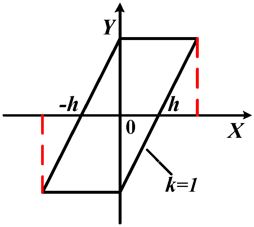
2.3.1. Dead Zone of Governor

The governors in the power system are all equipped with a certain dead zone, whose purpose is to reduce the frequent action of the governors caused by the frequency deviation in the power grid, so as to protect the governors and extend their service life. Due to the hysteresis and nonlinearity of the governor, the dead zone is generally described by the gap characteristic link. Figure 1 shows the characteristics of the governor’s dead zone, k is the slope. Assuming that the input of this nonlinear element is X and the output is Y, the relationship between the input and output is given in Equation (9) [22].

$$Y=F\left(X,\dot{X}\right)$$

(9)

When the function Y has a sinusoidal relationship, there is:

$$X=A\sin {\omega }_{0}t$$

(10)

where A is the amplitude of the sinusoidal input signal and ${\omega }_0$ is the frequency of the sinusoidal input signal. Linearize Y with the descriptive function method, then expand $F\left(X,\dot{X}\right)$ with the Fourier series, and take the first three terms:

$$F\left(X,\dot{X}\right)=F_0+N_{1}X+\left(N_2/{\omega }_0\right)\dot{X}$$

(11)

Among them, the various coefficients are:

$$\{\begin{array}{l}{F}^0=\frac{1}{2\pi }{\displaystyle {\int }_0^{2\pi }F\left(A\sin {\omega }_{0}t,A{\omega }_0\cos {\omega }_{0}t\right)d{\omega }_{0}t}\\ N_1=\frac{1}{\pi A}{\displaystyle {\int }_0^{2\pi }F\left(A\sin {\omega }_{0}t,A{\omega }_0\cos {\omega }_{0}t\right)\sin {\omega }_{0}td{\omega }_{0}t}\\ N_2=\frac{1}{\pi A}{\displaystyle {\int }_0^{2\pi }F\left(A\sin {\omega }_{0}t,A{\omega }_0\cos {\omega }_{0}t\right)\cos {\omega }_{0}td{\omega }_{0}t}\end{array}$$

(12)

By integrating the Equation (12), it can be obtained that each coefficient satisfies the following relationship:

$$\{\begin{array}{l}{F}^0=0\\ N_1=\frac{k}{\pi }\left[\frac{\pi }{2}+\arcsin \left(1-\frac{2h}{A}\right)+\left(1-\frac{2h}{A}\right)\sqrt{\frac{h}{A}\left(1-\frac{h}{A}\right)}\right],A\ge h\\ N_2=-\frac{4kh}{\pi A}\left(1-\frac{h}{A}\right),A\ge h\end{array}$$

(13)

where h is the dead zone setting value of the governor. When A = h, N₁ = N₂ = 0. When A/h increases, N₁ increases monotonically, and N₂ also increases after falling to A/h = 2. When A/h approaches infinity, N₁ and N₂ tend to be constant.

Substituting Equation (13) into Equation (11) and performing a Laplace change, combining with Equation (3), the transfer function of the governor with a dead zone after linearization can be obtained:

$$G_{\mathrm{g}}(\mathrm{s})=\frac{\left(N_2/{\omega }_0\right)s+N_1}{T_{g}s+1}$$

(14)

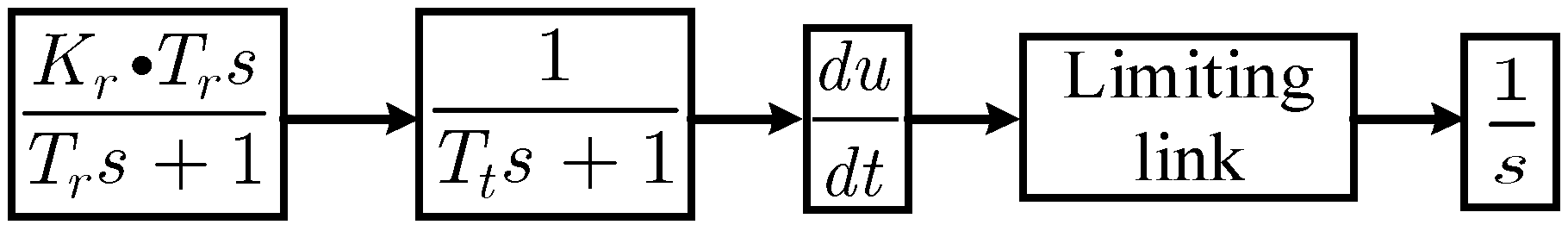
2.3.2. Generation Rate Constrains

GRC, also known as Unit Ramp Control (URC), refers to the unit output is limited by a certain maximum rate of change [23]. In the power grid, the given maximum change value is generally set as 0.0017 p.u.MW/s. In this paper, a limit device is added to the output variation of reheat steam turbine, and the limit device value is also 0.0017 p.u.MW/s. The reheat steam turbine model considering GRC is shown in Figure 2.

3. Model of Pumped Storage Power Station

3.1. Tie-Line Model

The tie-line is the transmission line that connects different grid areas. Ignoring the line loss, the flow power of the tie-line from area i to j can be expressed as [11]:

$$P_{tieij}=\frac{\left|V_i\right|\left|V_j\right|}{X_{ij}{P}_i^{\ast }}\sin \left({\theta }_i-{\theta }_j\right)$$

(15)

where P_tieij is the flow power of the tie-line; V_i, V_j are the voltage at both ends of the tie-line; θ_i, θ_j are the voltage angle at both ends of the tie-line; X_ij is the contact line circuit reactance; $P_i^{\ast }$ is the power of area i. The power micro-increment model of tie-line can be obtained from Equation (16), as given in Equation (17):

$$△\theta =2\pi {\displaystyle \int △f}dt$$

(16)

$$△P_{tieij}=2\pi \frac{\left|V_i\right|\left|V_j\right|}{X_{ij}{P}_i^{\ast }}\cos \left({\theta }_{i0}-{\theta }_{j0}\right)\left[{\displaystyle \int △f_i}dt-{\displaystyle \int △f_j}dt\right]$$

(17)

where △θ is the voltage angle micro-increment of the tie-line; △P_tieij is the power micro-increment of the tie-line; △f_i, △f_j are the frequency variation values of area i and j. The transfer function model of tie-line power deviation can be obtained by Laplacian variation of Equation (17), as given in Equation (18):

$$△P_{tieij}(s)=\frac{T_{ij}}{s}\left[△f_i(s)-△f_j(s)\right]$$

(18)

T_ij is defined as the contact line synchronization coefficient, and its calculation formula is given in Equation (19):

$$T_{ij}\triangleq 2\pi \frac{\left|V_i\right|\left|V_j\right|}{X_{ij}{P}_i^{\ast }}\cos \left({\theta }_{i0}-{\theta }_{j0}\right)$$

(19)

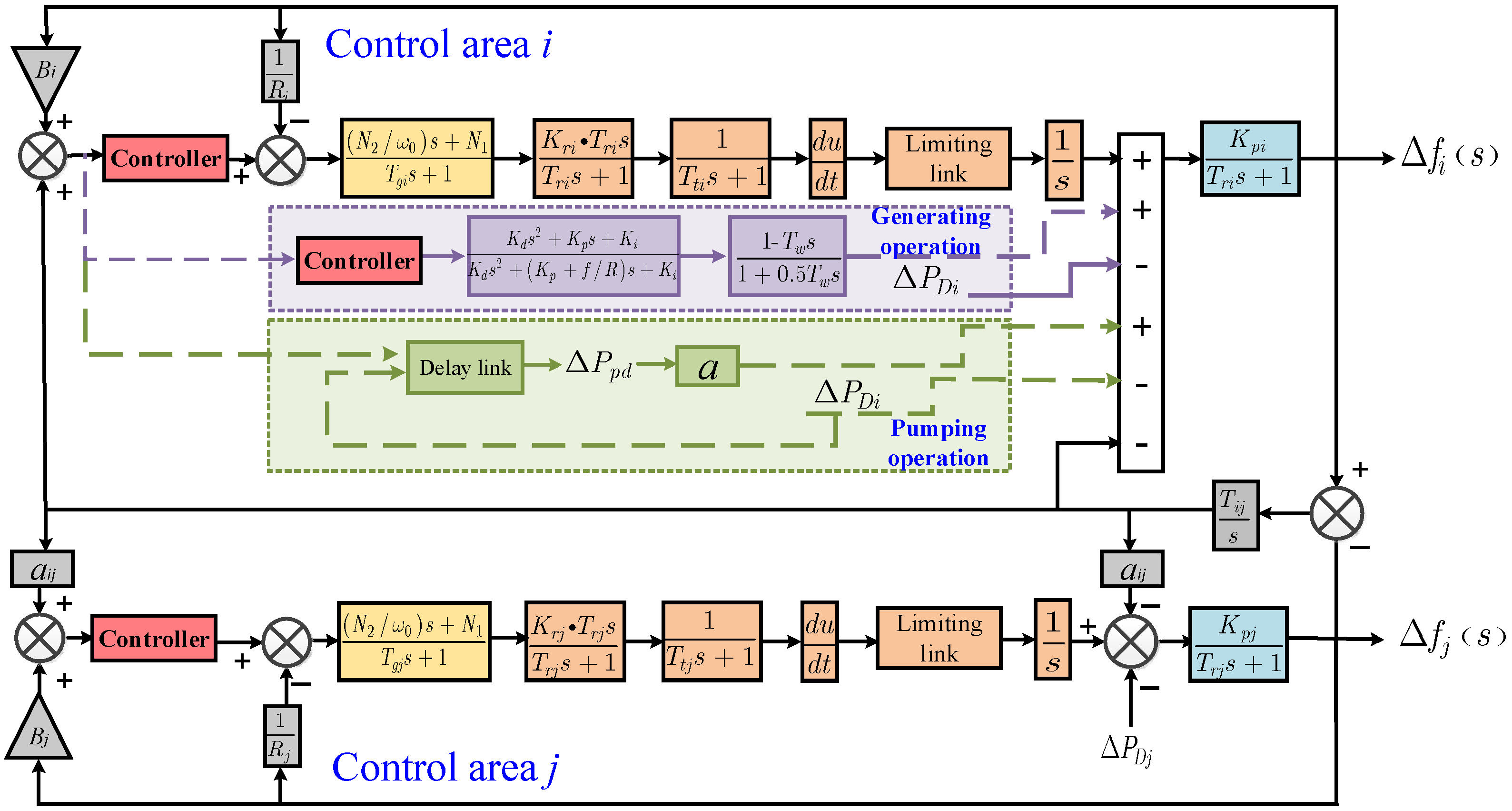
3.2. Two-Area LFC Model

The model of regional LFC system is obtained by combining the common component transfer functions described in detail in the previous section with the actual operation mode of the power grid. The LFC model with two single areas is connected with tie-lines to obtain the LFC model of the two-area reheat steam turbine with nonlinear links, as shown in Figure 3.

In the figure, ACE is used as the input, and the system frequency deviation is used as the output; △P_Di and △P_Dj are the load disturbance values exerted by area i and j; B is the Frequency deviation coefficient; a_ij is referred to as the synchronous power coefficient, which can be obtained from Equation (20).

$$a_{ij}=-P_j^{\ast }/P_i^{\ast }$$

(20)

where $P_i^{\ast }$ and $P_j^{\ast }$ are the rated power of the generator set in control area i and j respectively, and the parameters of tie-line are set is given in Equation (21).

$$T_{ij}=0.545, a_{ij}=-1,B=0.425$$

(21)

The transfer function relationship between generator and system connection in power grid is:

$$G_p(s)=\frac{△f(s)}{△P_g(s)-△P_d(s)}=\frac{1}{1+\frac{2H}{fD}s}\triangleq \frac{K_{pi}}{1+s{T}_{ri}}$$

(22)

where $K_{pi}\triangleq \frac{1}{D}$, $T_{ri}\triangleq \frac{2H}{fD}$, △P_g is the change of generator output power; △P_d is the change of load power; D is the load damping constant, which represents the load change caused by the change of unit frequency; H is the unit inertia constant defined by the standard value.

3.3. Model of Pumped Storage Power Station

Based on the fact that the main power plants in the power grid are all thermal power generation, the LFC model of pumped storage power station in this paper is based on the LFC model of reheat steam turbine in two-area, supplemented by the links of pumped storage power station. A two-stage pumped storage power model is established which can be divided into two basic operating conditions: generating operation and pumping operation. The generating operation is suitable for the peak load period. The hydraulic turbine operation causes the water flow in the upper reservoir to generate electricity in the lower reservoir, thus providing output for the power system. The pumping operation is suitable for the load trough period. At this time, the system relies on the surplus electricity to pump water from the lower reservoir, so as to reduce the output peak-valley difference of the power system, thus reducing the frequency of start and stop of the pumped storage units and the output variation, and maintaining the normal and stable operation of the units.

In this paper, the generating operation model of pumped storage power station is simplified as a hydraulic turbine unit, and the hydraulic turbine model simulation is used as an external power supply of the hydropower station. In pumping operation, it is equivalent to a load, considering the amount of power to support the grid when it stops pumping. Among them, the unit primary frequency regulation dead zone, ACE dead zone limit, maximum load adjustment limit and unit capacity limit are not considered. However, we consider some of the balance and constraints of the pumped storage power station:

Water balance of upper reservoir:

$$V_{ul}\left(t+1\right)=V_{ul}\left(t\right)-Q_t\left(t\right)$$

(23)

Balance of total generating water and total pumping water during the planning period:

$${\displaystyle \sum }_{t=1}^T{Q}_l\left(t\right)=V_{ul,0}-V_{ul,T}=0$$

(24)

Water balance of lower reservoir:

$$V_{dl}\left(t+1\right)=V_{dl}\left(t\right)+Q_t\left(t\right)$$

(25)

Flow limit under generating operation:

$$Q_{l,g.\min }\le Q_{l,g}\left(t\right)\le Q_{l,g.\max }$$

(26)

Flow limit under pumping operation:

$$Q_{l,pu.\min }\le Q_{l,pu}\left(t\right)\le Q_{l,pu.\max }$$

(27)

Capacity limit of upper reservoir:

$$V_{ul.\min }\le V_{ul}\left(t\right)\le V_{ul.\max }$$

(28)

Capacity limit of lower reservoir:

$$V_{dl.\min }\le V_{dl}\left(t\right)\le V_{dl.\max }$$

(29)

where Q is the water flow and V is the storage water volume of the reservoir. When the operation conditions of the pumped storage power station meet the above constraints, the two-stage pumped storage power model is established considering the two working states of generating and pumping operation of the pumped storage power station, is given in Equation (30). Structure diagram as shown in the dashed part of Figure 3.

$$G_p(s)=\{\begin{array}{l}△P_{pd}\\ G_d(s)G_t(s)\end{array}$$

(30)

where △P_pd is the power transmitted to the power grid when the pumping operation stops; G_d(s) is the transfer function model of hydraulic turbine governor under the generating operation, as given in Equation (4) or Equation (5); G_t(s) is the transfer function model of the hydraulic turbine, as given in Equation (2). In the Figure 3, a = {1,2…n}, n is the number of pumped storage units working under pumping operation.

4. Controller Design

The structure of the ADRC main components include: tracking differentiator (TD), extended state observer (ESO), and nonlinear state error feedback (NLSEF) [24]. However, the nonlinear form of ADRC needs to adjust multiple parameters, and these parameters affect each other. Based on the idea of ADRC, a linear auto disturbance rejection control (LADRC) method is proposed in [25], taking the controller bandwidth as the debugging parameter of the control performance. This method simplified the calculation, made it easy to set and maintain, and had the same control performance as traditional ADRC.

LADRC is composed of three important components: linear extended state observer (LESO), linear feedback control law, and disturbance compensation. Figure 4 shows the second-order LADRC structure adopted from [26], where r and y are the reference input and output of the system; G_p(s) is the controlled object; k_P and k_d are the linear feedback control rate parameters; d is the external disturbance of the system; and b₀ is the estimation of the input gain b of the system in the controller. The principle and function of each structure are introduced below.

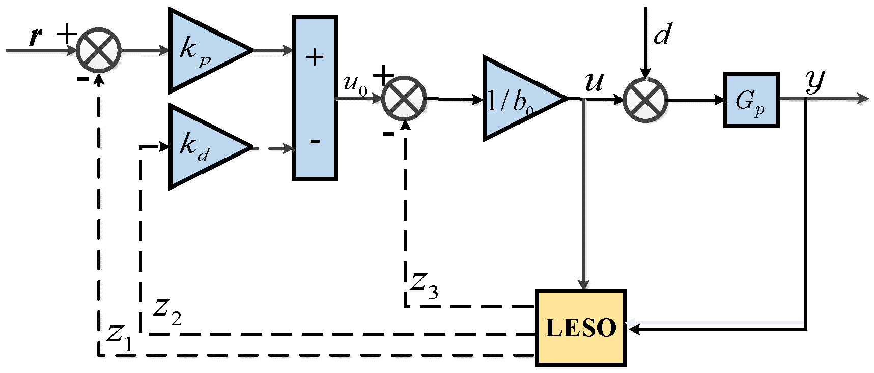
4.1. Linear Extended State Observer

LESO is the core part of the whole LADRC, which can observe the estimated values Z₁ and Z₂ of the state variable and the total disturbance Z₃ of the system according to the input and output data without relying on the specific mathematical model of generating disturbance.

The differential representation of the controlled second-order object G_p(s) is given in Equation (31):

$$\ddot{y}=g(y,\dot{y},w,t)+bu$$

(31)

where u is the controlled object input; y is the output; $\dot{y},\ddot{y}$ are the first and second order differentials of the output; w is the unmeasured disturbance of the system; b is the input gain; g is the total influence of the system’s own perturbation and external disturbance, and Equation (31) can also be expressed as:

$$\ddot{y}=l+b_{0}u$$

(32)

where l = g + (b − b₀) × u is the total disturbance of the system. Parameter b has a small range of change, and the approximate estimated gain value b₀ is used instead of b. At this time, the estimation error of b₀ on b is also regarded as part of the disturbance. When b₀ = b, it will not cause too much error to the observation state. Generally, take b₀ greater than b. Let x₁ = y, x₂ = $\dot{y}$, x₃ = l, l be defined as an expansion state of the system, the total disturbance of the system is expanded to a state variable x₃, so that the original second-order system is expanded into a new third-order linear system. Assuming that l is differentiable and ${\dot{x}}_3$ = h is defined, Equation (32) can be expressed in the state space as follows:

$$\{\begin{array}{l}{\dot{x}}_1=x_2\\ {\dot{x}}_2=x_3+b_{0}u\\ {\dot{x}}_3=h\\ y=x_1\end{array}$$

(33)

where x₁, x₂, x₃ are system state variables, h = $\dot{l}$. The estimated values of y, $\dot{y}$ and l can be obtained by using the LESO:

$$\{\begin{array}{l}{\dot{z}}_1=z_2+{\beta }_1\left(y-z_1\right)\\ {\dot{z}}_2=z_3+{\beta }_2\left(y-z_1\right)+b_{0}u\\ {\dot{z}}_3={\beta }_3\left(y-z_1\right)\end{array}$$

(34)

where z₁, z₂, z₃ are the estimated values of y, $\dot{y}$ and l, while β₁, β₂, β₃ are the gain parameters of the LESO to be determined to control the accuracy of the estimated values. Since the accuracy of the estimated value of the LESO is highly correlated with its bandwidth, let ω₀ be the bandwidth of the LESO, according to the work in [27], the observer gain parameters can be selected according to Equations (35) and (36):

$$\left[{\beta }_1,{\beta }_2,{\beta }_3\right]=\left[{\omega }_0{\alpha }_1,{{\omega }_0}^2{\alpha }_2,{{\omega }_0}^3{\alpha }_3\right]$$

(35)

$${\alpha }_i=\frac{\left(n+1\right)!}{i!\left(n+1-i\right)!}$$

(36)

Then the characteristic equation of LESO can be configured into the form of Equation (37):

$${\lambda }_0=s^3+{\beta }_1{s}^2+{\beta }_{2}s+{\beta }_3={(s+{\omega }_0)}^3$$

(37)

The parameterized gain coefficient of LESO is expressed as:

$$\{\begin{array}{l}{\beta }_1=3{\omega }_0\\ {\beta }_2=3{{\omega }_0}^2\\ {\beta }_3={{\omega }_0}^3\end{array}$$

(38)

Therefore, ω₀ is the only parameter to be adjusted in the LESO. This configuration can not only ensure the stability of the system, but also give a better transition process, which makes the calculation easy. The range of values takes into account the controllability and noise resistance of the system. After ω₀ is determined, β₁, β₂, β₃ can be determined correspondingly according to Equation (38) [28].

4.2. Disturbance Compensation

As shown in Figure 4, the disturbance compensation link is set as follows:

$$u=\frac{u_0-z_3}{b_0}$$

(39)

where u₀ is the virtual control amount. If the LESO can achieve z₃ = l, the Equation (39) is brought into the Equation (32), and $\ddot{y}$ = u₀ is obtained, that is, the controlled object is converted into a double integrator series structure for easy control.

4.3. Linear Feedback Control

NLSEF calculates the control signal u₀ according to the system state error. The following proportional higher order differential control rate is used:

$$u_0=k_p\left(r-z_1\right)-k_d{z}_2$$

(40)

Reference [29,30] analyzed the stability of LADRC in uncertain time-varying systems, and introduced that LADRC can achieve the following two goals: One is the convergence of the closed-loop system, and the other is that the dynamic performance of the closed-loop system can be optimized by adjusting the bandwidth of LESO. With closed-loop stability, the closed-loop equation of the control system can be obtained as given in Equation (41) by introducing Equation (40) into the double integrator series object Equation (39) after the disturbance compensation.

$$\ddot{y}+k_d\dot{y}+k_{p}y=k_{p}r$$

(41)

By using the relationship between bandwidth and control performance, the characteristic polynomial of closed-loop Equation (41) is expressed in the form of ω_c as given in Equation (42) if ω_c is the controller bandwidth.

$${\lambda }_0=s^2+k_{d}s+k_p={(s+{\omega }_c)}^2$$

(42)

The controller parameters can be expressed as:

$$\{\begin{array}{l}{k}_p={{\omega }_c}^2\\ k_d=2{\omega }_c\end{array}$$

(43)

ω_c is the only parameter to be set in the controller, which simplifies the calculation of controller parameters. The value ranges between the response speed and stability of the system [27]. The values of k_d and k_P are determined according to the relationship between Equation (43) and ω_c.

5. The Simulation Analysis

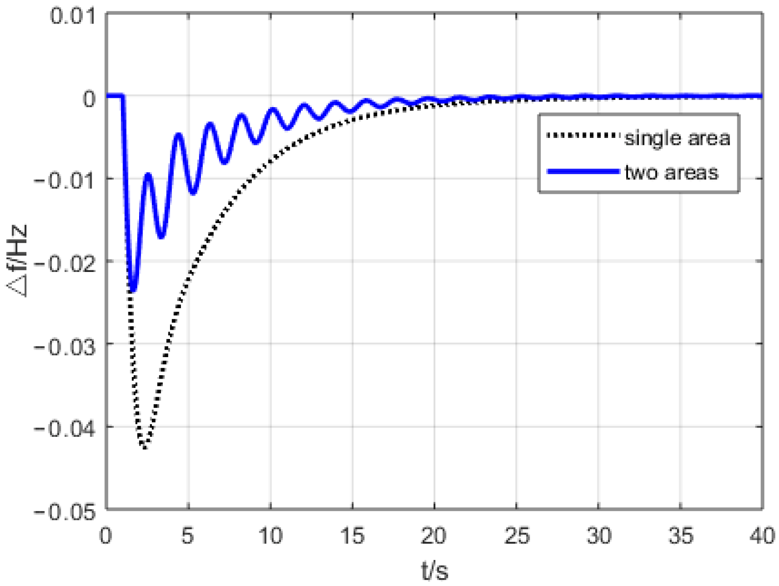
5.1. Simulation of Load Frequency Control in Single and Two-Area

In this paper, first of all, the LFC models of single-area and two-area reheat steam turbine units are established by MATLAB/Simulink (MATLAB R2018b, Math Works, Natick, MA, USA, 1984). FFC mode is adopted for single-area ACE, and TBC mode is adopted for two-area ACE. According to the model parameters of reheat steam turbine and generator power system in [15], the LFC parameters of reheat steam turbine unit in the two-area in this paper are obtained as shown in

Table 1. Basic parameters of the regional load frequency control (LFC) model for reheat steam turbine unit.

Parameters	Value	Parameters	Value
Tgi	0.08 s	Tri	10 s
Tti	0.3 s	Tpi	20 s
Kri	0.5	Kpi	120
Ri	2.4

, and the control simulation module of regional reheat steam turbine unit is determined to reflect the corresponding frequency changes. The unit parameter values in the two-area are set consistently and the parameters of tie-line are given in Equation (21). A disturbance signal of 0.01 p.u.MW is added to area i at 1 s. The frequency variation chart of the single and two-area is shown in Figure 5.

The simulation results are shown in Figure 5. It can be seen from the simulation diagram that the system is disturbed at 1s, and the frequency decreases rapidly. The maximum frequency variation of the two-area is nearly 50% less than that of the single-area. The regulation time of the two-area is shortened by 5 to 6 s, which can restore to the stable state more quickly, but the frequency oscillation frequency increases. It can be seen that when a disturbance occurs in region i, the interconnected region j can provide power support to region i through tie-lines, helping the disturbed region to restore the frequency to a stable state more quickly. Compared with isolated network operation, the safety and stability of large power grid model are improved.

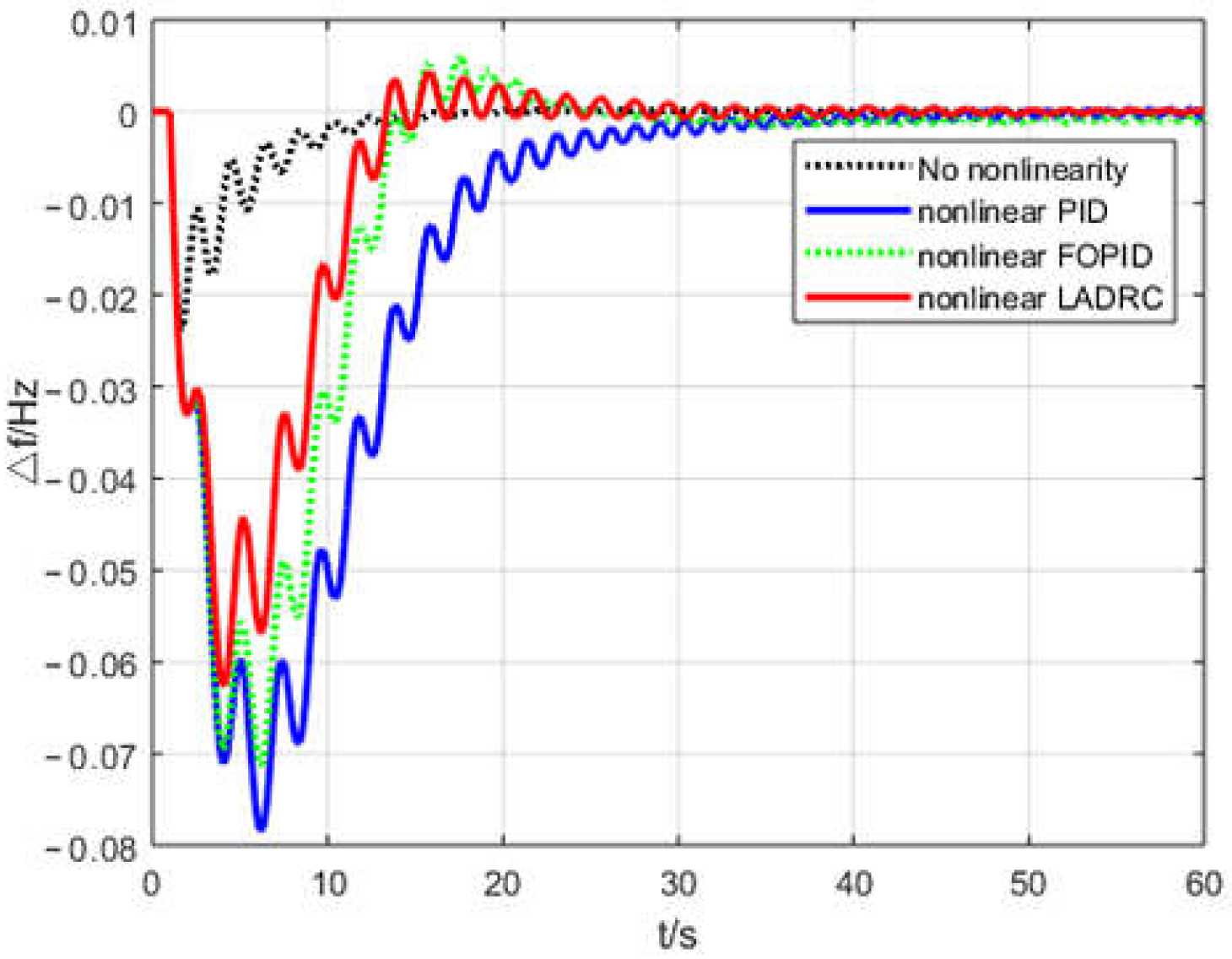
5.2. Simulation of Two-Area LFC Considering Nonlinearity

A two-area reheat steam turbine LFC model with nonlinear links is established as shown in Figure 3 (without dashed line part). The parameters of the unit model, tie-line and regional disturbance are set up in accordance with the previous section. The controller adopts traditional PID, FOPID, and LADRC. According to the parameter design of the controllers in [26], the cut-and-trial method is used to determine and select the LFC parameters suitable for the pumped storage power station in this paper, so as to effectively suppress the disturbance and restore the frequency stability. Its control parameters are given in

Table 2. Basic parameters of controller.

Controller	Parameters	Value	Parameters	Value
Traditional proportion integration differentiation (PID)	Kp	5	Ki	0.5
	Kd	1
fractional-order proportion integration differentiation (FOPID)	Kp	37	Ki	7
	Kd	8	λ	0.08
	µ	0.055
linear active disturbance rejection control (LADRC)	Kp	49	Kd	14
	ω0	1.1	ωc	7
	b	290	d	0

, and the simulation time domain is 60 s. The frequency variation chart of the disturbance zone under different controllers is shown in Figure 6.

The simulation results are shown in Figure 6. It can be seen from the figure that, after taking nonlinear factors into consideration, the amplitude of frequency variation of the system greatly increases to more than 3 times of the original value, and the frequency recovery speed also decreases. The reason is that the speed constraint of steam turbine in nonlinear factors restricts the rapid output of the units, resulting in the lack of power cannot be compensated in time, and the frequency recovery is slow. Compared with the three different controllers, LADRC has the best control effect, with the smallest frequency oscillation range and the shortest recovery time. The amplitude of oscillation decreases to approximately 0.016 Hz, and the recovery time is shortened nearly 20 s. The second is FOPID, and the worst is the traditional PID. The correctness and validity of the LADRC method proposed in this paper are verified.

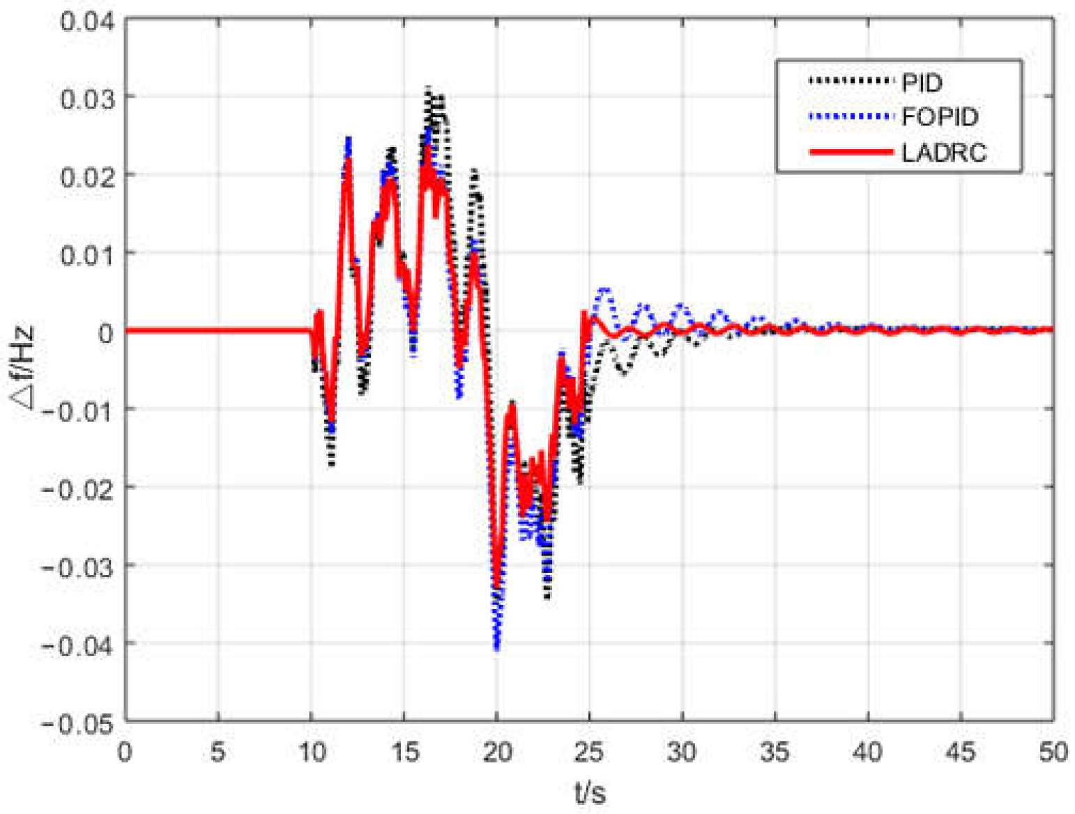
5.2.1. Simulation of LFC under Random Disturbance

Considering the influence of random factors in the actual situation, disturbances are mostly unmeasured and uncertain clutter. Therefore, considering that the random disturbance time is between 10 s and 25 s, the disturbance amplitude is [−0.01 p.u.MW, 0.01 p.u.MW], and the simulation time domain is 50 s, the performance of LADRC, FOPID and traditional PID controller under uncertain disturbance is observed. The simulation results are shown in Figure 7. At this time, the frequency is affected and oscillates constantly. However, LADRC has the shortest regulation time and the fastest recovery speed, and tends to be stable after 25 s. It can be seen from the oscillation amplitude that it is smaller than the other two controllers. It can be seen that LADRC proposed in this paper still has excellent control performance under unpredictable and irregular disturbances.

5.2.2. Stability and Robustness Analysis of Different Control Methods

In this section, we evaluate various control methods in the form of tables under different error criteria.

Table 3. Error evaluate of controllers under load disturbance.

Controller	Disturbance Duration (s)	Maximum Amplitude (Hz)	Overshoot (Hz)	MSE (× 10−4)
Traditional PID	24	0.035	0	6.19
FOPID	26	0.041	0.005	5.30
LADRC	17	0.033	0.003	3.85

comprehensively analyzes the simulation results of Figure 7, compares the influence of three control methods on frequency control results under load disturbance, and evaluates the stability and robustness of the three methods.

As shown in Table 3, we select the four dimensions of disturbance duration, maximum amplitude, overshoot and mean square error (MSE) to evaluate the controller error. It is obvious that LADRC has the shortest disturbance time, the smallest maximum amplitude and MSE among the three. Compared with traditional PID, LADRC and FOPID have overshoot, but the overshoot is within the allowable range. Moreover, the MSE of LADRC is quite different from that of other controllers, compared with the traditional PID is 6.19, LADRC is only 3.85, almost double the relationship, which shows that LADRC has better control accuracy. Therefore, the anti-disturbance capability of LADRC is more remarkable. The disturbance time of FOPID is only 2 seconds slower than that of traditional PID, which is nearly the same, and its maximum amplitude is higher, but the MSE of observation is much smaller than the traditional PID. The comprehensive analysis shows that the FOPID data has a low degree of variation and a small error. Although the control effect is higher than the traditional PID, compared with LADRC, there is still a large disparity.

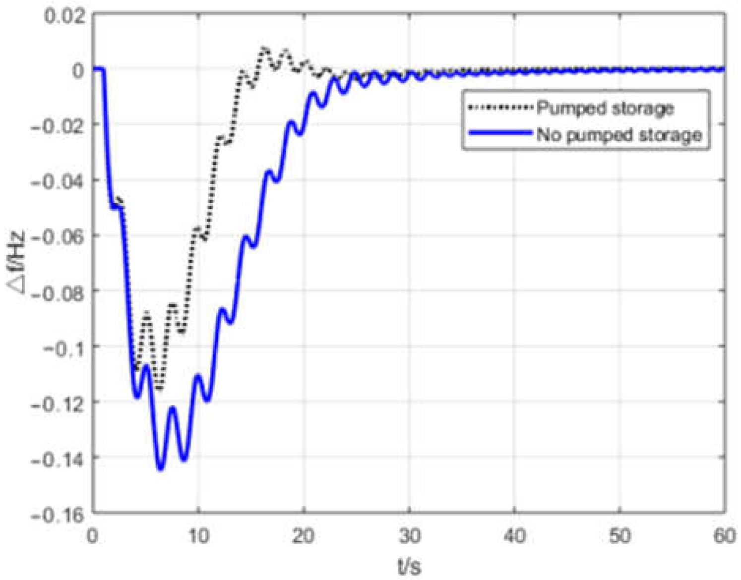
5.3. LFC Simulation of Pumped Storage Power Station

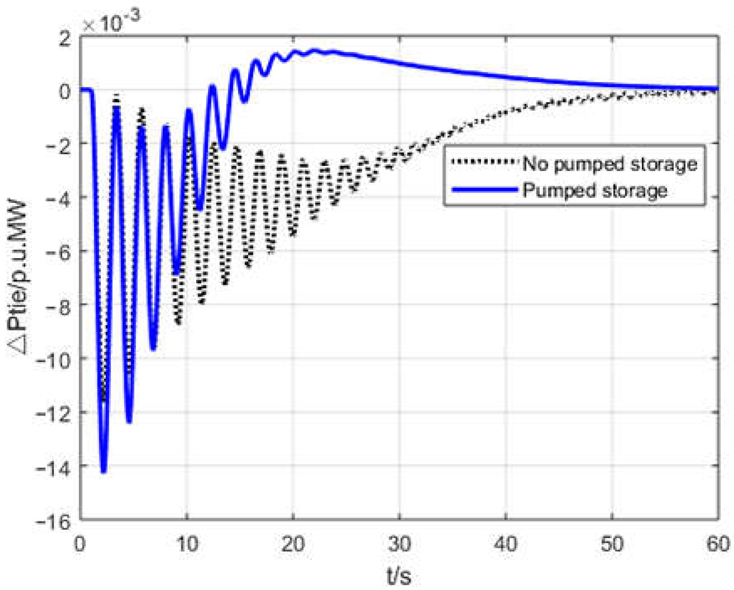
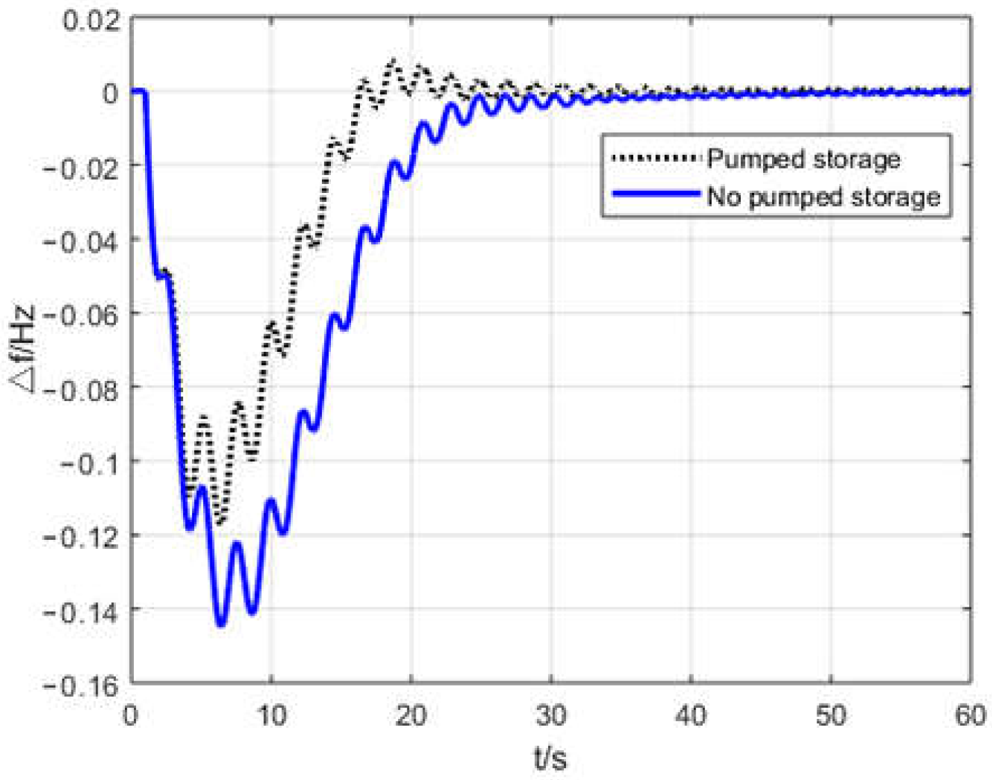
5.3.1. Generating Operation

Based on the LFC of reheat steam turbine, this paper builds the pumped storage energy LFC model under generating operation according to the dashed line in Figure 3. DEH is adopted as the governor of hydraulic turbine. The LADRC designed in this paper is adopted as the controller. According to the model parameters of hydraulic turbine in [15], the LFC parameters of the hydraulic turbine unit in this paper are shown in

Table 4. Basic parameters of hydraulic turbine.

Parameters	Value	Parameters	Value
Twi	1 s	Kd	4
Ki	5
Kp	1

. It is determined that the frequency control simulation parameters of generating and pumping operation in this paper can reflect the corresponding frequency changes, so as to achieve the analogue simulation of frequency modulation function of pumped storage power station. The simulation time domain was set to 60 s, and a disturbance of 0.015 p.u.MW occurred in the system at 1 s. The frequency variation chart of the disturbance zone when the pumped storage power station works in the generating operation is shown in Figure 8, and the exchange power chart of the tie-line is shown in Figure 9.

Since the pumped storage power station working in the generating operation has been added to the hydraulic turbine, which is almost free from the restriction of GRC and can rapidly increase its output to make up for the power loss caused by the disturbance of the system, thus accelerating the frequency stability. Figure 8 intuitively shows that the maximum value of grid frequency decline is significantly reduced, and the recovery time is shortened by nearly 10 s. It can be seen that the frequency control of the disturbance zone after the pumped storage power station is more robust to interference, and the reliability of the LADRC method is further verified. From the change of the exchange power of the tie-line, after the pumped storage energy is added, the exchange power of the tie-line increases, then decreases, and its recovery speed is obviously accelerated. Due to the accelerated frequency recovery speed, the power of the tie-line inevitably produces certain overshoot, but the overshoot is within the allowable range.

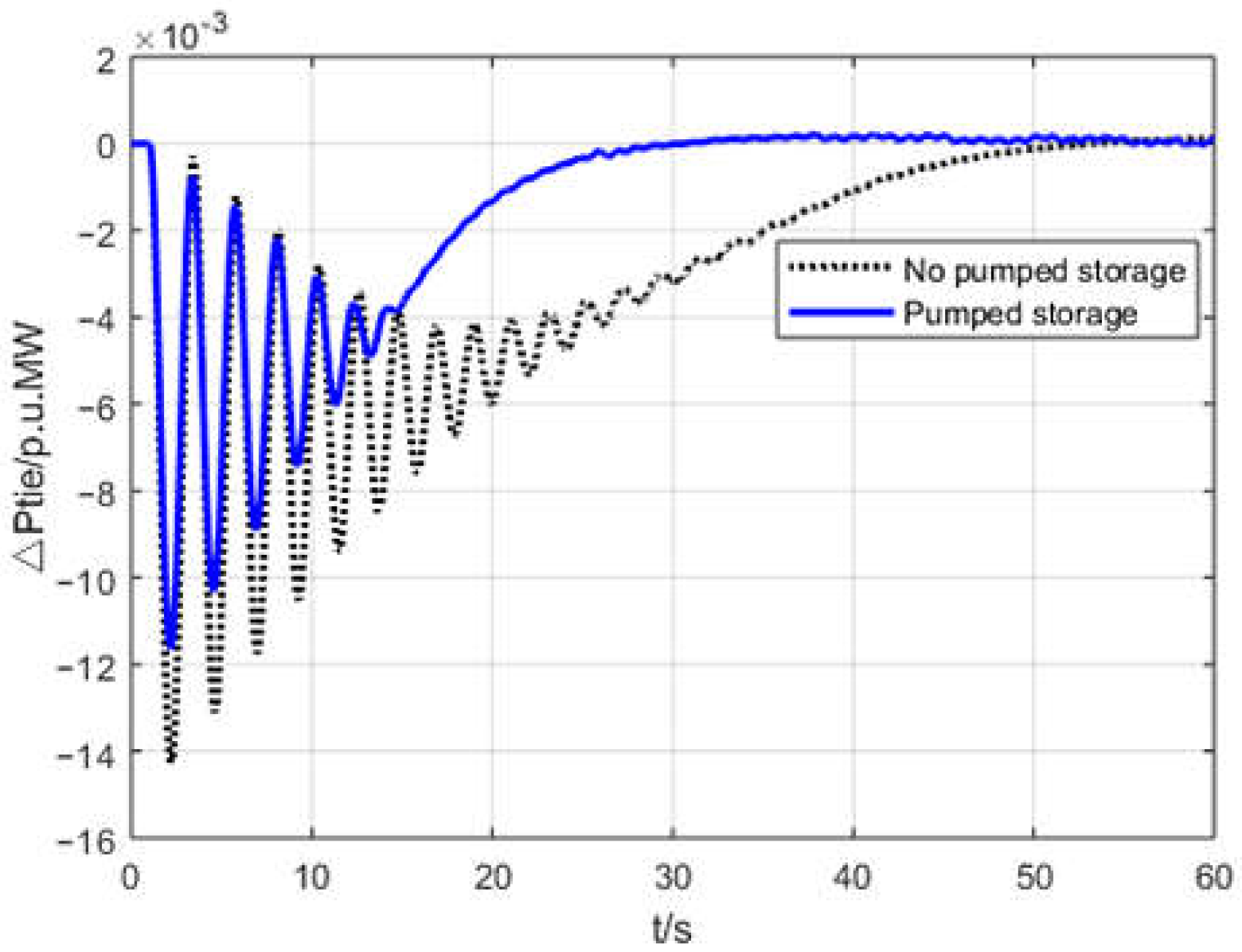
5.3.2. Pumping Operation

The LFC model of the pumped storage power station under pumping operation is established according to the dashed line in Figure 3. The pumping power is set at 0.05, △P_pd = 0.05, a = 1. The parameter setting is consistent with the last section of the generating operation. The frequency variation chart of the disturbance zone is shown in Figure 10, and the exchange power chart of the tie-line is shown in Figure 11.

When load disturbance occurs in the pumping operation, the pumped storage power station can stop pumping after receiving the signal from the grid, cut off part of the load quickly, and support the power consumed by pumping to the grid to maintain the stability of the grid frequency. From the simulation results, it can be seen that the pumped storage power station working under the pumping operation obtains certain power support in a short time after the grid disturbance, and the frequency fluctuation range is shortened and restored to the stable state more quickly and smoothly. For the exchange power of the tie-line, the pumping operation reduces the value of the exchange power, significantly reduces the number of oscillations and amplitude. The recovery rate is more than twice that of without pumped storage energy, which is an effective supplement to the LFC of the power grid.

6. Conclusions

In this paper, an LFC method for a pumped storage unit based on LADRC is proposed. Firstly, the LFC of reheat steam turbine with nonlinear factors is modeled, and according to the working mode of the pumped storage power station, the power plant LFC model under generating and pumping operations is established. The following conclusions are obtained from the simulation results: (1) After the regional combination, the anti-interference ability of the system is strengthened, and power support can be obtained from the uninterrupted area of the interconnection, so as to better maintain the safe and stable operation of the power grid. (2) The LADRC method proposed in this paper can achieve better control effect and better robustness than FOPID and traditional PID control when controlling pumped storage power stations with nonlinear links. (3) It is effective and feasible to introduce the pumped storage power station into the LFC, which greatly improves the dynamic characteristics of the LFC of the power grid.

References

1. Shi, Z.; Li, Q.; Huang, B.; Hong, B. Research on distributed energy storage operation mode and technical economy under the background of energy internet. IOP Conf. Ser. Mater. Sci. Eng. 2019, 486, 012077. [Google Scholar] [CrossRef]
2. Sinsel, S.; Riemke, R.L.; Hoffmann, V.H. Challenges and solution technologies for the integration of variable renewable energy sources—A review. Renew. Energy 2020, 145, 2271–2285. [Google Scholar] [CrossRef]
3. Laghari, J.; Mokhlis, H.; Abu Bakar, A.H.; Mohamad, H. A fuzzy based load frequency control for distribution network connected with mini hydro power plant. J. Intell. Fuzzy Syst. 2014, 26, 1301–1310. [Google Scholar] [CrossRef]
4. Pérez-Díaz, J.I.; Sarasúa, J.I.; Wilhelmi, J.R. Contribution of a hydraulic short-circuit pumped-storage power plant to the load–frequency regulation of an isolated power system. Int. J. Electr. Power Energy Syst. 2014, 62, 199–211. [Google Scholar] [CrossRef]
5. Singh, V.P.; Samuel, P.; Kishor, N. Impact of demand response for frequency regulation in two-area thermal power system. Int. Trans. Electr. Energy Syst. 2016, 27, e2246. [Google Scholar] [CrossRef]
6. Li, J.; Sun, W.; Shi, Y.; Li, H.; Li, W.; Li, N.; Hua, F. Optimization and promotion of automatic generation control strategy under large-scale wind power. IOP Conf. Ser. Earth Environ. Sci. 2018, 186, 012026. [Google Scholar] [CrossRef] [Green Version]
7. Plotnikova, T.V.; Sokur, P.V.; Tuzov, P.Y.; Shakaryan, Y.G.; Kuleshov, M.A. Participation of a pumped-storage electric power plant with asynchronous generator-motors in normalized primary frequency regulation. Power Technol. Eng. 2015, 49, 223–228. [Google Scholar] [CrossRef]
8. Wu, C.-C.; Lee, W.-J.; Cheng, C.-L.; Lan, H.-W. Role and value of pumped storage units in an ancillary services market for isolated power systems—Simulation in the Taiwan power system. IEEE Trans. Ind. Appl. 2008, 44, 1924–1929. [Google Scholar] [CrossRef]
9. Papaefthymiou, S.V.; Karamanou, E.G.; Papathanassiou, S.A.; Papadopoulos, M.P. A wind-hydro-pumped storage station leading to high RES penetration in the autonomous island system of Ikaria. IEEE Trans. Sustain. Energy 2010, 1, 163–172. [Google Scholar] [CrossRef]
10. Jin, Z.; Xu, L.; Ningbo, W. Study on control of pumped storage units for frequency regulation in power systems integrated with large-scale wind power generation. Proc. CSEE 2017, 37, 564–571. [Google Scholar]
11. Fosha, C.; Elgerd, O. The megawatt-frequency control problem: A new approach via optimal control theory. IEEE Trans. Power Appar. Syst. 1970, 4, 563–577. [Google Scholar] [CrossRef]
12. Nanda, J.; Mangla, A. Automatic generation control of an interconnected hydro-thermal system using conventional integral and fuzzy logic controller. In Proceedings of the 2004 IEEE International Conference on Electric Utility Deregulation, Restructuring and Power Technologies, Hong Kong, China, 5–8 April 2004; pp. 372–377. [Google Scholar]
13. Han, J. From PID to active disturbance rejection control. IEEE Trans. Ind. Electron. 2009, 56, 900–906. [Google Scholar] [CrossRef]
14. Han, W.; Wang, G.; Stankovic, A.M. Active Disturbance Rejection Control in fully distributed Automatic Generation Control with co-simulation of communication delay. Control. Eng. Pr. 2019, 85, 225–234. [Google Scholar] [CrossRef]
15. Dong, L.; Zhang, Y.; Gao, Z. A robust decentralized load frequency controller for interconnected power systems. ISA Trans. 2012, 51, 410–419. [Google Scholar] [CrossRef] [PubMed] [Green Version]
16. Tan, W.; Hao, Y.; Li, N. Load frequency control in deregulated environments via active disturbance rejection. Int. J. Electr. Power Energy Syst. 2015, 66, 166–177. [Google Scholar] [CrossRef]
17. Liu, F.; Li, Y.; Cao, Y.; She, J.; Wu, M. A two-layer active disturbance rejection controller design for load frequency control of interconnected power system. IEEE Trans. Power Syst. 2016, 31, 3320–3321. [Google Scholar] [CrossRef]
18. Tan, W.; Chang, S.; Zhou, R. Load frequency control of power systems with non-linearities. IET Gener. Transm. Distrib. 2017, 11, 4307–4313. [Google Scholar] [CrossRef]
19. Alomoush, M.I. Load frequency control and automatic generation control using fractional-order controllers. Electr. Eng. 2010, 91, 357–368. [Google Scholar] [CrossRef]
20. Çam, E. Application of fuzzy logic for load frequency control of hydro electrical power plants. Energy Convers. Manag. 2007, 48, 1281–1288. [Google Scholar] [CrossRef]
21. Nanda, J.; Sharma, D.; Mishra, S. Performance analysis of automatic generation control of interconnected power systems with delayed mode operation of area control error. J. Eng. 2015, 2015, 164–173. [Google Scholar] [CrossRef]
22. Singh, O.; Nasiruddin, I. Hybrid evolutionary algorithm based fuzzy logic controller for automatic generation control of power systems with governor dead band non-linearity. Cogent Eng. 2016, 3, 1161286. [Google Scholar] [CrossRef]
23. Das, D.; Nanda, J.; Kothari, M.L.; Kothari, D.P. Automatic generation control of a hydrothermal system with new area control error considering generation rate constraint. Electr. Mach. Power Syst. 1990, 18, 461–471. [Google Scholar] [CrossRef]
24. Shen, Z.; Zhiqiang, G. Active disturbance rejection control for non-minimum phase systems. In Proceedings of the 29th China control conference, Beijing, China, 29–31 July 2010. [Google Scholar]
25. Gao, Z. Active Disturbance Rejection Control: A paradigm shift in feedback control system design. In Proceedings of the American Control Conference IEEE, Minneapolis, MN, USA, 14–16 June 2006. [Google Scholar]
26. Liu, K.; He, J.; Luo, Z.; Shen, X.; Liu, X.; Lu, T. Secondary frequency control of isolated microgrid based on LADRC. IEEE Access 2019, 7, 53454–53462. [Google Scholar] [CrossRef]
27. Fang, J.; Tan, W.; Fu, C. Analysis and tuning of linear active disturbance rejection controller for load frequency control of power systems. In Proceedings of the 32nd Chinese Control Conference IEEE, Xi’an, China, 26–28 July 2013; pp. 5560–5565. [Google Scholar]
28. Gao, Z. Scaling and bandwidth-parameterization based controller tuning. In Proceedings of the 2003 American Control Conference, Denver, CO, USA, 4–6 June 2003; Volume 6, pp. 4989–4996. [Google Scholar]
29. Zheng, Q.; Gao, L.Q.; Gao, Z. On stability analysis of active disturbance rejection control for nonlinear time-varying plants with unknow dynamics. In Proceedings of the 46th IEEE Conference on Decision and Control, New Orleans, LA, USA, 12–14 December 2007. [Google Scholar]
30. Wenchao, X.; Yi, H. The active disturbance rejection control for a class of MIMO block lower-triangular system. In Proceedings of the IEEE 30th Chinese Control Conference (CCC 2011), Yantai, China, 22–24 July 2011; pp. 6362–6367. [Google Scholar]
Figure 1. Dead zone characteristics of governor.
Processes 08 00380 g001
Figure 2. Reheat steam turbine model considering Generation Rate Constrains (GRC).
Processes 08 00380 g002
Figure 3. Pumped storage power station model.
Processes 08 00380 g003
Figure 4. Second-order linear active disturbance rejection control (LADRC) structure diagram.
Processes 08 00380 g004
Figure 5. Single and two-area frequency variation chart of reheat steam turbine.
Processes 08 00380 g005
Figure 6. Frequency variation chart of the disturbance zone under different controllers.
Processes 08 00380 g006
Figure 7. The system frequency variation chart under random disturbance.
Processes 08 00380 g007
Figure 8. Frequency variation chart of the disturbance zone at generating operation mode.
Processes 08 00380 g008
Figure 9.Ptie variation chart at generating operation mode.
Processes 08 00380 g009
Figure 10. Frequency variation chart of the disturbance zone at pumping operation mode.
Processes 08 00380 g010
Figure 11.Ptie variation chart at pumping operation mode.
Processes 08 00380 g011