1. Introduction
This article reconsiders the Q-learning method for quadratic optimal control problem of discrete-time linear systems. Therefore, it is necessary to explain the quadratic optimal control problem of discrete-time linear systems. There is a discrete-time linear system which can be described as , where is states of system, is the control value, is state matrix, is control matrix. The quadratic optimal control problem for the system is to minimize the quadratic performance index function , by designing a proper state feedback matrix and choosing control law . According to the optimal control theory, the optimal value of feedback matrix should satisfy following equation: , where the matrix should be the solution of Riccati equation . So, if matrices and are known, by setting proper matrices and , and resolving matrix from Riccati equation, the optimal feedback matrix can be solved. It can be seen from the above process that the precondition of the calculation process is the precise acquaintance of controlled systems’ mathematical models.
There are great amount of papers which discussed the design of model-free controllers via Q-learning method for linear discrete-time systems, while the independence of data during the computation process is not get enough attention. In this paper, the effect of the data correlation is discussed, specifically aiming to the computation processes of optimal controllers for linear discrete-time systems adopting Q-learning method. Based on the theoretical analysis, the data independence condition should be satisfied to implement the existing Q-learning method. The data sets sampled from the linear discrete-time systems is destined relevant, which means that the controllers cannot be solved by the existing Q-learning method. To design proper controllers for linear discrete-time systems, an improved Q-learning method is proposed in this paper. The improved method adopts the ridge regression instead of the least squares regression. The ridge regression can deal with the multiple collinearity of the sample sets. Therefore, the proper controllers can be solved by the proposed method.
In this paper, following results have been achieved. First, limited to linear discrete-time systems, the computation process cannot be executed correctly by the existing Q-learning method. Second, relative corollaries have been made for several types of systems, to indicate in detail the necessary for data independence condition for different situations. Third, an improved Q-learning method has been proposed to solve the problem of multiple collinearity. At last, results of simulations show the effectiveness of the proposed method.
2. Q-Learning Method for Model-Free Control Schemes
Generally, there is an obvious difference between optimal control [
1] and adaptive control [
2,
3]. Adaptive controller often needs online dynamic data of systems. On the contrary, optimal controllers are designed off-line by solving Hamilton-Jacobi-Bellman (HJB) equations. In optimal theory, the solution of HJB equations is the real valued function with minimum cost for specific dynamic system and corresponding cost function. Therefore, the solution of HJB equations is also the optimal controller of the controlled system. In the HJB equations, all information of the controlled system should be known, which means the precise mathematical model of the system should be established. To solve HJB equations, many methods have been researched, and the earlier mentioned Riccati equation is derived from HJB equations. According former expoundation, the optimal controller cannot be designed under model-free condition. However, the development of theory made the combination of the two different control schemes. The reinforcement learning theory plays an important part in the process.
As one of the most important reinforcement learning methods, Q-learning has been proved by Watkins [
4] that under certain conditions the algorithm converges to the optimum cation-values. Therefore, the calculation of optimal controllers became realizable for complete or partial model-free systems by adopting online calculation method. With data sets sampled from systems, optimal controllers can be designed by Q-learning method. Many researchers took the view and many achievements have been made. Compared with other popular techniques such as SVM and KNN [
5], reinforcement learning methods represented by Q-learning are unsupervised algorithms. They do not need the target information of the train data, on the contrary, they evaluate their actions by the value functions aiming to the current status. Their directions of calculation are decided by the value functions, in this sense, the reinforcement learning methods are also gradient-free optimization methods [
6] when they are used to solve optimization problems. Some optimal estimation algorithms such as Kalman filter and its extended forms [
7] have been adopted by many researchers as observers in adaptive control schemes. Their observation results still rely on the structure and parameters of systems, so these algorithms are beyond the boundary of model-free methods.
Bradtke used the Q-learning method to solve quadratic control problem for discrete-time linear systems [
8]. He set up the model-free quadratic optimal control solution based on data, and studied the convergence of Q-learning method for certain type of systems. From then on, the important position of Q-learning in model-free quadratic optimal control is established. And the Q-learning schemes for the continuous-time systems also had been proposed [
9,
10], without the convergence condition.
As a kind of typical data-based iterative algorithm, Q-learning method has been used to solve problems in many fields, including but not limited to following examples. An adaptive Q-learning algorithm is adopted to obtain the optimal solution between exploration and exploitation of electricity market [
11]. An effective Q-learning algorithm is proposed to solve the traffic signal control problem [
12], and satisfying results have been obtained. A distributed Q-learning (QD-learning) [
13] algorithm is investigated to get the solution of the sensor networks collaboration problem. A time-based Q-learning algorithm is adopted to get the optimal control of the energy systems [
14,
15].
Compared with other fields, the quadratic optimal control problems attract main attention in this paper. To design feedback controllers for discrete and continuous-time systems, the principles of using reinforcement learning method are fully described [
16]. According to the paper, reinforcement learning method of policy iteration and value iteration can be used to design adaptive controllers which converge to the optimal control theory. Adopting Q-learning schemes for adaptive linear quadratic controllers [
17], the difference between linear and nonlinear discrete-time systems has been compared. Simulations show that controllers for both kind of the systems can be solved with almost same convergence speed. Some researchers focused on output feedback control schemes [
18,
19,
20,
21]. The method to design optimal or nearly optimal controllers has been studied for linear discrete-time systems subject to actuator saturation condition [
21,
22,
23,
24]. Other researchers considered stochastic linear quadratic optimal control as an effective method [
25,
26,
27,
28].
3. Problem Description and Improved Method
Theoretically, the existing Q-learning algorithm can calculate optimal or approximate optimal controllers as a model-free method. For discrete-time linear systems, there is an obvious limitation caused by multi-collinearity of data sets sampled from systems, which is shown by analysis. To solve the problem, the existing Q-learning algorithm need to be modified, as the same situation as the existing stability analysis method for uncertain retarded systems [
29]. By adopting ridge regression, an improved algorithm has been proposed in this paper, which can overcome the multi-collinearity problem and obtain the proper controller. To explain the limitation of the existing Q-learning method, the design principle of the existing Q-learning model-free quadratic optimal controllers is shown in following section.
3.1. Design Process of Quadratic Optimal Controller by Existing Q-Learning Method
To design a quadratic optimal controller, a linear discrete-time system is considered to be:
where
is a vector of state variables,
is control input vector,
is
state matrix,
is input
matrix. And
is a complete controllability pair. There is the single step performance index is expressed as:
where
is
weight matrix,
is
weight matrix,
is complete observability pair,
is discount factor. Please note that:
The problem of quadratic optimal control can be described as follows. For system formed as Equation (
1), a control law
should be designed to minimize
. Based on Formula (3),
means the total performance index for infinite time quadratic control systems. To minimize the total performance index, the Q function is defined as:
Formula (4) shows that the Q function is not a new function but just another expression of total performance index
. Then the Q function can be calculated as following formula:
The feedback law can be calculated by following formula according to the extremum condition of
,which is
.
where
is the solution of Riccati equation:
And should satisfy following equation: .
The design method of model-based controller is that the control law will be established by solving Equation (
7). According to the optimal control theory, the values of the matrices and will decide the different weights between the quantity of states and control values [
26]. The values of matrices of
Q and
R often depend on performance index, experience of designers and constraint conditions. The quadratic optimal controller based on Q-learning is model-free, and shown as follows. Equation (
5) is represented as:
where
, and the parameters vector
. The Q function possesses the recurrence relation shown by following formula:
Therefore, the following formula can be deduced:
There are N equations formed by Formula (10) can be built if sets of data on state and control have been collected. Please note that:
With the least squares method, the solution of the parameters vector
can be calculated as following formula when the sufficient excitation condition of system has been satisfied.
According to the value of , the feedback matrix can be obtained by Formula (6), and the corresponding control law can be solved.
The complete Q-learning method is an iterative procedure, and it can be fulfilled by the following steps:
Step 1: An initial feedback matrix is set to control the system;
Step 2: A set of sufficient excited data are obtained;
Step 3: The least squares method is used to solve ;
Step 4: The new control law is calculated by Formula (6);
Step 5: The process from step 1 to step 4 will be repeated until converges to a stable value.
According to Formula (11), the least squares regression solution has been adopted by the existing Q-learning method to solve . The Q-learning method for quadratic optimal problem should be a kind of completely or at least partially model-free control. Theoretically, the data sampled from systems are the only needed conditions during the learning procedure instead of the structure or parameters of systems. For linear discrete-time systems, the matrix is singular. Therefore, the least squares regression calculation cannot be implemented.
3.2. Analysis for the Multi-Collinearity of Data Sampled from Linear Discrete-Time Systems
An assumed system defined by Formula (1) has n states and p inputs. Then
of Formula (11) is a matrix composed by
n rows and
columns from
n sets of data. When a system with 2 states and 1 input is assumed, the size of matrix
is
for
l sets of data. The
ith row of
is expressed as following form:
For the quadratic optimal state control problems, there is
. Therefore, Formula (12) can be represented as:
Shown by Formula (13), the third element of row vector is a linear combination of the first and the second element; the fifth element is a linear combination of the second and the fourth element; the sixth element is a linear combination of first, the second and the forth element. Therefore, the matrix is column-related. Generally, for n order linear discrete-time systems, in the columns of matrix , the number of linearly independent columns is no more than . Thus, it is unable to solve the parameters directly by the least squares method.
Following corollaries can be deduced by the analysis.
Corollary 1 (Linear discrete-time systems). For the linear discrete-time systems, the quadratic optimal controllers cannot be solved by the Q-learning algorithm adopting the least squares method shown as Formula (11).
Corollary 2 (Linear continuous-time systems). For the linear continuous-time systems described as , the quadratic optimal controllers cannot be solved by the Q-learning algorithm adopting the least squares method which has the similar form to Formula (11).
For the mentioned continuous systems, the quadratic performance index is:
. If Q function is defined as:
Therefore, the
Q function can be represented as:
where
and
are similar to the definitions in Formula (8). With the state feedback control law
, following equation is insoluble by the existing Q-learning method based on data.
3.3. Improved Q-Learning Method Adopting Ridge Regression
To solve the multi-collinearity problem caused by matrix
, an improved Q-learning method adopting ridge regression has been proposed in this paper. Both ridge regression and generalized inverse are common methods for inversion of singular or ill-conditioned matrices [
30,
31,
32]. According to former studies [
32,
33], the principles of the two methods are different. With generalized inverse method, the order of model built by matrix
will be reduced. In another word, the generalized inverse method is fitter for overparameterization [
34] than general irreversible situation. While the ridge regression method maintains the original model order and directly interferes the main diagonal elements of the matrix
, the regression error will be reduced. Therefore, for the multi-collinearity of matrix
, the ridge regression is the better solution method.
As an improved least squares method, ridge regression was proposed by Hoerl in 1970. It is an effective supplement for the least squares regression. Ridge regression obtains higher estimate accuracy than the least squares regression, in the meantime, it is a kind of biased estimation method.
The principle of ridge regression is described as follows. There will be
or
when
is a rank-deficient matrix. Therefore, the result of Formula (11) will be unsolved or very unstable. A positive matrix
is added with
to make a new matrix
, where
is an unit matrix with the same dimensions as
, and
. As a full rank matrix,
is invertible. According to Formula (11),
can be solved by following formula when ridge regression is adopted, where
is a minimal positive value.
The principle of ridge regression is simple and understandable. There are many kinds of selection method for parameter , because the most optimal value of is dependent on the estimated model. In simulations, the optimized can be selected by calculating the ridge trace.
The state feedback control law can be obtained based on the . The improved Q-learning method is still an iterative procedure, which can be realized as following steps.
Step 1: An initial feedback matrix is given to control the system;
Step 2: A set of sufficient excited data are obtained;
Step 3: The is solved based on the ridge regression method Formula (14);
Step 4: The new control law is calculated by Formula (6);
Step 5: The process from step 1 to step 4 will be repeated until converges to a stable value.
4. Simulations
To make numerical exposition, two simulation examples are shown in following part. Both examples are linear discrete-time system. The simulations show the effectiveness of the improved algorithm.
4.1. Example 1
Example 1: In many optimal control papers the objects are one-order or two-order systems. To show the effectiveness of the proposed method on high order systems, a three-order linear discrete-time system is chosen as following form:
The weight matrices of performance criteria are: , . The discount factor is . The initial feedback matrix is set as , and then data can be acquired by solving state equation. The data acquisition process is shown as follows.
To guarantee the sufficiency of excitation, three random numbers will be produced by program as state at the lth sample time; will be calculated according to values of ; can be derived by state equation, and also the corresponding will be obtained.
For the linear discrete-time system, matrices and are just used to generate data which is provided for calculation. The feedback matrix can be solved without the knowledge of system.
The existing Q-learning calculation process has been calculated based on 200 sets of data sampled from the system. While the step 2 cannot be executed, because of the matrix is irreversible. To avoid the data deficiencies factor, the process is recalculated based on 1500 sets of data, and the same situation appears.
An effective feedback matrix
can be obtained from the same 200 sets of data based on the improved Q-learning method.
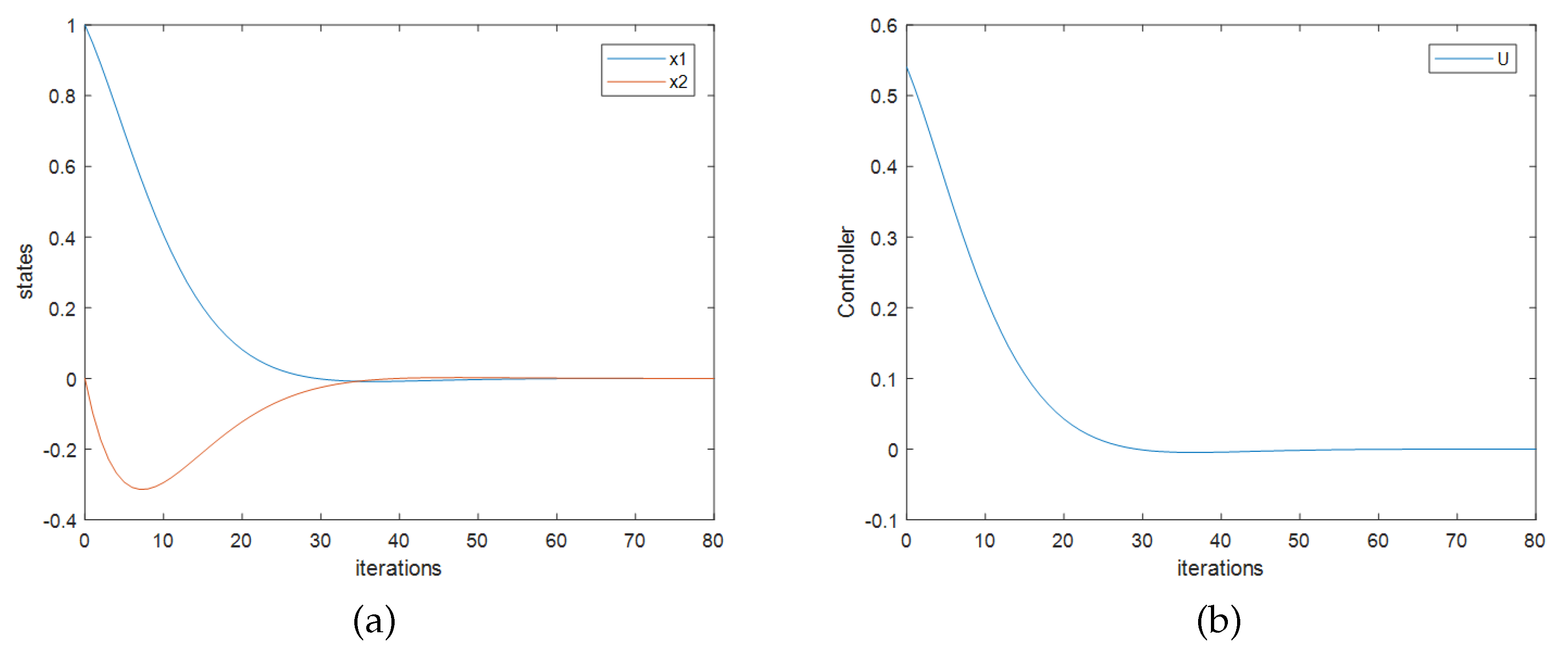
Figure 1 shows the closed-loop response and the control effort with the initial state of system
. In this figure, ordinates are values of states or control variables, and the horizontal ordinates are the computation times of the discrete-time system. The system is stable under the calculated feedback matrix, which means that the effective controller can be solved by the proposed method. There is a distinct different between the solved feedback matrix and the optimal theoretical value, the reason of that is the limitation of the information provided by the sampled data. With more data sets, the calculated feedback matrix will converge to the optimal theoretical value, as shown in example 2.
4.2. Example 2
Example 2: A DC motor discrete-time model described as two-order state equation is:
The weight matrices of performance criteria are: ,. The discount factor is .
To compare the optimal theoretical feedback matrix with the calculated one, a controller is designed by the traditional optimal control theory based on the mathematical model. So the matrices
and
are solved by Equation (
7):
,
. In addition, the solution of Equation (
5) is:
. The
can be calculated according to Equation (
8):
.
To get the feedback matrix by the existing Q-learning method, the initial feedback matrix is set as . To avoid the data deficiencies factor, the system has been sufficiently excited, and 1500 sets of date is sampled. According to Formula (11), the equation is obtained as following form:
To verify the above equation, the
calculated by Riccati equation and the
are substituted into it, and the two sides of the equation are equal. Therefore, the procedure of the calculation is proved correct. However, the
cannot be solved by Equation (
15), the analysis is as following. The eigenvalues of
is calculated as:
.
The rank of square matrix is 3, which means that the matrix is singular and noninvertible. Therefore the cannot be calculated via the least squares regression adopted by the existing Q-learning method.
While with the improved Q-learning method, the feedback matrix can be calculated as
. According to the ridge trace of
and
, the parameter
in Formula (14) is set as 0.01.
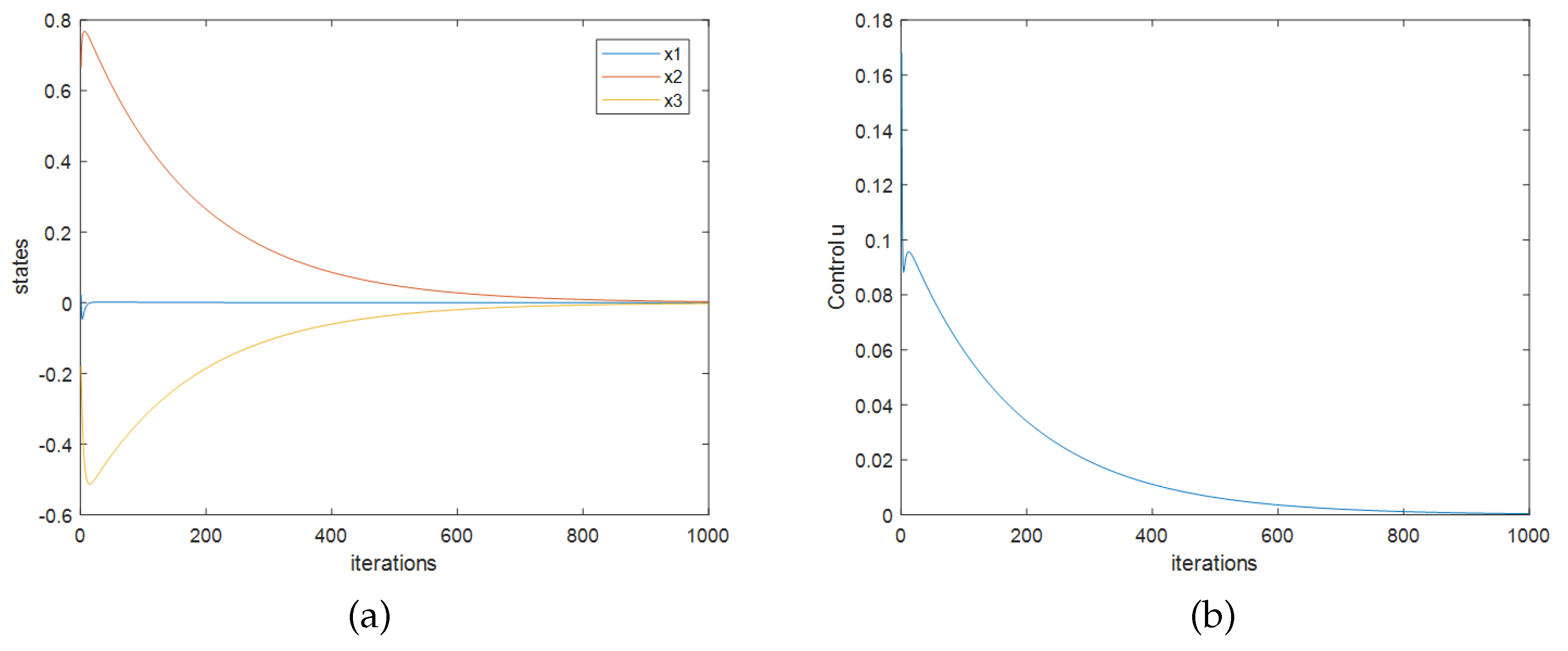
Figure 1 shows the closed-loop response and the control effects with the initial state of the system as
. Similar to example 1, the
Figure 1 shows that the system is closed-loop stable. Like in
Figure 2, ordinates of
Figure 1 are values of states or control variables, and the horizontal ordinates are the computation times of the discrete-time system. In
Figure 3 the ordinates and the horizontal ordinates are the same.
The initial feedback matrix is set as
, and the data acquisition process is the same as shown in example 1. The calculation process can be iterated repeatedly until
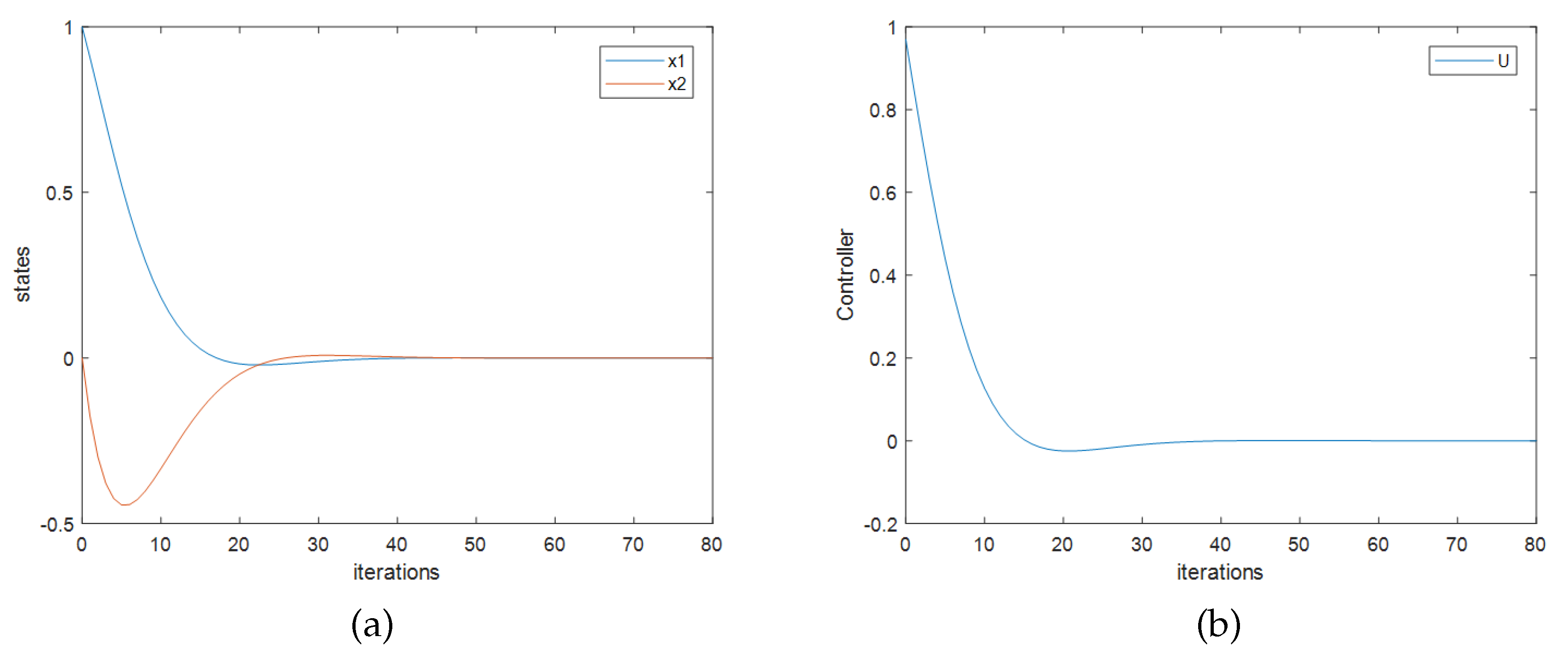
converges to a stable value or the system achieves satisfying performance. When the system obtains best performance, the calculated feedback matrix is
, and it is very close to the optimal theoretical value
. The simulation results are shown in
Figure 3. According to the simulation, for the linear discrete-time systems, the quadratic optimal controllers can be designed by online iterative calculation.
5. Further Analysis for Nonlinear Systems
The analysis and the simulation results both present that the quadratic optimal controllers for the linear discrete-time systems cannot be solved by Equation (
11). The corresponding analysis should be done to guide the design of Q-learning quadratic optimal controllers for nonlinear discrete-time systems and nonlinear continuous-time systems.
For nonlinear discrete-time systems described as
, the index of the optimized performance is defined as:
. And the Q function is defined as:
. Therefore, the Q function can be noted as:
where
is the vector of unknown parameters,
is sampled data set composed by state variables
and control variables
. The extreme condition derived from Formula (18) is shown as following form:
. The optimized solution of the above equation is noted as:
where
is the unknown parameters vector,
is the sampled data set composed by state vector
.
Theoretically, the controller can be solved by Formula (18) under the condition derived as Formula (19). While the elements of vector should be linear independent to solve adopting the least squares method. So the linear correlation of the vector should be discussed to ensure the calculation can be implemented correctly.
For nonlinear continuous-time systems described as:
, the index of the optimized performance is defined as:
. And the Q function is defined as following form.
Therefore, the Q function can be noted as:
where
is the unknown parameters vector,
is sampled data set composed by state variables and control variables. The extreme condition derived from Formula (20) is shown as the following form:
. The optimized solution of the above equation noted as:
where
is the unknown parameters vector,
is the sampled data set composed by state vector
.
Similar to nonlinear discrete-time systems, the quadratic optimal controllers for nonlinear continuous-time systems can be solved by Formula (20) under the extreme condition formed as Formula (21). And also the elements of vector should be linear independent to solve via the least square method. So the linear correlation of the vector should also be discussed to ensure the calculation can be implemented correctly.
In general, the problem about the multi-collinearity of data sets sampled from nonlinear systems no matter discrete-time or continuous-time needs to be discussed in further research to determine whether the existing Q-learning algorithm should be modified when it is used to deal with nonlinear systems. This will make positive significance for nonlinear systems control schemes such as microbial fuel cell systems [
35,
36]. The relative analysis and simulations will be developed in our further researching.
6. Conclusions
The design of optimal quadratic controllers for linear discrete-time systems based on Q-learning method is claimed as a kind of model-free method [
37,
38]. In this paper, both the theoretical analysis and the simulation results demonstrate that the existing design method of model-free controllers based on Q-learning algorithm ignores the linear independence of sampled data sets. For the linear discrete-time or continuous-time systems, the model-free quadratic optimal controllers cannot be established directly by the Q-learning method until the linear independence of data sets is guaranteed. The matrix
is inevitably column-related considering the quadratic optimal control law
. So other solution methods should be investigated besides the least squares method to solve parameters matrix
.
An improved Q-learning method based on ridge regression for linear discrete-time systems is proposed in this paper to deal with the multi-collinearity problem of the sampled data sets. Simulations show the effectiveness of the proposed method. There are deficiencies of the improved Q-learning method. First, the proposed method relies on the ridge trace of the linear correlation matrix, so the computation speed is limited. Second, the proposed method considers with neither disturbance nor saturation of controller. Further research will focus on solving these problems.
