Intelligent Colored Token Petri Nets for Modeling, Control, and Validation of Dynamic Changes in Reconfigurable Manufacturing Systems

Abstract

The invention of reconfigurable manufacturing systems (RMSs) has created a challenging problem: how to quickly and effectively modify an RMS to address dynamic changes in a manufacturing system, such as processing failures and rework, machine breakdowns, addition of new machines, addition of new products, removal of old machines, and changes in processing routes induced by the competitive global market. This paper proposes a new model, the intelligent colored token Petri net (ICTPN), to simulate dynamic changes or reconfigurations of a system. The main idea is that intelligent colored tokens denote part types that represent real-time knowledge about changes and status of a system. Thus, dynamic configurations of a system can be effectively modeled. The developed ICTPN can model dynamic changes of a system in a modular manner, resulting in the development of a very compact model. In addition, when configurations appear, only the changed colored token of the part type from the current model has to be modified. Based on the resultant ICTPN model, deadlock-free, conservative, and reversible behavioral properties, among others, are guaranteed. The developed ICTPN model was tested and validated using the GPenSIM tool and compared with existing methods from the literature.

1. Introduction

A manufacturing system (MS) is a conglomeration of robots, machine tools, fixtures, and buffers. Several types of products enter the MS at separate points in time. The system can process these parts based on a specified sequence of operations and resource sharing. In the competitive global market, MSs must handle unpredictable and rapid market changes. To cope with these dynamic changes, MSs need to execute quick changes in their software and hardware. Nevertheless, traditional manufacturing systems cannot successfully meet this requirement because they need large capital investments. To tackle these drawbacks in traditional manufacturing systems, reconfigurable manufacturing systems (RMSs) were developed [1,2,3]. RMSs are a new class of manufacturing systems and are subject to dynamic and random configurations in real time. These changes include processing failures and rework, machine breakdowns, addition of new machines, addition of new products, removal of old machines, and changes in processing routes.

To address the dynamic change problem in manufacturing systems, several approaches with Petri nets have been proposed. The study of Reference [4] presented a new higher-level deadlock control technique for the serial and parallel configuration of RMSs. RMSs have been used to replace traditional, large volume manufacturing systems, including dedicated production systems, providing more convertibility and flexibility. A rule-based matrix approach was developed and implemented in serial and parallel configurations. Higher-level deadlocks that are not prohibited by the existing approach were found through this type of application in the example RMS.

The study of Reference [5] introduced an improved net rewriting system (INRS)-based approach to automatically reconfigure an RMS supervisory controller based on Petri nets. Modifications to an RMS configuration were established into rules for rewriting that were then implemented in the original Petri net controller. First, the INRS was developed as the basis for reconfiguration. This can dynamically modify the structure of a Petri net model. Second, the study provided a triple representation of an RMS configuration and proposed an INRS-based approach to design a Petri net controller for an RMS. Finally, the article focused on providing an INRS-based approach for quick and automatic reconfiguration of this type of Petri net controller. In this approach, there is no verification or validation of the behavioral properties, i.e., reversibility, boundedness, and liveness for a reconfigured system.

A new Petri net model, called an intelligent token Petri net (ITPN), was presented by Reference [6]. In this model, tokens representing job types carry real-time knowledge about system changes and status, the same as intelligent cards in practice. An ITPN can model dynamic changes (adding new machines and products) in modular form, resulting in the development of a very compact model. If changes occur, only the changed part of the current model needs to be modified. To make an ITPN deadlock-free and reversible, a deadlock-free control policy was presented based on the ITPN model. In addition, when an ITPN is modified according to the system changes, the policy is still applicable to the modified model. Therefore, when an ITPN model is modified, the control policy need not be changed. However, the reconfiguration mechanism in ITPN needs to be further studied. Some of dynamic changes do not clearly define the modularity that may bring confusion to engineers in understanding and future redeveloping an RMS. Correctness of the system such as coherence of states before and after reconfiguration of the system is not considered. In addition, there is no mention of temporal constraints, which are of great significance in real-time systems.

The work of Reference [7] presented the reconfigurable finite-capacity Petri net (RFCPN) for the dynamic configuration of a flexible MS. An RFCPN is a Petri net extension that can be used for modeling, simulating, and validating simultaneous systems, which are subject to changes. Kahloul et al. [8] used reconfigurable object nets (RONs) to model, simulate, and analyze RMSs. The study proposed a formal approach to meet a new requirement (production of bricks used in slabs). A new extrusion machine (EMS) and a new cutting machine (CMS) were included in the configuration. The reconfiguration was defined as graph transformations, a simulation was performed using the RON tool, and software tools such as TINA-tool [9] and PIPE-tool [10] were used in the analysis.

The work of Reference [11] explored the principles of various methods and took the best practices from each one. Reconfiguration mechanisms were developed using Holonic and multiagent system approaches to enable the systematic detection of faults for a reconfigurable distributed production control system. The principle of service-oriented architecture was used to describe communication interfaces. Using Petri net models, hybrid top-down and bottom-up approaches were presented.

From the perspective of multiagent systems, a reconfigurable MS formal model (RMSFM) was developed in Reference [12], where two complementary formalisms (object-oriented Petri nets (ORPNs) and π-calculus) were used as formalisms. The ORPN was used to model both the initial structure and system behaviors of RMSs, while π-calculus was used to characterize the reconfiguration of RMSs. Petri Nets and π-calculus supporting tools were used to evaluate, check, and validate the RMSFM. π-calculus can analyze the reconfigurability mechanism and consistency of RMSs.

In the literature, several approaches with Petri nets were proposed to enhance dynamic change problems in MSs. However, most of them did not provide a reconfiguration mechanism or algorithm, could not ensure the PN’s behavioral properties (i.e., boundedness, liveliness, and reversibility), or could not guarantee the correctness, accuracy, or validity of the reconfiguration results. The aim of this paper is to propose an intelligent colored token Petri net (ICTPN) based on a knowledge base for a rapid and valid reconfiguration-based Petri net for RMS. The main idea is to use colored tokens denoting part types that represent real-time knowledge about the changes and status of a system. The knowledge is introduced in the transitions, and the transitions know where the colored tokens should be located based on their colors and knowledge. The proposed ICTPN will cope with dynamic changes such as processing failures and rework, machine breakdowns, addition of new machines, addition of new products, removal of old machines, and change processing routes. The proposed ICTPN will ensure that the PN’s behavioral properties, i.e., boundedness, liveliness, and reversibility, indicate that the modeled MS has finite states, is deadlock-free, and operates cyclically, respectively.

The proposed ICTPN can be implemented to Mass Customization Manufacturing (MCM) to solve its challenges, such as attempting to make the products available to customers in a timely manner, keeping high-quality production of a high variety of products, and achieving costs low to match those of standardized products. It can be introduced to the Lean Production (LP) concept, so that a company can apply an RMS to optimize the use of the part of resources for particular product families, and it can also decrease the waste induced by the part of an RMS’s idle resources. It can be applied for Agile Manufacturing (AM) to increase rapid changeover between products, rapid introduction to new products and unattended operation. It can be implemented to Flexible Manufacturing System (FMS) to increase the speed of responsiveness to a variety of markets and customers. In addition, increasing the scalability to the required products volume and convertibility to the existing systems, machines, robots, and controls to match new production specifications.

The rest of the paper is organized as follows. Section 2 describes the ICTPN and synthesis. Section 3 explains how to model dynamic configurations by ICTPN. Section 4 describes the qualitative and quantitative properties of ICTPNs. Finally, Section 5 presents the conclusions and future research.

2. Preliminary

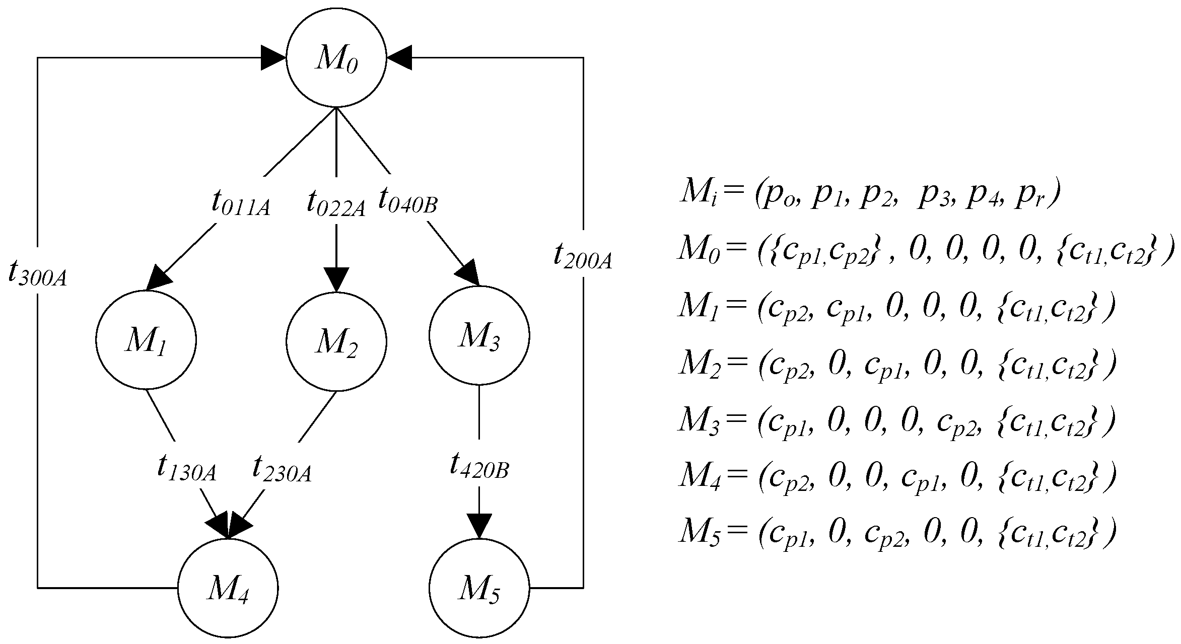
2.1. Definition of Intelligent Colored Token Petri Nets

Traditional Petri nets are popularly used to model, simulate, control, and analyze automated manufacturing systems (AMSs). Existing traditional Petri net studies assumed one or more of the following: (1) the system configuration is recognized and does not change throughout the operation, (2) there is no addition of new machines and no removal of old machines, and machine failures are not addressed, (3) rework is not required, and (4) products to be manufactured are identified, their process routes are specified, and the addition of new products is not applicable [13,14,15,16,17,18,19,20,21,22,23,24,25,26,27,28,29,30,31,32]. This means that traditional Petri net models do not undergo dynamic configurations, such as processing failures and rework, machine breakdowns, addition of new machines, addition of new products, removal of old machines, or change processing routes induced by the competitive global market. Therefore, an ICTPN based on a knowledge base for a rapid and valid reconfiguration-based Petri net for an RMS is proposed to deal with such dynamic changes. The main idea is that colored tokens denote part types that represent real-time knowledge about the changes and status of a system. Transitions know where the colored tokens should be located based on their colors and knowledge.

Definition 1.

Let N = (P_A ∪ {p_o} ∪ {p_r}, T, F, W, M_o, K) be a finite-capacity Petri net, where p_o is a common load/unload place that represents a part type to be processed in the system, p_r is a common transportation resource that represents transportation resources in the system, and P_A = {p₁, p₂, p₂,…, p_m} is a set of operation resources and P_A ∩ {p_r} = ∅. T is a finite non-empty set of transitions. F ⊆ (P × T) ∪ (T × P) is said to be a set of directed arcs of N that join the places to transitions or transitions to places, where P = P_A ∪ {p_o} ∪ {p_r}. W: (P × T) ∪ (T × P) → IN is a mapping that assigns an arc’s weight, where IN = {0, 1, 2, …}. M_o: P → IN is an initial marking of N. K: P → IN is a capacity function where K(p) represents the maximal number of tokens that place p can hold at a time.

Definition 2.

Let (N, M_o) be a finite-capacity Petri net with N = (P_A ∪ {p_o} ∪ {p_r}, T, F, W, M_o, K) and node a ∈ P_A ∪ {p_o} ∪ {p_r} ∪ T. Then, •a = {b ∈ P_A ∪ {p_o} ∪ {p_r} ∪ T | (b, a) ∈ F} is named the pre-set of node a, and a• = {b ∈ P_A ∪ {p_o} ∪ {p_r} ∪ T | (a, b) ∈ F} is named the post-set of node a.

Definition 3.

Let (N, M_o) be a colored finite-capacity Petri net with N = (P_A ∪ {p_o} ∪ {p_r}, T, F, W, M_o, K, SC, C_f, N_f, A_f, G_f, I_f), where P_A, p_o, p_r, T, F, W, M_o, and K are defined in Definition 1. SC is a color set that contains colors c_i and the operations on the colors. C_f is the color function that maps p_i ∈ P_C into colors c_i ∈SC. N_f is the node function that maps F into (P × T) ∪ (T × P). A_f is the arc function that maps each flow (arc) f ∈F into the term e. G_f is the guard function that maps each transition t_i ∈ T to a guard expression g that has a Boolean value. I_f is the initialization function that maps each place p_i ∈ P_C into an initialization expression.

Definition 4.

Let ICTPN be an intelligent colored token Petri net with N = (P_A ∪ {p_o} ∪ {p_r}, T, F, W, M_o, K, Ψ(p, c_pi, c_ti, d)), where

1. Given p ∈ P_A, M(p) is a marking of part type token with color as represented by M(p) = {c_pi\c_pi ∈ TC}, where TC represent the set of tokens with colors representing set of part types.

2. Given p = p_r, M(p) is a marking of transportation resource token with color as represented by M(p) = {c_ti\c_ti ∈ RC}, where RC represent the set of colors of transportation resources types.

3. Given p ∈ P_A ∪ {p_r}, c_pi ∈ TC, and c_ti ∈ RC, Ψ(p, c_pi, c_ti, d) is a knowledge function mapping tokens types c_pi and c_ti in place p at time d to a transition t, in which c_pi and c_ti can be used to enable t, as represented by Ψ(p, c_pi, c_ti, d)= {t\t ∈ T}.

Definition 5.

Let N = (P_A ∪ {p_o} ∪ {p_r}, T, F, W, M_o, K, Ψ(p, c_pi, c_ti, d)) be an ICTPN. An ICTPN with a marking is said to be acceptably marked if the following conditions are satisfied: (1) M_o(p_o) ≥ 1, (2) M_o(p_r) ≥ 1, and (3) M_o(p) = 0, ∀p ∈ P_A.

Definition 6.

Let ICTPN be an intelligent colored token Petri net with N = (P_A ∪ {p_o} ∪ {p_r}, T, F, W, M_o, K, Ψ(p, c_pi, c_ti, d)). A transition t ∈ T is enabled at marking M if the following conditions are satisfied: ∀p ∈ ^•t ∩ (P_A ∪ {p_r}), $\exists$c_pi ∈ M(^•t ∩ P_A),$\exists$c_ti ∈ M(^•t ∩ {p_r}), t ∈ Ψ(p, c_pi, c_ti, d), M(t^• ∩ P_A) − {c_pi} < K(t^• ∩ P_A), and M(t^• ∩ {p_r}) − {c_pi} < K(t^• ∩ {p_r}).

Definition 7.

Let ICTPN be an intelligent colored token Petri net with N = (P_A ∪ {p_o} ∪ {p_r}, T, F, W, M_o, K, Ψ(p, c_pi, c_ti, d)). N has a self-loop if for all a, b ∈ P_A ∪ {p_o} ∪ {p_r} ∪ T, W(a, b) > 0 implies W(b, a) > 0.

Definition 8.

Let ICTPN be an intelligent colored token Petri net with N = (P_A ∪ {p_o} ∪ {p_r}, T, F, W, M_o, K, Ψ(p, c_pi, c_ti, d)). N is self-loop free if for all a, b ∈ P_A ∪ {p_o} ∪ {p_r} ∪ T, W(a, b) > 0 implies W(b, a) = 0.

Definition 9.

Let ICTPN be an intelligent colored token Petri net with N = (P_A ∪ {p_o} ∪ {p_r}, T, F, M_o, K, Ψ(p, c_pi, c_ti, d)). A transition t ∈ T that is enabled at marking M by c_pi and c_ti may fire. The marking of the ICTPN can be changed from M to M′ as follows:

$$M\prime (p)=\left[\begin{array}{ll}M\left(p\right)-\left\{c_{pi}\right\}& \mathrm{if} p{\in }^{•}t\cap P_A\\ M\left(p\right)+\left\{c_{pi}\right\}& \mathrm{if} p\in t^{•}\cap P_A\\ M\left(p\right)-\left\{c_{ti}\right\}& \mathrm{if} p{\in }^{•}t\cap \left\{p_r\right\}\\ M\left(p\right)-\left\{c_{ti}\right\}& \mathrm{if} p\in t^{•}\cap \left\{p_r\right\}\\ M\left(p\right)& \mathrm{Otherwise}\end{array}\right]$$

Definition 10.

Let ICTPN be an intelligent colored token Petri net with N = (P_A ∪ {p_o} ∪ {p_r}, T, F, W, M_o, K, Ψ(p, c_pi, c_ti, d)). N is known as an ordinary net if ∀(p, t) ∈ F, W(p, t) = 1, where N = (P, T, F). N is named a weighted net if there is an arc between x and y such that W(x, y) >1.

Definition 11.

Let ICTPN be an intelligent colored token Petri net with N = (P_A ∪ {p_o} ∪ {p_r}, T, F, W, M_o, K, Ψ(p, c_pi, c_ti, d)). The set of markings that are reachable from M in N is named the set of reachability of the Petri net model (N, M), denoted by R (N, M). A transition t ∈ T is live if for all M ∈ R(N, M), there exists a reachable marking M′ ∈ R(N, M) such that M′[$t\rangle$holds. A net system (N, M₀) is dead at M_o if there does not exist t ∈ T such that M_o[$t\rangle$holds.

Definition 12.

Let ICTPN be an intelligent colored token Petri net with N = (P_A ∪ {p_o} ∪ {p_r}, T, F, W, M_o, K, Ψ(p, c_pi, c_ti, d)). A marking M_o is a reversible if, for each marking M′ ∈ R(N, M_o), M_o is reachable from M′.

Definition 13.

Let ICTPN be an intelligent colored token Petri net with N = (P_A ∪ {p_o} ∪ {p_r}, T, F, W, M_o, K, Ψ(p, c_pi, c_ti, d)). A marking M′ is a coverable if there exists a marking M″ ∈ R(N, M_o) such that M″(p) ≥ M′(p) for each p in the N.

Definition 14.

Let ICTPN be an intelligent colored token Petri net with N = (P_A ∪ {p_o} ∪ {p_r}, T, F, W, M_o, K, Ψ(p, c_pi, c_ti, d)). [N] is said to be the incidence matrix of net N, where [N] is an integer matrix that consists of |T| columns and |P| rows with [N](p, t) = W(t, p) −W(p, t).

Definition 15.

Let ICTPN be an intelligent colored token Petri nets with N = (P_A ∪ {p_o} ∪ {p_r}, T, F, W, M_o, K, Ψ(p, c_pi, c_ti, d)). A marking M′ is said to be reachable from M if there exist a finite transition sequence δ = t₁ t₂ t₃ … t_n that can be fired, and markings M₁, M₂, M₃, …, and M_n−1 such that M[$t_1\rangle$M₁[$t_2\rangle$M ₂[$t_3\rangle$M ₂ … M_n−1[$t_n\rangle$M′, denoted as M[$\delta \rangle$M′, satisfies the state equation M′ = M + [N]$\overrightarrow{\delta }$, where$\overrightarrow{\delta }$: T → IN maps t in T to the number of appearances of t in δ and is called a Parikh vector or a firing count vector.

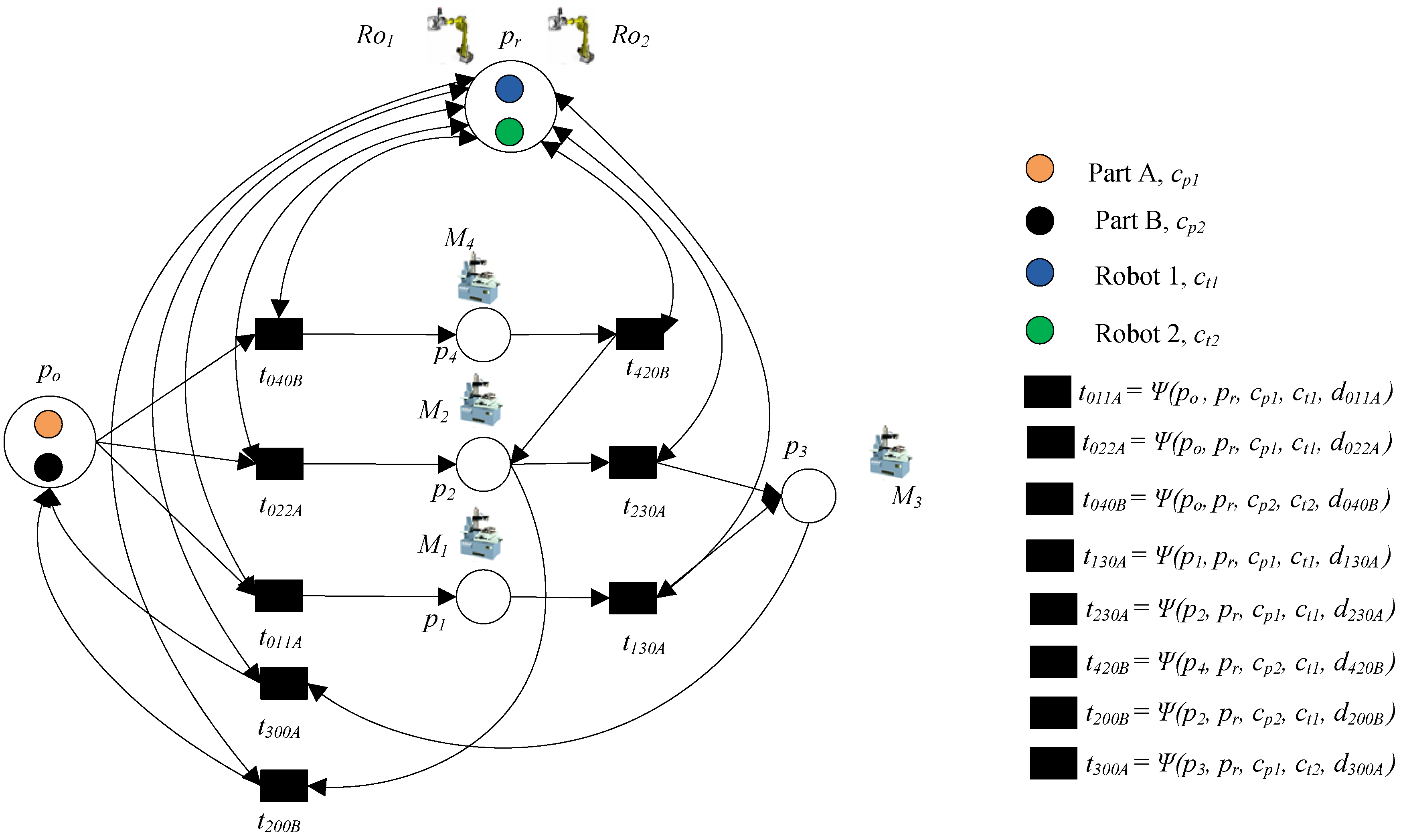
2.2. Design of Intelligent Colored Token Petri Nets

In AMS, let OR = {OR₁, OR₂, OR₃, …, OR_n} be all possible routes and should be manufactured in a system for all types of parts PT, where OR_i is R_o → R_i1 → R_i2 → ……→ R_iFi → R_o, n, F_i are large integer numbers, R_o denotes a load/unload station of the system with infinite capacity, and R_i(i ≠ 0) may be a buffer or machine, which is named an operation resource. An operation route starts from R_o and ends at R_o. For each part, if there exists more than one operation route such that R_i → R_{j(i ≠ j)}, it is said that there is a path from R_i to R_j. When a part transfers from R_i to R_j, namely it is transported by a material handling device, such as an AGV or robot that is named a transportation resource.

In Definition 4, Ψ(p, c_pi, c_ti, d) knows where colored tokens c_pi and c_ti should go based on their colors and knowledge and knows the system configuration and the state of the tokens themselves. Because of this, c_pi and c_ti are named intelligent colored tokens. An approach can be used to synthesize the ICTPN irrespective of how complicated the system operation routes are.

According to part routing information and transportation requirements, the modeling of operation and transportation resources is stated as follows:

Algorithm 1:Modeling operation and transportation resources

Initialization:Build a common load/unload place po and common transportation resource place pr, π = {Ro}, c = 0, j=0, and h = 0.

for (1, n, i++), choose ORi ∈ OR, do

while j < Fi, do

j = j + 1

if Rij ∈ π, then

Build the place that corresponds to Ri(j-1), which is pa

Build the place that corresponds to Rij, which is pb

Build a transition tabhi and knowledge function Ψ(pa, cpi, dabhi)

Build an arc from pa to tabhi and an arc from tabhi to pb

if tabhi needs common place pr to transport part i from pa to pb, then

Update a knowledge function to Ψ(pa, pr, cpi, cti, dabhi)

Insert an arc from pr to tabhi and an arc from tabhi to pr.

end if

else

π = π ∪ {Rij}

c = c + 1

Build a place and name it pc

Identify the place that corresponds to Ri(j-1), which is pa

Build a transition tachi and knowledge function Ψ(pa, cpi, dachi)

Build an arc from pa to tachi and an arc from tachi to pc

if tachi needs common place pr to transport part i from pa to pc, then

Update a knowledge function to Ψ(pa, pr, cpi, cti, dachi)

Insert an arc from pr to tachi and an arc from tachi to pr.

end if

end if

end while

Identify the place that corresponds to RiFi, which is pa

Build a transition ta0hi and knowledge function Ψ(pa, cpi, da0hi)

Build an arc from pa to ta0hi and an arc from ta0hi to po

if ta0hi needs common place pr to transport part i from pa to po, then

Update a knowledge function to Ψ(pa, pr, cpi, cti, da0hi)

Insert an arc from pr to ta0hi and an arc from ta0hi to pr.

end if

end for

/ * Define the initial marking of the system */

Place tokens with colors into common load/unload place po such that Mo(po) = {cp1, cp2, cp3, … cpn} ⊂ TC, where cpi ∈ TC, i∈ PT, which denotes that a part type i to be processed in the system. Place tokens with colors into common transportation resource place pr such that Mo(pr) = {ct1, ct2, ct3, … ctk} ⊂ RC, where cti ∈ RC, which denotes a transportation resource in the system. Mo(p) = 0, for all p ∈ PA.

Output: The ICTPN model

To demonstrate the synthesis of an ICTPN, consider an AMS example, shown in Figure 1a. The AMS Petri net model is given in Chen et al. [33], Piroddi et al. [34], Chen and Li [35], Chen et al. [36], and Kaid et al. [37]. The system is composed of four machines (M₁, M₂, M₃ and M₄; each machine can process one part at a time) and two robots (Ro₁ and Ro₂; each robot can hold a part at a time). There is a loading/unloading buffer. Two part-types, A and B, are considered to be processed in the system. The operations sequences of these two part-types are shown in Figure 1b. The operation and transportation resources model is shown in Figure 2, for operation resources, p₁, p₂, p₃, and p₄ model M₁, M₂, M₃, and M₄, respectively. The process route of Part A is constructed by p_o → t_011A → p₁ → t_130A → p₃ → t_300A → p₀, or p_o → t_022A → p₂ → t_230A → p₃ → t_300A → p₀. The process route of Part B is constructed by p_o → t_040B → p₄ → t_420B → p₂ → t_200B → p₀, for transportation resources, common place p_r models Ro₁ and Ro₂.

To model the transportation operations of part types, transition t_011A denotes loading part A to p₁ and transition t_022A denotes loading part A to p₂, where Ro₁ is needed. Transition t_300A denotes unloading part A from p₃, where Ro₂ is needed. Transitions t_040B denotes loading part B to p₄, where Ro₂ is needed, and transition t_200B denotes unloading part B from p₂, where Ro₁ is needed. These operations can be done by developed common place p_r. Thus, common place p_r and arcs (p_r, t_011A), (t_011A, p_r), (p_r, t_022A), (t_022A, p_r), (p_r, t_300A), (t_300A, p_r), (p_r, t_040B), (t_040B, p_r), (p_r, t_200B), and (t_200B, p_r) are inserted into the model. Transporting part A between p₁ and p₃ (Ro₁ is needed) or p₂ and p₃ (Ro₁ is needed) is represented by transitions t_130A or t_230A, respectively. Transporting part B between p₄ and p₂ (Ro₁ is needed) is represented by transitions t_420B. Thus, common place p_r and arcs (p_r, t_130A), (t_130A, p_r), (p_r, t_230A), (t_230A, p_r), (p_r, t_420B), and (t_420B, p_r) are inserted into the model.

Note that in ICTPN, transition t has one input place from p ∈ P_A, one input place from p_r, one output place to p ∈ P_A, and one output place to p_r. Next, to define the initial marking of the system, place tokens with colors into place p_o such that M_o(p_o) = {c_p1, c_p2}, where c_p1 and c_p2 denote a part type A and part type B, respectively. Place tokens with colors into place p_r such that M_o(p_r) = {c_t1, c_t2}, where c_t1 and c_t2 denote transportation resources in the system Ro₁ and Ro₂, respectively.

Consider the ICTPN model shown in Figure 2. If the condition given in Definition 6 is satisfied, then we can say that t is enabled by c_pi and c_ti. By Definition 9, the marking of the ICTPN can be changed as follows. When transition t_011A (Ψ(p_o, p_r, c_p1, c_t1, d_011A)) fires for duration d_011A, it selects only one token with color c_p1 from input place p_o and one token with color c_t1 from input place p_r. If t_011A fires, then it transfers only one token with color c_p1 to output place p₁ and one token with color c_t1 to output place p_r. When transition t_022A (Ψ(p_o, p_r, c_p1, c_t1, d_022A)) fires for duration d_022A, then it selects only one token with color c_p1 from input place p_o and one token with color c_t1 from input place p_r. If t_022A fires, it transfers only one token with color c_p1 to output place p₂ and one token with color c_t1 to output place p_r. When transition t_040B (Ψ(p_o, p_r, c_p2, c_t2, d_040B)) fires for duration d_040B, then it selects only one token with color c_p2 from input place p_o and one token with color c_t2 from input place p_r. If t_040B fires, it transfers only one token with color c_p2 to output place p₄ and one token with color c_t2 to output place p_r. In addition, if transition t_130A (Ψ(p₁, p_r, c_p1, c_t1, d_130A)) fires for duration d_130A, it selects only one token with color c_p1 from input place p₁ and one token with color c_t1 from input place p_r. If t_130A fires, it transfers only one token with color c_p1 to output place p₃ and one token with color c_t1 to output place p_r. Moreover, when transition t_230A (Ψ(p₂, p_r, c_p1, c_t1, d_230A)) fires for duration d_230A, it selects only one token with color c_p1 from input place p₂ and one token with color c_t1 from input place p_r. If t_230A fired, it transfers only one token with color c_p1 to output place p₃ and one token with color c_t1 to output place p_r. If transition t_420B (Ψ(p₄, p_r, c_p2, c_t1, d_420B)) fires for duration d_420B, it selects only one token with color c_p2 from input place p₄ and one token with color c_t1 from input place p_r. If t_420B fires, it transfers only one token with color c_p2 to output place p₂ and one token with color c_t1 to output place p_r. Then, when transition t_200B (Ψ(p₂, p_r, c_p2, c_t1, d_200B)) fires for duration d_200B, it selects only one token with color c_p2 from input place p₂ and one token with color c_t1 from input place p_r. If t_200B fires, it transfers only one token with color c_p2 to output place p_o and one token with color c_t1 to output place p_r. Finally, if transition t_300A (Ψ(p₃, p_r, c_p1, c_t2, d_300A)) fires for duration d_300A, it selects only one token with color c_p1 from input place p₃ and one token with color c_t2 from input place p_r. If t_300A fires, it transfers only one token with color c_p1 to output place p_o and one token with color c_t2 to output place p_r.

3. RMS Configuration Changes Modeling Based on ICTPN

3.1. Machine Breakdowns

In an automated manufacturing system, the breakdown of its machines is usually caused by quality out-of-control signals, missing or defective part programs or tools, damaged tools, or the failure of sensing and actuating systems. For example, if a machine breakdown is detected, the operations that use the broken machine need to be performed by another machine. In this case, some processing routes are changed, which implies a modification to the structure of its Petri net model. Reconsider the ICTPN model shown in Figure 2. There are four machine tools, denoted by p₁, p₂, p₃, and p₄. Assume that p₁ is down and p₄ will perform the operations that were previously performed by itself and performed by p₁. Therefore, the structure of the ICTPN model is changed and will be re-designed such that the system with the removal of resource p₁ can operate continuously without stoppage. Hence, to model the reconfigured system, consider the following procedures:

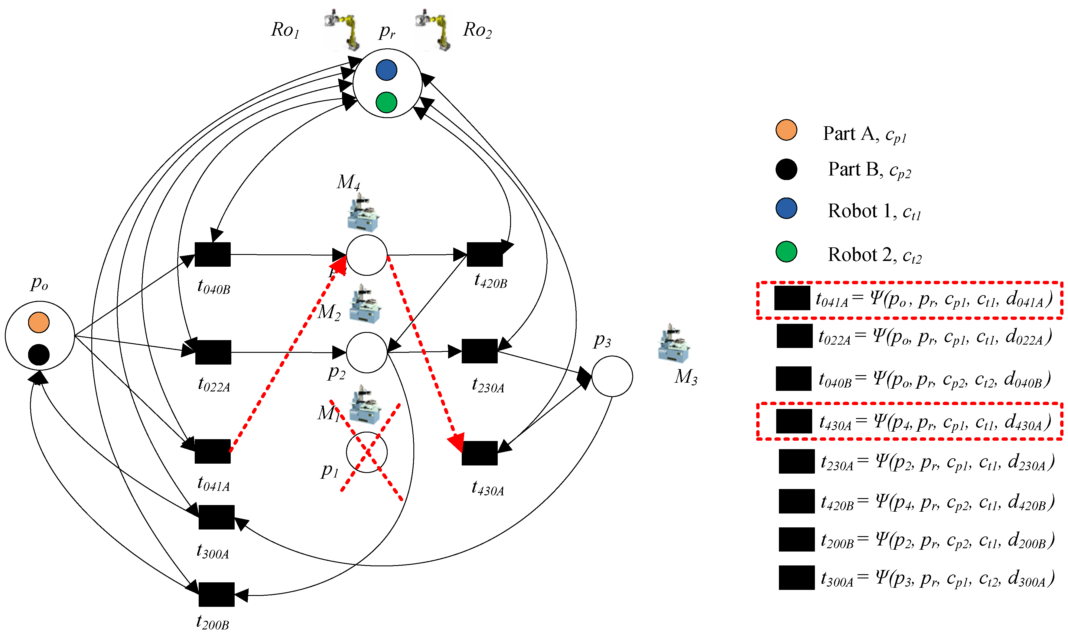
• Step 1: Disable the transitions connected to the place corresponding to the breakdown machine and remove or disable this place p₁.
• Step 2: Change the names of transitions based on new machine p₄
• Step 3: Change the operation route from p_o → t_011A → p₁ → t_130A → p₃ → t_300A → p₀ to p_o → t_041A → p₄ → t_430A → p₃ → t_300A → p₀.
• Step 4: Connect the transitions to the new machine p₄.
• Step 5: Change the names of the knowledge function of transitions based on new machine p₄.

t_041A = Ψ(p_o, p_r, c_p1, c_t1, d_041A)

t_430A = Ψ(p₄, p_r, c_p1, c_t1, d_430A )

An ICTPN for the reconfigured system by machine breakdowns is shown in Figure 3.

3.2. Addition of New Product

The second automated manufacturing system reconfiguration involves the addition of a new product. When a new product is added to a system, it means that a new route is added, which implies a modification to the structure of its Petri net model. To model the newly added route by using the ICTPN synthesis procedure, reconsider the ICTPN model shown in Figure 2. Assume that a new product part C is added. It processing route is constructed by load/unload station → M₄ → M₃ → load/unload station. To transport part C between the load/unload station and M₄, Ro₂ is needed, and to transport part C between M₄ and M₃, Ro₁ is needed. Hence, to model the reconfigured system, consider the following procedures:

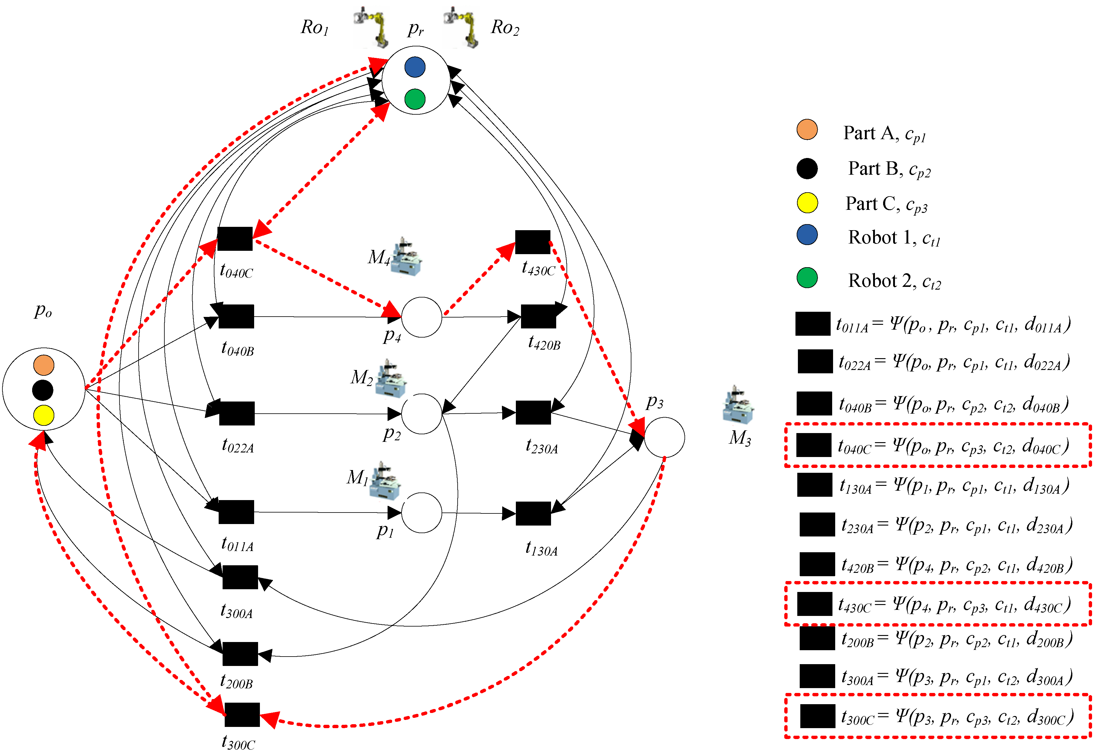
• Step 1: Add a new operation route from p_o → t_040C → p₄→ t_430C → p₃ → t_300C → p₀.
• Step 2: Add the transportation operation of part C. Transition t_040C denotes loading part C to p₄, and Ro₂ is needed; t_430C denotes transporting part C to p₃ and Ro₁ is needed. Transition t_300C denotes unloading part C from p₃ and Ro₂ is needed. These operations can be done by common place p_r.
• Step 3: Add the knowledge function of transitions based on a new operation route.

t_040C = Ψ(p_o, p_r, c_p3, c_t2, d_040C)

t_430C = Ψ(p₄, p_r, c_p3, c_t1, d_430C)

t_300C = Ψ(p₃, p_r, c_p3, c_t2, d_300C).

• Step 4: Place the token with color c_p3 into place p_o, which denotes a part C that will be processed in the system.

An ICTPN for the reconfigured system by the addition of a new product is shown in Figure 4.

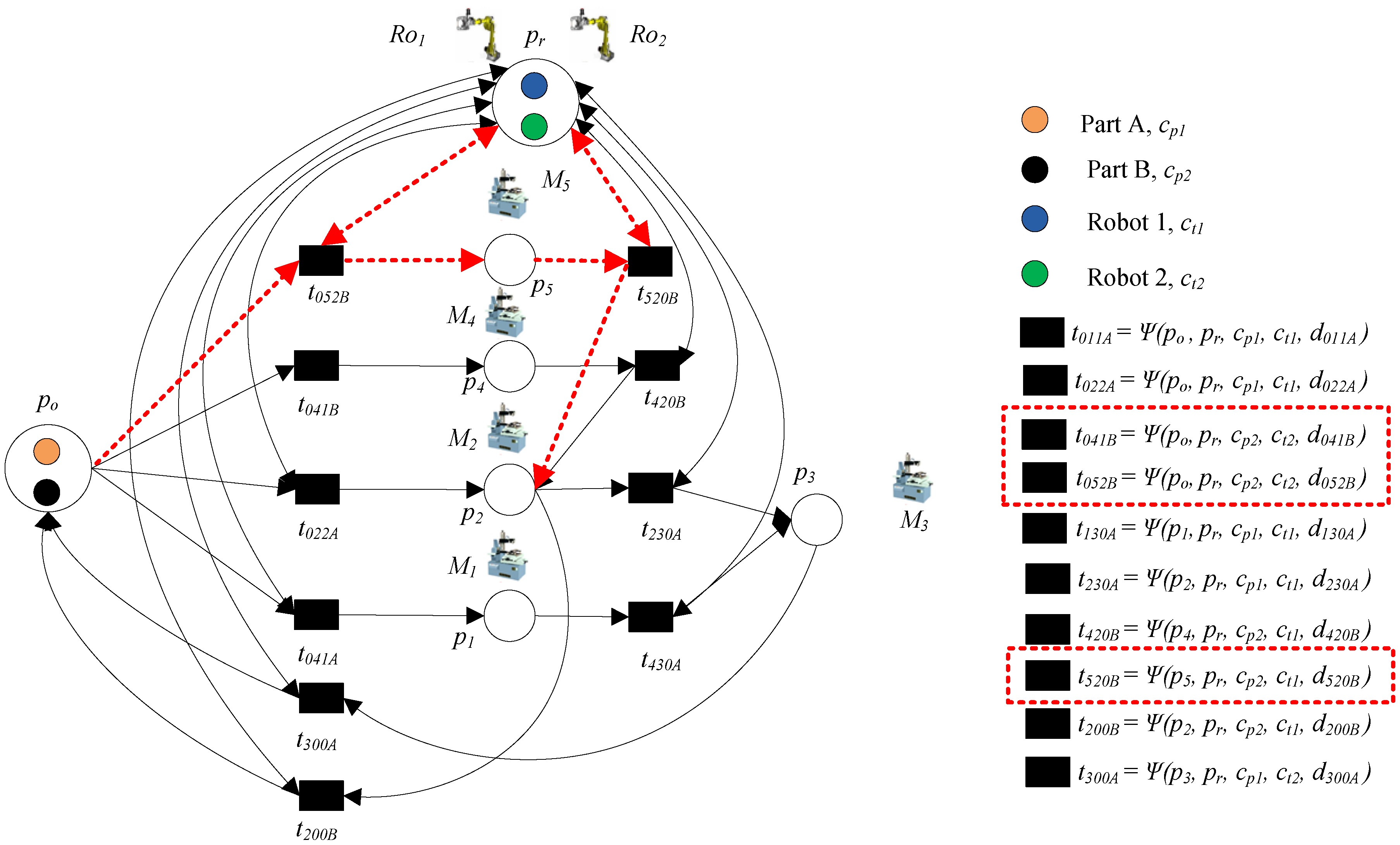
3.3. Addition of New Machine

The third system reconfiguration includes the addition of a new machine. In this case, a new machine is added to the system. Operations for new or used parts are conducted by the newly added machine. Moreover, new job processing routes can be generated, which implies the modification of the structure of the Petri net model. To model the newly added machine by using the ICTPN synthesis procedure, new places and transitions can be added based on the original ICTPN.

Consider the ICTPN model shown in Figure 2. Assume that a new machine M₅ is added to process part B. The processing route of part B is constructed by load/unload station → M₄ or M₅ → M₂→ load/unload station. To transport part B between the load/unload station and M₄ or M₅, Ro₂ is needed, and to transport part B between M₄ or M₅ and M₂, Ro₁ is needed. Hence, to model the reconfigured system, consider the following procedures:

• Step 1: Add process routes of part B as route 1: p_o → t_041B → p₄ → t_420B → p₂ → t_200B → p₀, or route 2: p_o → t_052B → p₅ → t_520B → p₂ → t_200B → p₀
• Step 2: Add the transportation operation of part B. Transitions t_041B and t_052B denote loading part B to p₄ and p₅, respectively, where Ro₂ is needed; t_420B and t_520B denote transporting part B to p₂, where Ro₁ is needed; these operations can be done by common place p_r.
• Step 3: Add the knowledge function of transitions based on a new machine

t_041B = Ψ(p_o, p_r, c_p2, c_t2, d_041B )

t_052B = Ψ(p_o, p_r, c_p2, c_t2, d_052B )

t_520B = Ψ(p₄, p_r, c_p3, c_t1, d_520B )

An ICTPN for the reconfigured system with the addition of a new machine is shown in Figure 5.

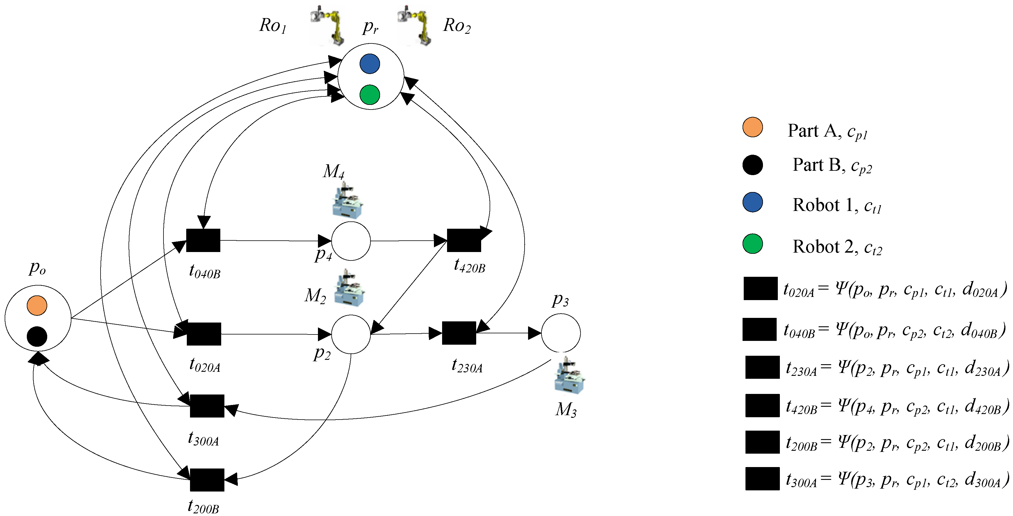
3.4. Removal of Old Machine

The fourth system reconfiguration includes the removal of an old machine. This indicates that the operations that use the removed machine need to be performed by another machine. Thus, some processing routes are changed, which implies a modification to the structure of its Petri net model. Reconsider the ICTPN model shown in Figure 2. Assume that machine 1 p₁ is removed from the system, and p₂ will perform the operations that are previously performed by itself and performed by p₁. Therefore, the structure of the ICTPN model is changed and will be re-designed, such that the system with the removal of machine p₁ can operate continuously without stoppage. Hence, to model the reconfigured system, consider the following procedures:

• Step 1: Delete all the transitions connected to the place corresponding to the removed machine p₁ and remove this place p₁.
• Step 2: One operation route will be considered, which is p_o → t_020A → p₂ → t_230A → p₃ → t_300A → p₀.
• Step 3: Delete the old knowledge function of transitions based on removed machine p₁.

t_011A = Ψ(p_o, p_r, c_p1, c_t1, d_011A )

t_130A = Ψ(p₄, p_r, c_p1, c_t1, d_130A )

An ICTPN for the reconfigured system by removal of an old machine is shown in Figure 6.

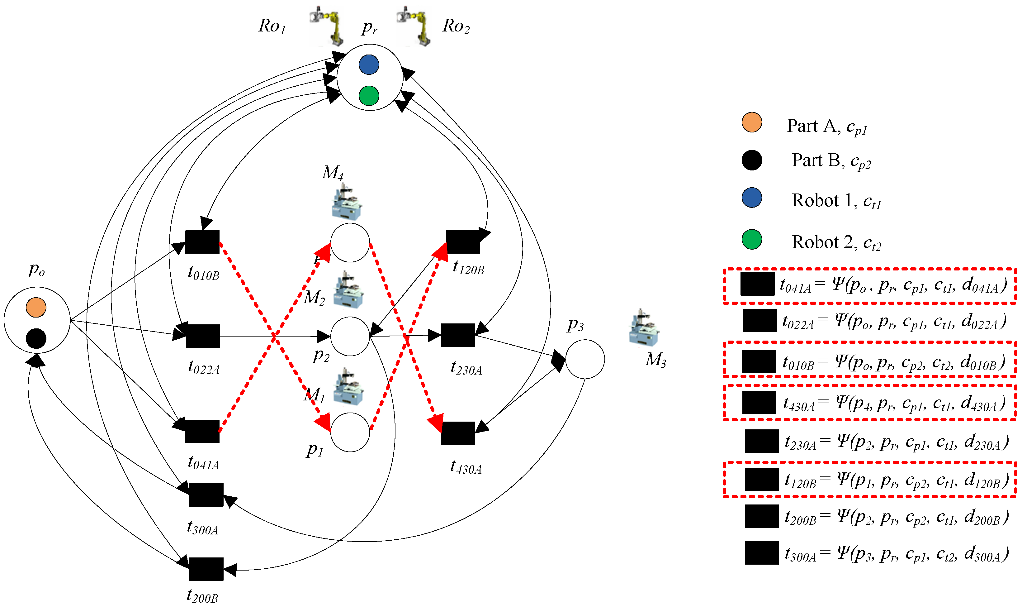
3.5. Change Processing Routes

The fifth system reconfiguration includes the change of processing routes. In this case, processing routes of parts are changed in the system, which implies a modification of the structure of its Petri net model. Reconsidering the ICTPN model shown in Figure 2, assume that the processing route of part A changes from p_o → p₁→ p₃ → p₀, or p_o → p₂ → p₃ → p₀ to p_o → p₄→ p₃ → p₀, or p_o → p₂ → p₃ → p₀, and the processing route of part B changes from p_o→ p₄ → p₂ → p₀ to p_o→ p₁ → p₂ → p₀. Therefore, the structure of the ICTPN model is changed and redesigned, such that the system works with changed processing routes. Hence, to model the reconfigured system, consider the following procedures:

• Step 1: Change the names of transitions based on processing routes.
• Step 2: Change the operation route of part A from p_o → t_011A → p₁ → t_130A → p₃ → t_300A → p₀ to p_o → t_041A → p₄ → t_430A → p₃ → t_300A → p₀.
• Step 3: Change the operation route of part A from p_o → t_040B → p₄ → t_420B → p₂ → t_200B → p₀ to p_o → t_010B → p₁ → t_120B → p₂ → t_200B → p₀.
• Step 4: Update the knowledge function of transitions based on removed machine p_1.

t_041A = Ψ(p_o, p_r, c_p1, c_t1, d_041A )

t_430A = Ψ(p₄, p_r, c_p1, c_t1, d_430A )

t_010B = Ψ(p_o, p_r, c_p1, c_t2, d_010B )

t_120B = Ψ(p₁, p_r, c_p2, c_t1, d_120B )

An ICTPN for the reconfigured system by the removal of an old machine is shown in Figure 7.

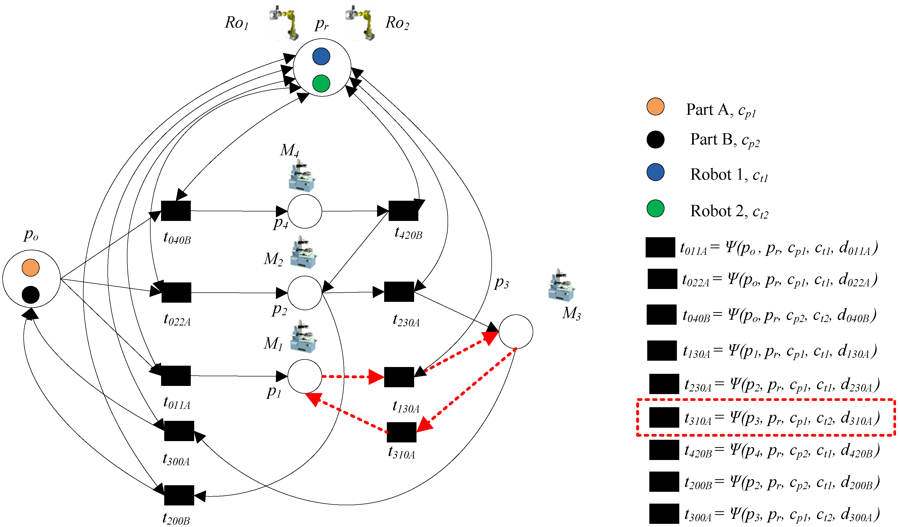
3.6. Rework

The sixth system reconfiguration includes rework. In this case, a part may be inspected when some of its operations are finished. If the reconfiguration is performed properly, then the system will continue based on an original route. Otherwise, rework is required. By using an ICTPN, the manufacturing operations of the reworked part can be easily and exactly modeled by considering rework operations as alternative routes. Reconsider the ICTPN model shown in Figure 2. Assume that M₃ is an inspection machine and that part A is processed in M₁ or M₂. Then, part A is transported to an inspection machine M₃ by Robot 1 to determine if there are defects in part A. If part A performs properly, then it will depart the system by Robot 2. Otherwise, if part A has defects, rework is required, and part A is removed and transported to M₁ by Robot 2. Thus, part A has four possible routes:

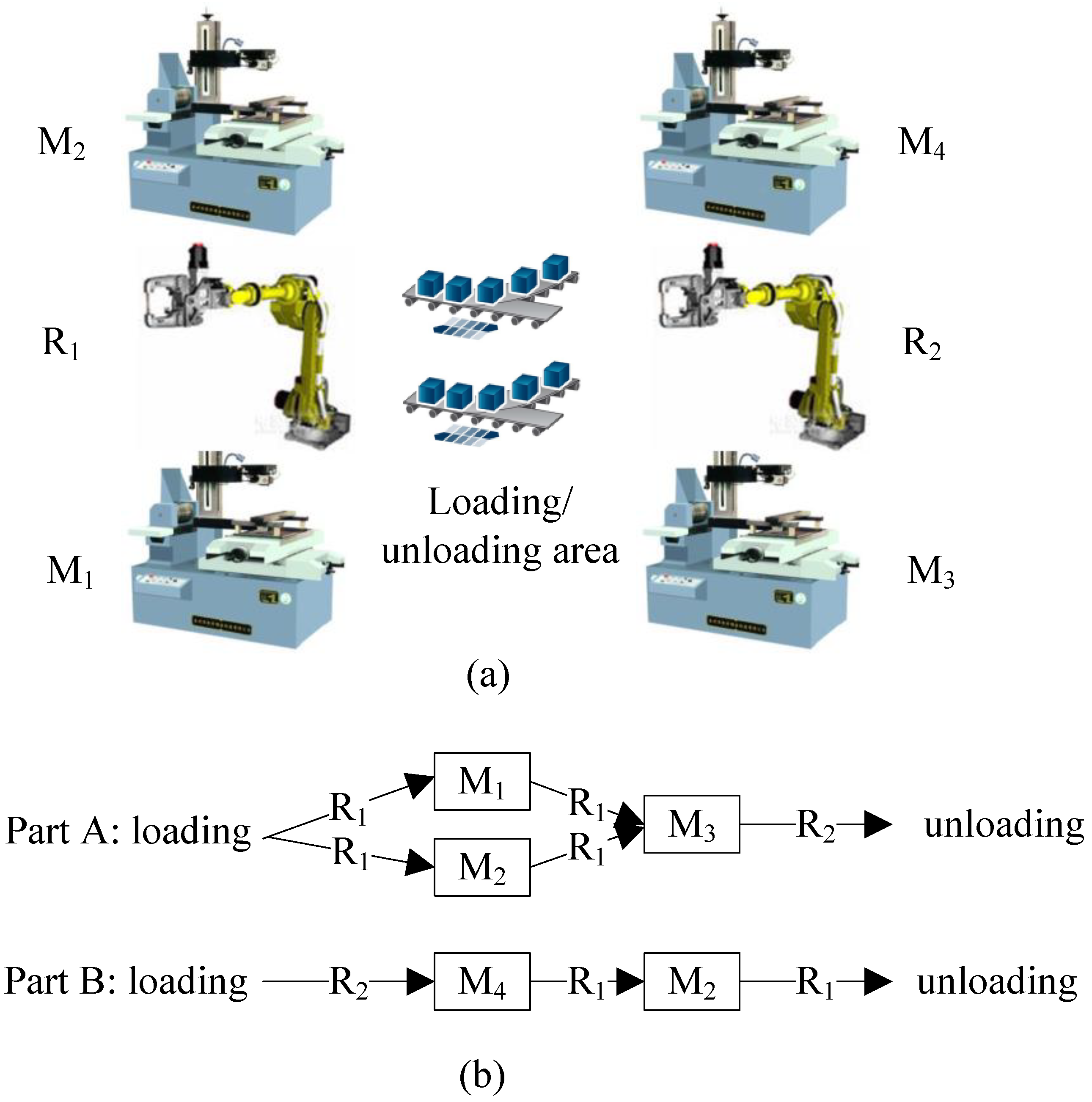
• Load–unload station → M₁ → inspection machine M₃ → load–unload station,
• Load–unload station → M₂ → inspection machine M₃ → load–unload station,
• Load–unload station → M₁ → inspection machine M₃ → M₁ → inspection machine M₃ → load–unload station, or
• Load–unload station → M₂→ inspection machine M₃ → M₁ → inspection machine M₃ → load–unload station.

Therefore, to model two routes by using the ICTPN synthesis procedure, a new transition can be added based on the original ICTPN. Hence, to model the reconfigured system, consider the following procedures:

• Step 1: Add the process routes of part B as route 1: p_o → t_011A → p₁ → t_130A → p₃ → t_300A → p₀, route 2: p_o → t_022A → p₂ → t_230A → p₃ → t_300A → p₀, route 3: p_o → t_011A → p₁ → t_130A → p₃ → t_310A → p₁ → t_130A → p₃ → t_300A → p₀, or route 4: p_o → t_022A → p₁ → t_230A → p₃ → t_310A → p₁ → t_130A → p₃ → t_300A → p₀.
• Step 2: Add the knowledge function of transition based on rework:

T_310A = Ψ(p₃, p_r, c_p1, c_t2, d_310B )

An ICTPN for the reconfigured system by rework is shown in Figure 8.

4. Qualitative and Quantitative Study of ICTPN

4.1. Deadlock

A deadlock is a situation in which each process in a set of processes enters a waiting state because a requested resource is being held by another waiting process, which in turn is waiting for another resource. Thus, deadlocks should be avoided or prevented.

Theorem 1.

The ICTPN is an intelligent colored token Petri net with N = (P_A ∪ {p_o} ∪ {p_r}, T, F, W, M_o, K, and Ψ(p, c_pi, c_ti, d)), and is deadlock-free (live).

Proof. 

There is a need to prove that all transitions T in the ICTPN are live. It does not matter how the system changes. For all t ∈ T, if ∀p_i ∈ ^•t and M_C(p_i) > 0, then t can fire in any case because it is uncontrollable. □

To demonstrate the liveness of an ICTPN, consider the ICTPN model shown in Figure 2. Figure 9 shows the reachability graph of the ICTPN, and the system is live.

4.2. Conservativeness

Conservativeness is one of the main characteristics of ICTPN, where a transition, t, has one input place and one output place in p_r, i.e., |^•t ∩ {p_r}| = |t^• ∩ {p_r}|=1, and one input place and one output place in P_A, i.e., |^•t ∩ P_A | = |t^• ∩ P_A | = 1. Therefore, in the incidence matrix D for an ICTPN, there is one –1 and one 1 in each row. Thus, if y = (1, 1, …, 1)^T, Dy = 0 must hold. For instance, reconsider the ICTPN model shown in Figure 2. We have P = (p_o, p₁, p₂, p₃, p₄, p_r) and T= (t_011A, t_022A, t_040B, t_130A, t_230A, t_420B, t_200B, t_300A). The incidence matrix D of ICTPN model shown in Figure 2 is stated as follows:

D =	−1	0	1	0	0	0
	−1	0	0	1	0	0
	−1	0	0	0	0	1
	0	0	−1	0	1	0
	0	0	0	−1	1	0
	0	0	0	1	0	−1
	1	0	0	−1	0	0
	1	0	0	0	−1	0

Thus, Dy = 0 is satisfied with y = (1, 1, 1, 1, 1, 1)^T

−1	0	1	0	0	0
−1	0	0	1	0	0		1		0
−1	0	0	0	0	1		1		0
0	0	−1	0	1	0		1		0
0	0	0	−1	1	0	×	1	=	0
0	0	0	1	0	−1		1		0
1	0	0	−1	0	0		1		0
1	0	0	0	−1	0

4.3. Reversibility

An ICTPN is reversible if its initial marking can be reached from any other reachable marking.

Theorem 2.

Assume that: (1) in an I CTPN, any part type has at least a route R_o → R₁ → R₂ → R₃ ……→ R_n → R_o to complete it, and (2) after any reconfiguration, assumption 1 is still met. Then, the ICTPN that builds the configurations of the system is reversible.

Proof. 

The dynamic changes in an AMS can be effectively constructed by an ICTPN, and the system can be controlled to be reversible if the suppositions given in Theorem 2 are met. Suppositions 1 and 2 ensure that for any c_pi, there is at least a route R_o → R₁ → R₂ → R₃ ……→ R_n → R_o that starts from p_o, moves through some operation places other than p_o, and ends at p_o. It does not matter how the system is modified. Hence, the operation places can always be unmarked or are reversible. □

To demonstrate the reachability of an ICTPN, consider the ICTPN model shown in Figure 2. Figure 9 shows the reachability graph of the ICTPN, and the system is reversible.

4.4. Structural Complexity

The structural complexity depends on the fact that Algorithm 1 can model an ICTPN N = (P_A ∪ {p_o} ∪ {p_r}, T, F, W, M_o, K, and Ψ(p, c_pi, c_ti, d)) with fewer places, transitions, and arcs, which leads to a decrease in software and hardware costs. First, we compare the results of the ICTPN model of Figure 2 with the traditional PN methods in the studies of Chen et al. [33], Piroddi et al. [34], Chen and Li [35], Chen et al. [36], and Kaid et al. [37].

Table 1. Structural complexity comparison with the existing policies.

Parameters	Chen et al. [33]	Piroddi et al. [34]	Chen and Li [35]	Chen et al. [36]	Kaid et al. [37]	Proposed ICTPN Model
No. idle process places	2	2	2	2	2	1
No. operation places	12	12	12	12	12	4
No. resource places	4	4	4	4	4	0
No. transportation places	2	2	2	2	2	1
No. transitions	14	14	14	14	14	8
Monitors	8	5	2	2	1	0
Arcs	37	23	12	12	9	0
Liveness	Live	Live	Live	Live	Live	Live
Reachable marking	205	205	205	205	205	6

lists the results for the numbers of idle process places, operation places, resource places, transportation places, transitions, monitors, arcs, as well as liveness, and reachable markings. We observe that the proposed ICTPN model is minimal compared with other techniques used by Chen et al. [33], Piroddi et al. [34], Chen and Li [35], Chen et al. [36], and Kaid et al. [37].

4.5. Validation and Behavioral Permissiveness of ICTPN Model

To test and validate the developed ICTPN model, we coded an ICTPN model using the GPenSIM tool [37,38], and the code is validated and compared with Chen et al. [33], Piroddi et al. [34], Chen and Li [35], Chen et al. [36], and Kaid et al. [37]. We created three files: (1) the Petri net definition file (PDF), which defines the static ICTPN model by declaring the sets of places, transitions, and arcs, (2) the common processor file (COMMON_PRE file), which defines the conditions for the enabled transitions to start firing based on the intelligent colored tokens, and (3) the main simulation file (MSF) to compute the simulation results. The GPenSIM code was also built in MATLAB.

Behavioral permissiveness leads to the better time performance in an ICTPN, such as utilization of the robots and machines, total throughput, work-in-process (WIP), and total time in system (throughput time). The simulation was undertaken for 480 min. After running and simulating the ICTPN model in MATLAB, we obtained the results summarized in

Table 2. Time performance comparison with the existing policies.

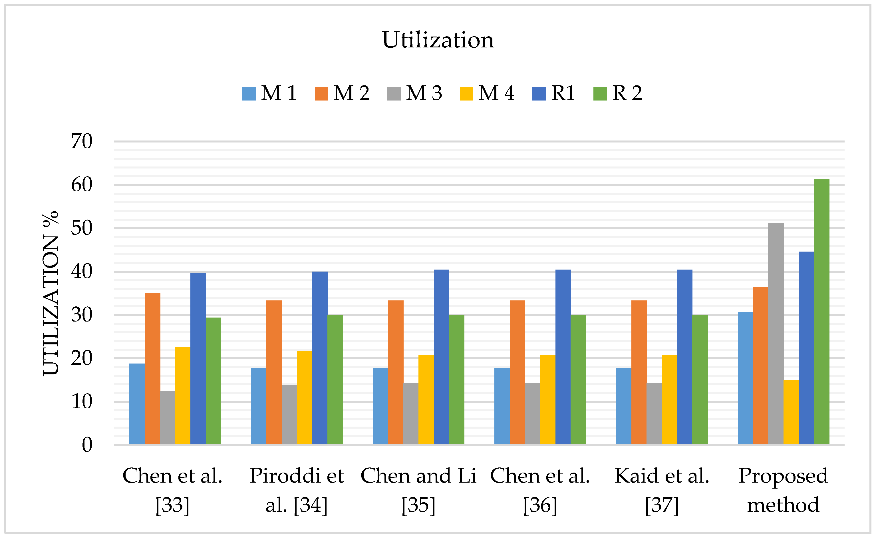
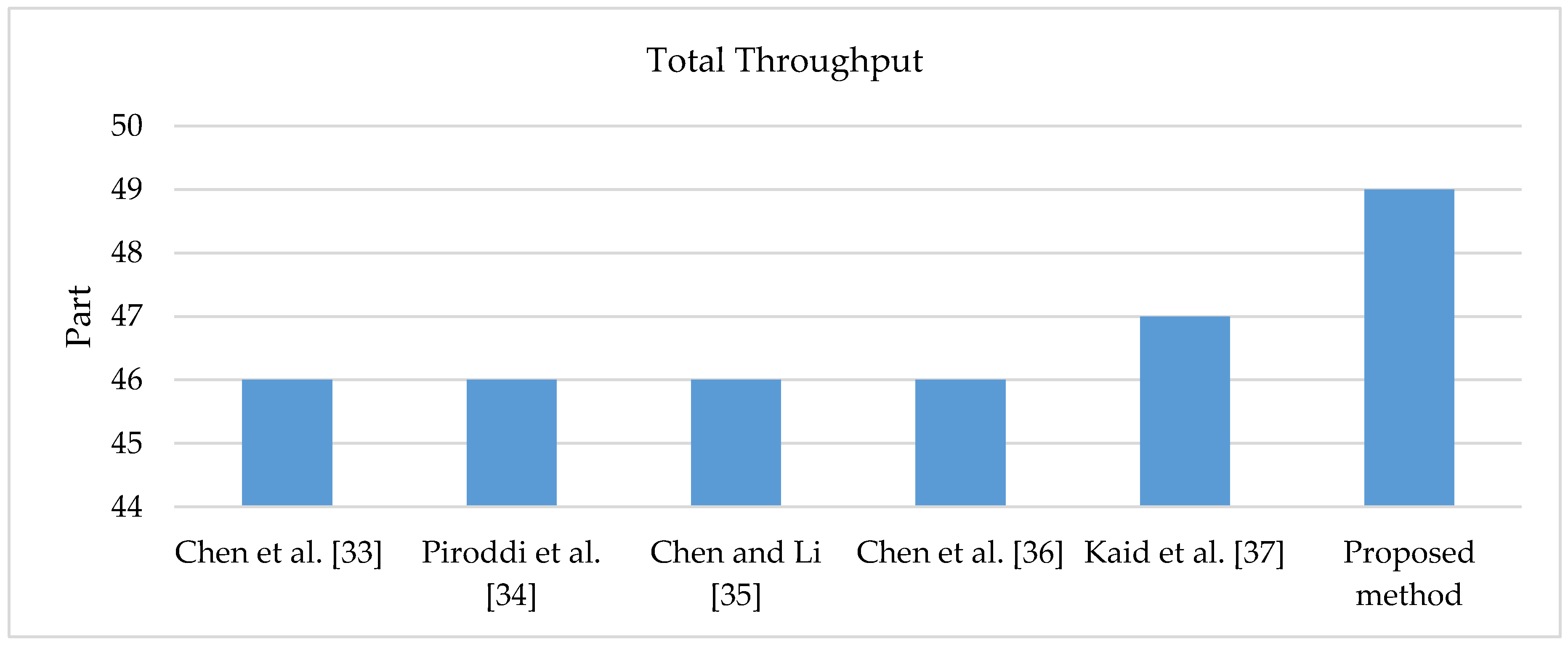
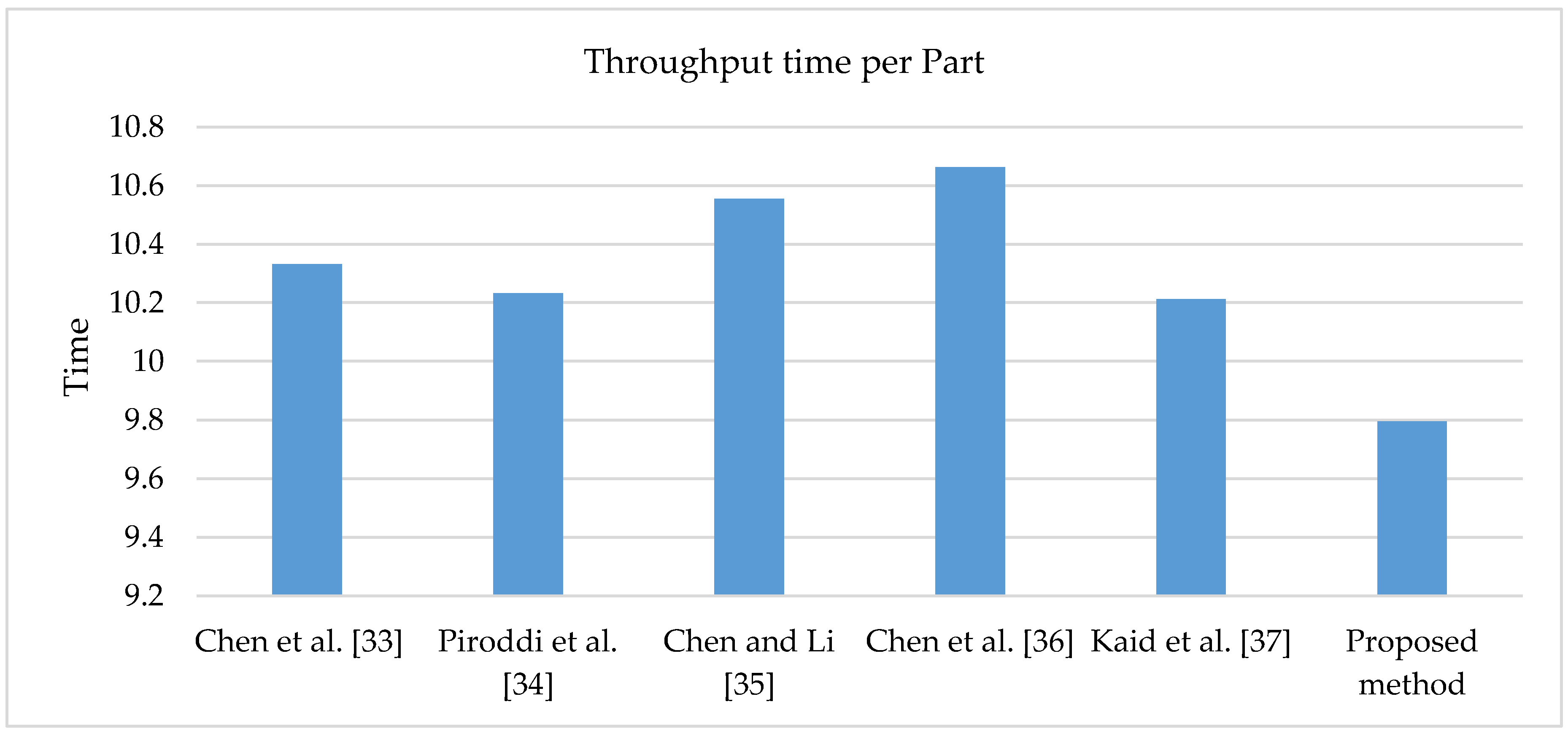
Parameter	Chen et al. [33]	Piroddi et al. [34]	Chen and Li [35]	Chen et al. [36]	Kaid et al. [37]	Proposed ICTPN Model
M 1 utilization%	18.75	17.7083	17.7083	17.7083	17.7083	30.625
M 2 utilization%	35	33.3333	33.3333	33.3333	33.9583	36.4583
M 3 utilization%	12.5	13.75	14.375	14.375	12.5	51.25
M 4 utilization%	22.5	21.6667	20.8333	20.8333	22.5	15
R 1 utilization%	39.5833	40	40.4167	40.4167	39.5833	44.583
R 2 utilization%	29.375	30	30	30	30	61.25
Total throughput of Parts	46	46	46	46	47	49
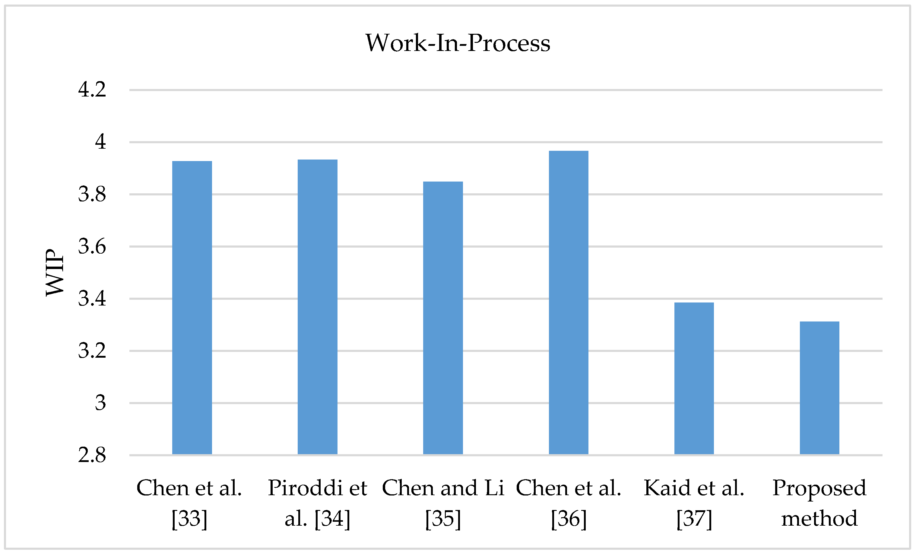
Work-In-Process	3.9271	3.93331	3.8480	3.9667	3.3854	3.31222
Throughput time per part (min)	10.3321	10.2325	10.5554	10.6635	10.2127	9.7959

. Table 2 illustrates the results in terms of the aforementioned time performance criteria. In terms of the resource utilization, overall, the proposed model can obtain better utilization than the other techniques, as illustrated in Figure 10. Moreover, from the viewpoint the throughput, the proposed model can provide greater throughput than the other techniques, as illustrated in Figure 11. With respect to the throughput time per part, the proposed model can obtain less throughput time than other techniques, as illustrated in Figure 12. Finally, in terms of WIP, the proposed model leads to better WIP than the other techniques, as illustrated in Figure 13.

4.6. Computational Complexity

Algorithm 1 models an ICTPN with N = (P_A ∪ {p_o} ∪ {p_r}, T, F, W, M_o, K, Ψ(p, c_pi, c_ti, d)). Algorithm 1 is used to model the operation and transportation resources and initial marking of the ICTPN. Obviously, all possible routes OR = {OR₁, OR₂, OR₃, …, OR_n} in a system for all types of parts are modeled. Based on the fact that each route OR in a system has R_o → R_i1 → R_i2 → ……→ R_iFi → R_o. Each sub-route R requires place p_a that corresponds to R_i(j-1), place p_a that corresponds to R_ij, and transition t, an arc from p_a to t, an arc from t to p_b, an arc from common place p_r to t, and an arc from t to common place p_r. Note that one common transportation resource p_r is added and represents all transportation resources in the system. Therefore, let x be the number of possible routes, OR, i.e., |OR| = x. The number of each sub-route F_i is expressed by y, i.e., |F_i| = y. The number of corresponding places, transitions, and arcs to each sub-route is expressed by I, i.e., |I| = z. The number of transportation resources p_r is 1, i.e., |p_r| = 1. The “FOR loop” is executed (xyz) times to model an ICTPN. Thus, the computational complexity is O(xyz). In the proposed algorithm by Wu and Zhou [6], all transportation resources are required to be added; thus, the number of transportation resources p_ri is expressed as k, i.e., |p_ri| = k. Therefore, the computational complexity of the proposed algorithm in the study of Wu and Zhou [6] is O(xyz + k). Thus, Algorithm 1 has minimal computational complexity compared with that of Wu and Zhou [6] and can be implemented in a large-scale system. In fact, Algorithm 1 has polynomial time complexity.

5. Conclusions

This paper presented a new model named an intelligent colored token Petri net for automatic reconfiguration of RMS to face the dynamical changes in the manufacturing system. The main idea is that intelligent colored tokens denote product types that represent real-time knowledge about changes and status of a system. Thus, dynamical configurations of a system can be effectively modelled. The developed ICTPN can model dynamical changes of a system in a modular manner, resulting in an easily compact model. In addition, when configurations appear, only the changed colored token from the current model has to be modified. The developed ICTPN model was tested and validated using the GPenSIM tool and compared with the existing methods from the literature.

The main advantages of the proposed method are: (1) The proposed ICTPN model is more powerful, has a simpler structure, does not need to calculate reachability graphs, and has low-overhead computation compared with Chen et al. [33], Piroddi et al. [34], Chen and Li [35], Chen et al. [36], and Kaid et al. [37]. (2) It can easily handle any dynamical changes in RMS compared with Lee and Tilbury [4], Li et al. [5], and Wu and Zhou [6]. (3) It can obtain one common transportation resource place to transport all part types compared with Wu and Zhou [6]. (4) GPenSIM code is developed for simulation, validation, and performance comparison compared with Li et al. [5], and Wu and Zhou [6]. (5) The proposed ICTPN model can dynamically change the structure of a PN without damaging its behavioral properties, i.e., liveness, conservativeness, boundedness, and reversibility. (6) We provided a representation of a RMS configuration and presented an ICTPN model for designing a modular. (7) The proposed ICTPN model can be applicable to other types of complex AMSs such as semiconductor fabrication system and liquid-crystal display factory, including automated storage and retrieval systems, automated guided vehicle, and machines. (8) The proposed ICTPN model can consider systems with sequential and complex resource requirements.

The main limitation of the proposed method is that the the ICTPN model lacks an efficient conversion method from the ICTPN model into industrial control languages for application. Therefore, our future research will investigate the proposed model to have an automatic way to test the applicability of the ICTPN model for real world systems. It is crucial to come up with a means to convert the ICTPN model into ladder diagrams (LDs) for implementation on programmable logic controllers (PLCs) [24], using adaptive control techniques [39], or using surveillance systems [40]. We will also consider to model and schedule automated manufacturing systems [41] and social networks [42] using the proposed model methodology.

References

- Mehrabi, M.G.; Ulsoy, A.G.; Koren, Y. Reconfigurable manufacturing systems: Key to future manufacturing. J. Intell. Manuf. 2000, 11, 403–419. [Google Scholar] [CrossRef]
- Katz, R. Design principles of reconfigurable machines. Int. J. Adv. Manuf. Technol. 2007, 34, 430–439. [Google Scholar] [CrossRef]
- Patel, R.; Gojiya, A.; Deb, D. Failure reconfiguration of pumps in two reservoirs connected to overhead tank. In Innovations in Infrastructure; Springer: Berlin/Heidelberg, Germany, 2019; pp. 81–92. [Google Scholar]
- Lee, S.; Tilbury, D.M. Deadlock-free resource allocation control for a reconfigurable manufacturing system with serial and parallel configuration. IEEE Trans. Syst. Man Cybern. Part C (Appl. Rev.) 2007, 37, 1373–1381. [Google Scholar] [CrossRef]
- Li, J.; Dai, X.; Meng, Z. Automatic reconfiguration of petri net controllers for reconfigurable manufacturing systems with an improved net rewriting system-based approach. IEEE Trans. Autom. Sci. Eng. 2009, 6, 156–167. [Google Scholar] [CrossRef]
- Wu, N.; Zhou, M. Intelligent token petri nets for modelling and control of reconfigurable automated manufacturing systems with dynamical changes. Trans. Inst. Meas. Control 2011, 33, 9–29. [Google Scholar]
- Târnaucă, B.; Puiu, D.; Comnac, V.; Suciu, C. Modelling a flexible manufacturing system using reconfigurable finite capacity petri nets. In Proceedings of the 2012 13th International Conference on. Optimization of Electrical and Electronic Equipment (OPTIM), Brasov, Romania, 24–26 May 2012; pp. 1079–1084. [Google Scholar]
- Kahloul, L.; Bourekkache, S.; Djouani, K.; Chaoui, A.; Kazar, O. Using high level petri nets in the modelling, simulation and verification of reconfigurable manufacturing systems. Int. J. Softw. Eng. Knowl. Eng. 2014, 24, 419–443. [Google Scholar] [CrossRef]
- Berthomieu, B.; Ribet, P.-O.; Vernadat, F. The tool tina–construction of abstract state spaces for petri nets and time petri nets. Int. J. Prod. Res. 2004, 42, 2741–2756. [Google Scholar] [CrossRef]
- Bonet, P.; Catalina, M.L.; Puigjaner, R. A petri net tool for performance modeling. In Proceedings of the 23rd Latin American Conference on Informatics, San Jose, Costa Rica, 10–11 October 2007. [Google Scholar]
- Da Silva, R.M.; Benítez-Pina, I.F.; Blos, M.F.; Santos Filho, D.J.; Miyagi, P.E. Modeling of reconfigurable distributed manufacturing control systems. IFAC Pap. 2015, 48, 1284–1289. [Google Scholar] [CrossRef]
- Yu, Z.; Guo, F.; Ouyang, J.; Zhou, L. Object-oriented petri nets and π-calculus-based modeling and analysis of reconfigurable manufacturing systems. Adv. Mech. Eng. 2016, 8, 1687814016677698. [Google Scholar] [CrossRef]
- Chao, D.Y. Fewer monitors and more efficient controllability for deadlock control in s3pgr2 (systems of simple sequential processes with general resource requirements). Comput. J. 2010, 53, 1783–1798. [Google Scholar] [CrossRef]
- Chao, D.Y. Improvement of suboptimal siphon-and fbm-based control model of a well-known s3pr. IEEE Trans. Autom. Sci. Eng. 2011, 8, 404–411. [Google Scholar] [CrossRef]
- Li, Z.; Zhou, M. Elementary siphons of petri nets and their application to deadlock prevention in flexible manufacturing systems. Syst. Man Cybern. Part A Syst. Hum. IEEE Trans. 2004, 34, 38–51. [Google Scholar] [CrossRef]
- Uzam, M. An optimal deadlock prevention policy for flexible manufacturing systems using petri net models with resources and the theory of regions. Int. J. Adv. Manuf. Technol. 2002, 19, 192–208. [Google Scholar] [CrossRef]
- Uzam, M.; Zhou, M. Iterative synthesis of petri net based deadlock prevention policy for flexible manufacturing systems. In Proceedings of the 2004 IEEE International Conference on Systems, Man and Cybernetics, The Hague, The Netherlands, 10–13 October 2004; pp. 4260–4265. [Google Scholar]
- Pan, Y.-L.; Tseng, C.-Y.; Row, T.-C. Design of improved optimal and suboptimal deadlock prevention for flexible manufacturing systems based on place invariant and reachability graph analysis methods. J. Algorithms Comput. Technol. 2017, 11, 261–270. [Google Scholar] [CrossRef]
- Zhao, M.; Uzam, M. A suboptimal deadlock control policy for designing non-blocking supervisors in flexible manufacturing systems. Inf. Sci. 2017, 388, 135–153. [Google Scholar] [CrossRef]
- Cong, X.; Gu, C.; Uzam, M.; Chen, Y.; Al-Ahmari, A.M.; Wu, N.; Zhou, M.; Li, Z. Design of optimal petri net supervisors for flexible manufacturing systems via weighted inhibitor arcs. Asian J. Control 2018, 20, 511–530. [Google Scholar] [CrossRef]
- Abdulaziz, M.; Nasr, E.A.; Al-Ahmari, A.; Kaid, H.; Li, Z. Evaluation of deadlock control designs in automated manufacturing systems. In Proceedings of the 2015 International Conference on Industrial Engineering and Operations Management, Dubai, UAE, 3–5 March 2015. [Google Scholar]
- Wang, S.; You, D.; Zhou, M. A necessary and sufficient condition for a resource subset to generate a strict minimal siphon in S 4PR. IEEE Trans. Autom. Control 2017, 62, 4173–4179. [Google Scholar] [CrossRef]
- Zhuang, Q.; Dai, W.; Wang, S.; Du, J.; Tian, Q. An mip-based deadlock prevention policy for siphon control. IEEE Access 2019, 7, 153782–153790. [Google Scholar] [CrossRef]
- Kaid, H.; Al-Ahmari, A.; El-Tamimi, A.M.; Abouel Nasr, E.; Li, Z. Design and implementation of deadlock control for automated manufacturing systems. S. Afr. J. Ind. Eng. 2019, 30, 1–23. [Google Scholar] [CrossRef]
- Nasr, E.A.; El-Tamimi, A.M.; Al-Ahmari, A.; Kaid, H. Comparison and evaluation of deadlock prevention methods for different size automated manufacturing systems. Math. Probl. Eng. 2015, 501, 1–19. [Google Scholar] [CrossRef]
- Sun, D.; Chen, Y.; El-Meligy, M.A.; Sharaf, M.A.F.; Wu, N.; Li, Z. On algebraic identification of critical states for deadlock control in automated manufacturing systems modeled with petri nets. IEEE Access 2019, 7, 121332–121349. [Google Scholar] [CrossRef]
- Al-Ahmari, A.; Kaid, H.; Li, Z.; Davidrajuh, R. Strict minimal siphon-based colored petri net supervisor synthesis for automated manufacturing systems with unreliable resources. IEEE Access 2020, 8, 22411–22424. [Google Scholar] [CrossRef]
- Li, L.; Basile, F.; Li, Z. An approach to improve permissiveness of supervisors for gmecs in time petri net systems. IEEE Trans. Autom. Control 2019, 65, 237–251. [Google Scholar] [CrossRef]
- Liu, Y.; Cai, K.; Li, Z. On scalable supervisory control of multi-agent discrete-event systems. Automatica 2019, 108, 108460. [Google Scholar] [CrossRef]
- Chen, Q.; Yin, L.; Wu, N.; El-Meligy, M.A.; Sharaf, M.A.F.; Li, Z. Diagnosability of vector discrete-event systems using predicates. IEEE Access 2019, 7, 147143–147155. [Google Scholar] [CrossRef]
- Wang, D.; Wang, X.; Li, Z. Nonblocking supervisory control of state-tree structures with conditional-preemption matrices. IEEE Trans. Ind. Inform. 2019, 16, 3744–3756. [Google Scholar] [CrossRef]
- Hu, Y.; Ma, Z.; Li, Z. Design of supervisors for active diagnosis in discrete event systems. IEEE Trans. Autom. Control 2020. [Google Scholar] [CrossRef]
- Chen, Y.; Li, Z.; Khalgui, M.; Mosbahi, O. Design of a maximally permissive liveness-enforcing petri net supervisor for flexible manufacturing systems. Autom. Sci. Eng. IEEE Trans. 2011, 8, 374–393. [Google Scholar] [CrossRef]
- Piroddi, L.; Cordone, R.; Fumagalli, I. Selective siphon control for deadlock prevention in petri nets. Syst. Man Cybern. Part A Syst. Hum. IEEE Trans. 2008, 38, 1337–1348. [Google Scholar] [CrossRef]
- Chen, Y.; Li, Z. Design of a maximally permissive liveness-enforcing supervisor with a compressed supervisory structure for flexible manufacturing systems. Automatica 2011, 47, 1028–1034. [Google Scholar] [CrossRef]
- Chen, Y.; Li, Z.; Zhou, M. Behaviorally optimal and structurally simple liveness-enforcing supervisors of flexible manufacturing systems. Syst. Man Cybern. Part A Syst. Hum. IEEE Trans. 2012, 42, 615–629. [Google Scholar] [CrossRef]
- Kaid, H.; Al-Ahmari, A.; Li, Z.; Davidrajuh, R. Single controller-based colored petri nets for deadlock control in automated manufacturing systems. Processes 2020, 8, 21. [Google Scholar] [CrossRef]
- Davidrajuh, R. Modeling Discrete-Event Systems with Gpensim: An Introduction; Springer: Berlin/Heidelberg, Germany, 2018. [Google Scholar]
- Tao, G. Adaptive Control Design and Analysis; John Wiley & Sons: Hoboken, NJ, USA, 2003; Volume 37. [Google Scholar]
- Upadhyay, J.; Deb, D.; Rawat, A. Design of smart door closer system with image classification over WLAN. Wirel. Pers. Commun. 2019, 111, 1941–1953. [Google Scholar] [CrossRef]
- Zan, X.; Wu, Z.; Guo, C.; Yu, Z. A pareto-based genetic algorithm for multi-objective scheduling of automated manufacturing systems. Adv. Mech. Eng. 2020, 12, 1–15. [Google Scholar] [CrossRef]
- Yang, L.; Li, Z.; Giua, A. Containment of rumor spread in complex social networks. Inf. Sci. 2020, 506, 113–130. [Google Scholar] [CrossRef]