Optimization Strategies for Dockless Bike Sharing Systems via two Algorithms of Closed Queuing Networks

Abstract

The dockless bike sharing system (DBSS) has been globally adopted as a sustainable transportation system. Due to the robustness and tractability of the closed queuing network (CQN), it is a well-behaved method to model DBSSs. In this paper, we view DBSSs as CQNs and use the mean value analysis (MVA) algorithm to calculate a small size DBSS and the flow equivalent server (FES) algorithm to calculate the larger size DBSS. This is the first time that the FES algorithm is used to study the DBSS, by which the CQN can be divided into different subnetworks. A parking region and its downlink roads are viewed as a subnetwork, so the computation of CQN is reduced greatly. Based on the computation results of the two algorithms, we propose two optimization functions for determining the optimal fleet size and repositioning flow, respectively. At last, we provide numerical experiments to verify the two algorithms and illustrate the optimal fleet size and repositioning flow. This computation framework can also be used to analyze other on-demand transportation networks.

1. Introduction

Bike sharing systems (BSSs) are a type of smart transportation. Nowadays, there are primarily two types of BSSs. The first one, the station-based bike sharing system (SBBSS), consists of stations distributed across the city. The capacity of a station is limited. An arriving user rents a bike from a station and returns it to a destination station if there is a vacant dock. Otherwise, the user must find another station to return the bike. SBBSSs have been carried out in over 2900 cities around the world ([1]). Another type of BSS, with no fixed stations for parking bikes, is the dockless bike sharing system (DBSS). Bikes can be parked everywhere allowable without capacity limit (refer to Shi et al. [2]). The DBSSs first arose in 2014 and now they have been deployed in over 250 cities in the world. Since the difference of capacity and parking positions, the modeling and computation of the SBBSS and DBSS are their distinguishing features. In this paper, we provide research for the DBSS.

Since the BSS is large scale and dynamic, it is vital to determine an optimal fleet size. The optimal fleet size is a tradeoff between the earnings from users and maintaining cost of the BSS. Bike availability is defined to be the probability that the parking region is not empty. It is an essential task to understand the relationship between the bike availability of each parking region and the fleet size. If the fleet is in surplus, it is a waste of resource and many bikes will pile up at the roadside and cause traffic congestion. It is a severe problem in China, notably for Mobike and ofo (two popular dockless bike sharing companies), who launched many bikes to compete for market share, which results in a tremendous waste of resources ([3]). Thus, in this paper we provide an optimization function to determine the optimal fleet size.

Bikes are scattered in the system asymmetrically, so repositioning is a necessary measure to preserve the sustainability of DBSS. There are two classes of repositioning strategies: static repositioning and dynamic repositioning. Static repositioning does not take into consideration the movements of bikes during the repositioning period, while dynamic repositioning considers the fluctuation of bikes during the repositioning process. This paper proposes a repositioning flow to rebalance the DBSS, which is a novel dynamic repositioning process.

Among the model technologies, the closed queuing network (CQN) is an appropriate method to study DBSSs, which can give sufficient consideration to the stochasticity of the system. CQN is well known as a suitable tool for studying complex systems. However there is a profound difficulty in theory to compute a large scale system because of the normalization constant. The mean value analysis (MVA) algorithm is a common algorithm to calculate the CQN without the normalization constant. Since there are plenty of road nodes, the number of nodes in the DBSS is huge. Based on the special construction of DBSS, we use the flow equivalent server (FES) algorithm to partition a parking region and its downlink road node into a subnetwork, which lessens the number of nodes significantly.

The contributions found in this paper are threefold: The first one is to use the CQN to describe a DBSS and propose an optimization function to find the optimal fleet size. The second one is to propose an optimization function to determine the repositioning flow. The third one is to use the FES algorithm to study the DBSS, which is the first time this algorithm is applied to analyze the DBSS by dividing a parking region and its downlink roads into a subnetwork to reduce the computation greatly.

The remainder of this paper is organized as follows. Section 2 provides the literature review. Section 3 sets system parameters and model description of the DBSS. Section 4 establishes a CQN to express the DBSS and gives the product form solution. Section 5 provides the MVA algorithm to solve the CQN. Section 6 proposes the FES algorithm to simplify the computation of the DBSS. Section 7 provides optimization functions for determining the optimal fleet size and repositioning flow. Section 8 gives numerical experiments. The conclusion is given in Section 9.

2. Literature Review

The research of fleet sizing is a vital topic of BSS. Some work has provided different ideas to determine the optimal fleet size. Kőchel et al. [4] provided a joint simulation optimization idea of fleet size and bike repositioning strategy and proposed an iterative means to obtain the fleet size. Fanti et al. [5] viewed an electric car sharing system as a CQN to determine the optimal fleet size and developed an optimization problem to maximize the system revenue aiming to find the optimal fleet size. Zhai et al. [6] proposed a sparse matrix construction solution method for determining the fleet size of the DBSS. Bazan et al. [7] studied mobility-on-demand networks, which are similar to BSS. They presented a simulation model combined with optimization function and queuing network and computed the optimal fleet size. These papers provide different methods to find the optimal fleet size. However, in order to consider the stochasticity fully, we choose the CQN to model the DBSS. We determine the optimal fleet size based on an optimization function, in which the parameters are obtained by computing the CQN.

Another important measure of BSS is repositioning management. For the static repositioning, Liu et al. [8] studied a DBSS with multiple heterogeneous vehicles, depots, and visits. Their conclusion was that the enhanced chemical reaction optimization (CRO) had better solutions than the preliminary CRO. Schuijbroek et al. [9] proposed a mixed-integer programming based on decomposing the multi-vehicle repositioning matters into single-vehicle problems. They also provided a heuristic of cluster-first route-second to mitigate its running time. For other static repositioning research, readers can refer to Szeto et al. [10], Bulhões et al. [11], Jia et al. [12], and Tang et al. [13]. Static repositioning typically can not adequately capture the surges in user demand. Thus dynamic repositioning needs to be studied sufficiently. For the dynamic repositioning, Shu et al. [14] found that repositioning execution can get an additional 15–20% trips. Caggiani et al. [15] carried out dynamic bike repositioning at a constant gap time. The aim is to get a high user satisfaction and a low repositioning cost. Legros et al. [16] developed an implementation decision-support tool to decide the number of bikes and which station to carry out the repositioning. They also proved that there is an optimal inventory level. Mellou and Jaillet [17] proposed a novel mixed-integer programming formulation to solve the dynamic repositioning problem and provided a linear programming model to capture the bike flows from all trips. The authors of these studies computed the repositioning flows requiring a huge number of trucks, but in this paper we relax this requirement by setting the availability of parking regions to a certain level. We also provide a probabilistic guarantee for meeting any given service level.

CQN is an appropriate method to model BSS. George et al. [18] modeled a vehicle rental system with fixed stations as a CQN. They analyzed the asymptotic behavior of vehicle availability and provided an optimization function for determining the optimal fleet size. Li et al. [19] analyzed an SBBSS as a virtual CQN, in which parking regions and roads were considered as “virtual nodes”. This was the first time that road nodes were analyzed in detail in the CQN. Li et al. [20] extended the CQN model of Li et al. [19] from three points: (i) from strong connections between stations to an irreducible graph of stations; (ii) from Poisson arrival of users to Markovian arrival processes; (iii) from exponential distributions of ridding-bike times on the roads to phase-type distributions. Furthermore, Li et al. [21] developed a fluid and diffusion approximation of a multiclass CQN to analyze the SBBSS. In this paper, we extend the computation of CQN by applying the MVA and FES algorithms. Further, some other important examples include Zhang et al. [22], Fricker et al. [23], Mizuno et al. [24], Calafiore et al. [25], Samet et al. [26], Iglesias et al. [27], and Vishkaei et al. [28].

3. Model Description

In this section, we give a detailed model description for the DBSS.

(1) Parking regions: In the DBSS, parking regions are viewed as nodes. Since the geographical locations and surrounding traffic environment may be different, we determine that the parking regions are different. We assume that the parking space of each parking region is sufficient so that bikes can always be parked upon arrival at a parking region immediately, that is, having no blocking effects. We assume that there are N parking regions distributed in the DBSS and denote the set of parking region nodes by $S=\left\{1,2,\dots ,N\right\}$.

(2) Roads: Parking regions are connected by roads. We express the set of roads as I. Since there are origin-direction links of parking regions, we view the roads between parking regions are directed. Road $i\to j$ and Road $j\to i$ are different roads for $1\le i,j\le N$. We view Road $i\to j$ as a node with finite servers and assume that the travel time from Parking region i to Parking region j is exponential with mean random variable $1/{\mu }_{ij}$.

We denote the set of downlink parking regions of Parking region i by ${\mathsf{\Theta }}_i$. Similarly, we denote the set of uplink parking regions of Parking region i by ${\mathsf{\Delta }}_i$.

To express the set of parking regions starting from Parking region i for $1\le i\le N$, we write

$$R\left(i\right)=\left\{\mathrm{Road}i\to j:j\in {\mathsf{\Theta }}_i\right\}.$$

The number of directed roads in the set $R\left(i\right)$ at most is $N-1$. The number of elements in the set $R\left(i\right)$ is $\left|R\left(i\right)\right|$. We let $M={\sum }_{i=1}^N\left|R\left(i\right)\right|$, thus $M\le N\left(N-1\right)$.

We assume that there is an irreducible path in the DBSS. The irreducibility is guaranteed by a suitable road construction with $R\left(i\right)$ for $1\le i\le N$. The set of road nodes is denoted by $I=\left\{N+1,N+2,\dots ,M\right\}$. For the detailed expression of irreducible path, readers can refer to Li et al. [20].

(3) User arrival processes: We assume that the arrivals of users at Parking region i is a Poisson process and set the mean arrival rate as ${\lambda }_i>0$ for $1\le i\le N$.

(4) Bike using processes: When a user arrives at Parking region i with at least one bike, he rents a bike and rides it on the Road $i\to j$ with probability $p_{ij}$ for $j\in {\mathsf{\Theta }}_i$ and ${\sum }_{j\in {\mathsf{\Theta }}_i}{p}_{ij}=1$ for each $i=1,2,\dots ,N$. The service times on the Road $i\to j$ are i.i.d. and exponential with mean rate ${\mu }_{ij}>0$.

(5) The departure discipline: The users will leave the system with two cases: (i) when a user arrives at a parking region that has no bikes, he will leave the system directly. (b) When a user finishes his trip and returns the bike to a parking region successfully, he leaves the system immediately.

All the random variables above are independent of each other.

At each parking region, bikes form a queue while waiting for users to rent. Thus, from the perspective of bikes, we consider the parking regions as single-server (SS) nodes and the roads as finite-server (FS) nodes (the number of the servers on the road is less than or equal to the total number of bikes in the DBSS). Parking region i can be viewed as a server with service rate ${\lambda }_i$ and follows First Come First Served (FCFS) scheduling for $1\le i\le N$. The service time of a parking region is the interval time of customer arrival. A bike leaves an SS node and moves to an FS node. Parking region nodes are viewed as M/M/1 queuing systems, while road nodes are modeled as M/M/n queuing systems. Figure 1 illustrates a DBSS with three parking regions.

4. Closed Queuing Network

All the bikes are just circulating among parking regions and roads in the DBSS, and the number of bikes in a DBSS is fixed. From bikes’ perspective, we model the DBSS as a closed queuing network.

First, we let $n_i\left(t\right)$ denote the number of bikes in Node i at time t and $\mathbf{Q}\left(t\right)=\left(n_1\left(t\right),n_2\left(t\right),\cdots ,n_{N+M}\left(t\right)\right)$. Thus $\left\{\mathbf{Q}\left(t\right):t\ge 0\right\}$ is a Markov process. When a user rents a bike at Parking region i, he selects a destination of Parking region j with probability $p_{ij}$, where $p_{ij}>0$, $p_{ii}=0$, and ${\sum }_{j\in {\mathsf{\Theta }}_i}{p}_{ij}=1$. For each $i\in I$, we define $u\left(i\right)$ and $d\left(i\right)$ to be the uplink and downlink nodes of i, which denote the origin and destination nodes of i, respectively. The elements of routing matrix P are written as

$$f_{ij}=\left\{\begin{array}{cc}{p}_{ij},\hfill & i\in S,j\in I,i=u\left(j\right),\hfill \\ 1,\hfill & i\in I,j\in S,i=d\left(j\right),\hfill \\ 0,\hfill & \mathrm{otherwise}.\hfill \end{array}\right.$$

The service time of each node is exponential. For $i\in S$, ${\mu }_i={\lambda }_i$. For Node $i\to j$, ${\mu }_{ij}=n_{ij}{\mu }_{ij}$ where $n_{ij}$ is the number of bikes on Node $i\to j$.

We set $n_i$ as the number of bikes in Node i. To study the CQN, the service rates, the routing matrix and relative arrival rates are needed to be determined first. For a given fleet size K, the state space of the CQN is $\mathsf{\Omega }=\left\{\mathbf{n}:{\sum }_{i=1}^{N+M}{n}_i\left(t\right)=K,0\le n_i\le K\right\}$, where $\mathbf{n}=\left(n_1,n_2,\dots n_N,n_{N+1},n_{N+2},\dots ,n_{N+M}\right)$. The relative arrival rate $e_i$ is written as

$$e_j=\sum _{i=1}^{N+M}{e}_i{f}_{ij}.$$

(1)

Our network consists of finite-server nodes and single-server nodes with exponential service time, so this model is a BCMP network, which has a product form solution (See Baskett et al. [29]). The product form solution is given by

$$\mathsf{\beta }\left(\mathbf{n}\right)=\frac{1}{G}\prod _{i=1}^{N+M}{\mathsf{\beta }}_i\left(n_i\right),$$

(2)

in which

$${\mathsf{\beta }}_i\left(n_i\right)=\left\{\begin{array}{cc}{\left(\frac{e_i}{{\lambda }_i}\right)}^{n_i},& i\in S,\\ {\left(\frac{e_i}{{\mu }_i}\right)}^{n_i}\frac{1}{n_i!},& i\in I.\end{array}\right.$$

Note that $\mathbf{n}\in \mathsf{\Omega }$ and

$$G=\sum _{\mathbf{n}\in \mathsf{\Omega }}\prod _{i=1}^{N+M}{\mathsf{\beta }}_i\left(n_i\right).$$

For the detailed proof of the product form solution, readers can refer to Baskett et al. [29]. For the DBSS, there are two vital performance measures:

(1) Expected revenue E charged by the bikes on roads

$$E=K-\sum _{i\in S}{n}_i.$$

(2) Service level $A_i$ measured by the mean bike availability

$$A_i=1-p\left(n_i=0\right),i\in S.$$

Expected revenue E is the utmost concern of operators. The value $A_i$ is an acknowledged measure of the quality of service. Incentive measures can be implemented based the results of $A_i$. For example, measures include guiding customers to rent bikes at parking regions with high relative utilization and return bikes to parking regions with lower utilization.

5. MVA Algorithm of the Closed Queuing Network

Since the computation of normalization constant G is expensive, we apply the MVA algorithm (see Reiser and Lavenberg [30]) to compute the CQN by avoiding the calculating of the normalization constant. Through the MVA algorithm, we can calculate the mean waiting times ${\overline{T}}_i\left(k\right)$ and the mean queue lengths ${\overline{K}}_i\left(k\right)$ at each Node i of a CQN, where $k=1,\dots ,K$.

Based on the the MVA algorithm, we can get the mean response time at the ith node

$${\overline{T}}_i\left(k\right)=\left\{\begin{array}{cc}\frac{1}{{\mu }_i}\left[1+{\overline{K}}_i\left(k-1\right)\right],\hfill & i\in S,\hfill \\ \frac{1}{{\mu }_i},\hfill & i\in I.\hfill \end{array}\right.$$

(3)

Based on ${\overline{T}}_i\left(k\right)$, the overall throughput is given by

$$\lambda \left(k\right)=\frac{k}{{\displaystyle \sum _{i=1}^{N+M}}{e}_i{\overline{T}}_i\left(k\right)},$$

(4)

and the throughput of each node can be written as

$${\lambda }_i\left(k\right)=\lambda \left(k\right)e_i,\mathrm{for}i=1,2,\dots ,N+M,$$

(5)

in which $e_i$ is determined by Equation (1).

Based on ${\overline{T}}_i\left(k\right)$ and ${\lambda }_i\left(k\right)$, the mean number of bikes at the ith node is written as

$${\overline{K}}_i\left(k\right)={\lambda }_i\left(k\right){\overline{T}}_i\left(k\right).$$

(6)

We provide the detailed computation by MVA in Algorithm 1.

Algorithm 1 Mean value analysis (MVA) algorithm for closed queuing network.

Step 1. Initialization    ${\overline{K}}_i\left(k\right)=0,$ for $i=1,2,\dots ,N+M$. $G\left(0\right)=1.$

Step 2. Computation for the relative arrival rates    Let $e_1=1$. Compute relative arrival rates $e_j$ for $j=2,3,\dots ,N+M$, based on equation $e_j={\sum }_{i=1}^{N+M}{e}_i{p}_{ij}$ for $i=1,2,\dots ,N+M$.

Step 3. Iteration over the number of bikes in the network starting with$k=1$:

Step 3.1 Compute mean response time based on equation $\overline{T_i}\left(1\right)=\frac{1}{{\mu }_i}\left[1+\overline{K_i}\left(0\right)\right]$ for $i=1,2,\dots ,N$, and $\overline{T_i}\left(1\right)=\frac{1}{{\mu }_i}$ for $i=N+1,\dots ,N+M$.

Step 3.2 Compute the throughput based on equation $\lambda \left(1\right)=\frac{1}{{\sum }_{i=1}^{N+M}{e}_i\overline{T_i}\left(1\right)}$.    Get the normalization constant based on equation $G\left(1\right)=\frac{G\left(0\right)}{\lambda \left(1\right)}$.

Step 3.3 Compute the mean number of bikes at each node based on equation $\overline{K_i}\left(1\right)=e_i\lambda \left(1\right)\overline{T_i}\left(1\right)$.

Step 4. Iteration over the number of bikes in the network for$k=2,\dots ,K$.

Step 4.1 Compute mean response time based on equation $\overline{T_i}\left(k\right)=\frac{1}{{\mu }_i}\left[1+\overline{K_i}\left(k-1\right)\right]$ for $i=1,2,\dots ,N+M$, and $\overline{T_i}\left(k\right)=\frac{1}{{\mu }_i}$ for $i=N+1,\dots ,N+M$.

Step 4.2 Compute the throughput based on equation $\lambda \left(k\right)=\frac{k}{{\sum }_{i=1}^N{e}_i\overline{T_i}\left(k\right)}$.    Get the normalization constant based on equation $G\left(k\right)=\frac{G\left(k-1\right)}{\lambda \left(k\right)}$.

Step 4.3 Compute the mean number of bikes at each node based on equation $\overline{K_i}\left(k\right)=e_i\lambda \left(k\right)\overline{T_i}\left(k\right)$.

Step 4.4 Get $\overline{T_i}\left(K\right)$ and $\overline{K_i}\left(K\right)$ for $i=1,2,\dots ,N+M$.

Step 5. Computation for performance measures $E_i$ and $A_i$ in the closed queuing network.

We are interested in the availability of bikes at each parking region (i.e., the probability that there is at least one bike at the parking region). Set ${\overline{T}}_i\left(0\right)={\overline{K}}_i\left(0\right)=0$. By iteration, we can get

$$E_i={\overline{K}}_i\left(K\right),i=1,2,\dots ,N,$$

and

$$A_i=\frac{E_i}{1+E_i},i=1,2,\dots ,N.$$

For small networks, this algorithm provides a method to obtain the optimal fleet size straightly. However, for a larger network, the computation is too expensive. Thus, we need to find another approach to reduce the computation.

6. FES Algorithm of the Closed Queuing Network

MVA algorithm can be computed directly without calculating the normalizing constant, but it needs high storage requirement and expensive computation. So we try to find another approach to reduce the computation. We use the FES algorithm to compute the DBSS.

In the closed queuing network of DBSS, since bikes are served in parking regions as well as on roads, we divide the nodes into SS nodes and FS nodes. However, when we consider the two performance measures: expected revenue $E_i$ and available rate $A_i$, we only consider the results of SS nodes. Since the difference between parking region nodes and road nodes, we try to simplify the computation by partitioning them.

FES method is based on Norton’s theorem, refer to Chandy et al. [31] and Akyildiz et al. [32]. Based on the FES method, we partition the closed queuing network into N disjoint subnetworks, in which Node i and node $i\to j$ are a subnetwork for $i=1,\dots ,N,j\in {\mathsf{\Theta }}_i$. We write the subnetwork as $S{N}_1,S{N}_2,\dots ,S{N}_N$. Analyzing one of the subnetworks, we need to short-circuit all the other nodes that do not belong to the subnetwork.

First, we need to determine the throughput ${\lambda }_{S{N}_j}\left(k\right)$ and the normalization constant $G_j\left(k\right)$ for $1\le j\le N$ and $1\le k\le K$. The arrival rates of nodes in the subnetwork are the same as the original network. Consider each subnetwork as an FES node and construct an equivalent reduced network. The dependent service rates ${\mu }_{ej}$ of the FES Node j are identical with the throughputs in the corresponding jth subnetwork, which is written as

$${\mu }_{ej}\left(k\right)={\lambda }_{S{N}_j}\left(k\right),\mathrm{for}j=1,\dots ,N\mathrm{and}k=1,\dots ,K.$$

We provide the detailed FES in Algorithm 2. In Algorithm 2, the time and storage requirement are reduced considerably.

Algorithm 2 Flow equivalent server (FES) algorithm for closed queuing network.

Step 1. Partition the network into$\mathbf{N}$subnetworks.    Partition the network into subnetworks $S{N}_1,S{N}_2,\dots ,S{N}_N$, in which Node i and Node $i\to j$ constitute $S{N}_i$ subnetwork for $i=1,\dots ,N,j\in {\mathsf{\Theta }}_i$.

Step 2. Analyze each subnetwork and construct the reduced network    For subnetwork 1. Shot-circuit all the other subnetworks. Use the MVA algorithm to compute throughputs and the normalization constants of the subnetwork. Then we get ${\lambda }_{S{N}_1}\left(1\right),{\lambda }_{S{N}_1}\left(2\right),\dots ,{\lambda }_{S{N}_1}\left(K\right)$ and $G_1\left(1\right),G_1\left(2\right),\dots ,G_1\left(K\right)$.    Analogously, analyze subnetworks 2 to N, and obtain ${\lambda }_{S{N}_j}\left(1\right),{\lambda }_{S{N}_j}\left(2\right),\dots ,{\lambda }_{S{N}_j}\left(K\right)$ and $G_j\left(1\right),G_j\left(2\right),\dots ,G_j\left(K\right)$, for $j=2,3,\dots ,N$. We get ${\mu }_{ei}\left(k\right)={\lambda }_{S{N}_i}\left(k\right)$ for $k=1,2,\dots ,K$, and $i=2,3,\cdots ,M$.

Step 3. Compute the normalization constants.    Compute the normalization constant of the reduced network by convoluting the N normalizing vectors, based on the equation $G=G_1\otimes G_2\otimes \dots \otimes G_M$.

Step 4. Computation for performance measures in the CQN.    Compute the mean number of bikes in Node i by $\overline{K_i}\left(K\right)={\displaystyle \sum _{k=1}^K}{\left(\frac{e_i}{{\mu }_i}\right)}^k\frac{G\left(K-k\right)}{G\left(K\right)}\mathrm{for}i=1,2,\dots N$.    The utilization of Node i by ${\rho }_i\left(K\right)=\frac{e_i}{{\mu }_i}\frac{G\left(K-1\right)}{G\left(K\right)}\mathrm{for}i=1,2,\dots N$.    The mean response time of Node i by $\overline{T_i}\left(K\right)={\displaystyle \sum _{k=1}^K}{\left(\frac{e_i}{{\mu }_i}\right)}^k\frac{G\left(K-k\right)}{e_{i}G\left(K-1\right)}\mathrm{for}i=1,2,\dots N$.

7. Performance Analysis

In this section, we provide the results of a performance analysis of DBSSs. Based on the MVA and FES algorithms, we get the results of the expected number of bikes and the availability for each parking region. Then, we propose two optimization functions to determine the optimal fleet size and the repositioning flow based on the results.

7.1. Optimal Fleet Size

Since the optimal fleet size is a tradeoff between the earnings got from users and maintaining cost of the fleet, we present an optimization function to determine the optimal fleet size. Let $r_i$ be the revenue obtained from a bike being in use at road nodes per-unit-time. The BSS will cause an unavailability cost $c_j$ whenever bikes park at parking regions idly. Then the objective is to maximize the profit

$$F\left(K\right)=\underset{\left\{X_i\right\}}{max}\sum _{i\in I}{E}_i\left(K\right)r_i-\sum _{j\in S}{c}_j{\lambda }_j\left(1-A_j\left(K\right)\right),$$

(7)

in which $E_i$ is the expected queue length at Node i for $i\in I$ and $A_j$ is bike availability at Node j for $j\in S$ in steady state.

Based on Shanthikumar and Yao [33] and George et al. [18], we get that for a single-class CQN with FCFS exponential servers, both the throughput at each parking region and the system throughput are non-decreasing concave functions of fleet size. The values $\{A_j\left(K\right),j\in S\}$ and $\{E_i\left(K\right),i\in I\}$ are all non-decreasing concave functions, therefore $F\left(K\right)$ is concave.

To solve Equation (7), we can calculate the MVA algorithm iteratively for each $K\in \{1,2,\dots \}$ and compute the associated profit. Since the concavity of $F\left(K\right)$, the method will terminate once profit decreases from K to $K+1$.

7.2. Repositioning Flow

Since bikes will inevitably accumulate at one or more parking regions in the DBSS. To ease this problem, we introduce a set of repositioning flow to rebalance the system, i.e., moving bikes to parking regions that lack bikes. We use $y_{ij}$ to denote the rate of bikes repositioning flow from Parking region i to Parking region j. We discuss how to achieve a target service level with different bike resources.

We assume that $Y_i={\sum }_{j\in {\mathsf{\Theta }}_i}{y}_{ij}$. The availability of Parking region i is given by

$$A_i=\frac{e_i}{{\lambda }_i+Y_i}.$$

If we set the availability $A_i$ of Parking region i equal to 1, it needs a huge number of bikes idly waiting at each parking region to meet the availability (refer to Li et al. [34]). Thus, we set the objective as a service level min $\left\{A_i\right\}\ge \sigma \in \left(0,1\right)$. Therefore, we can realize the certain level of availability and release stressful demand of the fleet size. Then the repositioning cost minimization problem can be written by

$$\underset{\left\{X_i\right\}}{min}\sum _{i\in S}{b}_i{Y}_i{A}_i$$

$$s.t.A_i\ge \sigma ,i\in S,$$

where $b_j$ is the cost of maintaining bikes and $b_j=\sum _{j\in {\mathsf{\Theta }}_i}{b}_{ij}{p}_{ij}$.

We set ${\xi }_i=e_i/{\lambda }_i$, ${\overline{\xi }}_i=max\left\{e_i/{\lambda }_i\right\}$, ${\gamma }_i=e_i/\left({\lambda }_i+X_i\right)$, and ${\overline{\gamma }}_i=max\left\{e_i/\left({\lambda }_i+X_i\right)\right\}$ for $i\in S$. Since $A_i={\gamma }_i/{\overline{\gamma }}_i$, the optimal equation can be rewritten as

$$\underset{\left\{X_i\right\}}{min}\sum _{i\in S}{b}_i{Y}_i\frac{e_i}{{\overline{\gamma }}_i\left({\lambda }_i+Y_i\right)}$$

$$s.t.\frac{e_i}{{\overline{\gamma }}_i\left({\lambda }_i+Y_i\right)}\ge \sigma ,i\in S.$$

The optimal solution is

$$Y_i=max\left\{0,\frac{\sigma e_i}{{\overline{\xi }}_i}-{\lambda }_i\right\},i\in S.$$

8. Numerical Experiments

For the closed queuing network, the MVA algorithm can be used to compute a small size DBSS and the FES algorithm can be used to calculate larger size DBSS. We used a small size system to verify the computational accuracy of the MVA and FES algorithms. Then we provide the results of the computation of optimal fleet size and repositioning flow. For all the numerical experiments, we implemented the computation in Matlab on a laptop.

8.1. Comparison of Algorithm 1 and Algorithm 2

We studied a small size DBSS with three parking regions and the three parking regions are connected to each other and so there are six road nodes. We describe the DBSS as a CQN and set the fleet size as 45. The physical structure of the DBSS is depicted in Figure 2.

The routing matrix P is given by

$$P=\left(\begin{array}{ccccccc}& & & 0.4& & 0.6& \\ & & & & 0.3& & & 0.7\\ & & & & & & 0.6& & 0.4\\ & 1& & & \\ 1& & & & \\ & & 1& & & \\ 1& & & & \\ & & 1& & & \\ & 1& & & \end{array}\right).$$

Based on the routing matrix P and Equation (1), we can obtain relative arrival rates. We list the service rates and the relative arrival rates in

Table 1. The service rates and the relative arrival rates.

${\mathit{\mu }}_1$	${\mathit{\mu }}_2$	${\mathit{\mu }}_3$	${\mathit{\mu }}_4$	${\mathit{\mu }}_5$	${\mathit{\mu }}_6$	${\mathit{\mu }}_7$	${\mathit{\mu }}_8$	${\mathit{\mu }}_9$
10	8	6	1	3	2	4	2	6
$e_1$	$e_2$	$e_3$	$e_4$	$e_5$	$e_5$	$e_7$	$e_8$	$e_9$
1	0.8889	1.2222	0.4000	0.2667	0.6000	0.7333	0.6222	0.4889

.

Using the FES algorithm, we divided the nine nodes into three subnetworks. i.e., Node 1, Node 4 and Node 6 are subnetwork 1; Node 2, Node 5, and Node 8 are subnetwork 2; Node 3, Node 7, and Node 9 are subnetwork 3. We computed the DBSS by Algorithm 1 and 2 respectively and verified that the results are consistent. We provide the results in

Table 2. The expected number obtained by MVA and FES algorithms.

${\overline{\mathit{K}}}_1$	${\overline{\mathit{K}}}_2$	${\overline{\mathit{K}}}_3$	${\overline{\mathit{K}}}_4$	${\overline{\mathit{K}}}_5$	${\overline{\mathit{K}}}_6$	${\overline{\mathit{K}}}_7$	${\overline{\mathit{K}}}_8$	${\overline{\mathit{K}}}_9$
8.3333	15.3846	12.0376	1.3625	0.2857	2.9981	0.8461	3.4963	0.2558

.

8.2. Optimal Fleet Size and Repositioning Flow

(1) The three parking region DBSS

Let the hourly rental fee $r_i$ for $i\in I$ be $2 and the maintenance cost $c_i$ per-bike per-hour for $i\in S$ be $0.20. By Algorithm 2 and Equation (7), we compute the three parking region DBSS depicted in Figure 2. The variation of profits corresponding to fleet size is shown in Figure 3. We can find that the optimal fleet size is 60. This method considers the differences between parking regions and loose structures of the routing matrix. We can find that the profit first increases and then decreases as the fleet size K increases. This result offers operators quantitative basis of the fleet size design.

When setting ${\min }_{i\in S}\left\{A_i\right\}\ge 0.9$, we get the optimal repositioning strategy to add rebalancing flows $1\to 4$ with a rate of 0.0641, $1\to 6$ with a rate of 0.0547, and $3\to 8$ with a rate of 0.1431. The ${\min }_{i\in S}\left\{A_i\right\}\ge 0.9$. The computation of repositioning flow considers the dynamics of DBSS, which is close to the actual operation.

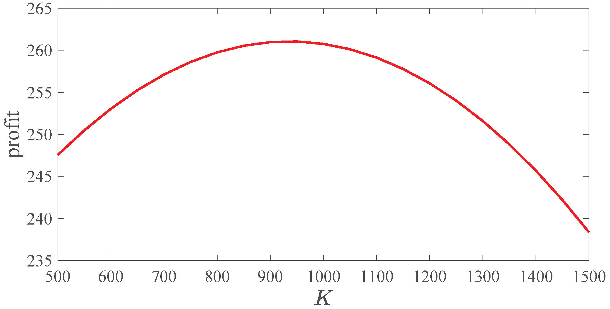
(2) A 50 parking region DBSS

By Algorithm 2, we computed a DBSS with 50 parking regions. We partitioned the DBSS into 50 subnetworks and depict the optimal fleet size in Figure 4. The optimal repositioning flows are listed in

Table 3. The expected number obtained by MVA and FES algorithms.

$y_{1,2}$	$y_{4,5}$	$y_{8,7}$	$y_{10,9}$	$y_{11,10}$	$y_{13,14}$	$y_{17,18}$	$y_{24,23}$	$y_{25,26}$	$y_{28,27}$
1.3513	2.3468	2.0276	0.3215	1.8527	1.9812	0.4621	2.9613	0.0358	1.7852
$y_{29,30}$	$y_{31,32}$	$y_{35,36}$	$y_{37,36}$	$y_{39,40}$	$y_{41,40}$	$y_{43,42}$	$y_{44,45}$	$y_{47,48}$	$y_{50,1}$
1.4562	0.1383	1.8246	1.0037	1.6125	0.2471	2.8132	0.8160	3.2613	1.8421

, in which $y_{i,j}$ is the flow from Parking region i to Road $i\to j$. Algorithm 2 extends the computation of CQN of DBSS greatly. Since there are actual service processes on the road in the DBSS, when we analyze the system we must study the service rates on the road nodes. It is well known that the number of road nodes is enormous in a DBSS, which will cause the state space explosion and lead to the computation of normalization constant too expensive. By partitioning the system into subnetworks, the number of nodes is reduced significantly, which realizes the performance computation of larger size DBSS. Thus the result provides operators with valuable quantitative reference.

9. Conclusions

In this paper, we provide a closed queuing network of dockless bike sharing systems. To avoid the expensive computation of the normalization constant, we use the MVA algorithm and the FES algorithm to analyze the small size and larger size DBSS, respectively. The FES algorithm is proposed to compute the DBSS for the first time. We let a parking region and its downlink roads as a subnetwork and partition the DBSS into different subnetworks. The FES algorithm reduces the number of nodes greatly, and thus the computation of the CQN is lessened significantly. This paper opens a new avenue to study the CQN of DBSS. Based on the computation results of the CQN, we determine the optimal fleet size and repositioning flow by two optimization functions. The computation of repositioning flow adequately considers the dynamics of bikes during the repositioning process, which is close to the actual DBSS. According to our analysis, the method can be used as guidelines for designing and controlling the fleet and arrange the repositioning flow to achieve a high level of service.

For future work, the CQN model presented in this paper can be used to analyze other on-demand transportation networks. Another upcoming issue is that we can consider the unusable bikes in the DBSS. Since the failure rates of bikes are high, unusable bikes account for a large proportion in the DBSS. Therefore when determining the optimal fleet and the repositioning flow, the failure rate of bikes can be introduced in.