A New Improved Learning Algorithm for Convolutional Neural Networks

Abstract

The back-propagation (BP) algorithm is usually used to train convolutional neural networks (CNNs) and has made greater progress in image classification. It updates weights with the gradient descent, and the farther the sample is from the target, the greater the contribution of it to the weight change. However, the influence of samples classified correctly but that are close to the classification boundary is diminished. This paper defines the classification confidence as the degree to which a sample belongs to its correct category, and divides samples of each category into dangerous and safe according to a dynamic classification confidence threshold. Then a new learning algorithm is presented to penalize the loss function with danger samples but not all samples to enable CNN to pay more attention to danger samples and to learn effective information more accurately. The experiment results, carried out on the MNIST dataset and three sub-datasets of CIFAR-10, showed that for the MNIST dataset, the accuracy of Non-improve CNN reached 99.246%, while that of PCNN reached 99.3%; for three sub-datasets of CIFAR-10, the accuracies of Non-improve CNN are 96.15%, 88.93%, and 94.92%, respectively, while those of PCNN are 96.44%, 89.37%, and 95.22%, respectively.

1. Introduction

With the improvement of the computational processing capabilities and the growth of data, deep learning approaches [1] have attracted extensive attention. In particular, CNN [2] makes a huge contribution in object detection [3], image classification [4], semantic segmentation [5], and so on. All this is attributed to its ability of constructing high-level features from low-level ones, so as to learn the feature hierarchy of images.

To boost the performance of CNN, the existing strategies usually attempt from two aspects. One is finding substitutes of some blocks or functions to optimize the network structure. Sun et al. [6] introduced a new companion objective function as a regularization strategy, mainly supervising convolution filters and nonlinear activation functions. Srivastava et al. proposed the Dropout method [7], which randomly discarded neurons from the neural network with a certain probability during training, effectively alleviating the over-fitting. Simonyan and Zisserman [8] showed that it was feasible to improve classification results by increasing the depth and width of the network. Szegedy et al. [9] introduced the inception model, which mainly generated diverse visual features by combining various sizes of convolution kernels. Kechagias-Stamatis et al. [10] proposed a new structure combining convolutional neural network with sparse coding to achieve the highest performance in the field of automatic target recognition.

The other research aspect is to optimize learning algorithms for CNN. The BP algorithm [11] is often used to train CNN, which updates parameters by calculating the gradient of the loss function. The derivation details can be found in [12]. The parameter updating equations in CNN are different than the traditional ones in that the partial derivative of the ReLU activation function [13] of the convolutional layer is 1 if the feature map produced by the convolution is greater than 0; otherwise, it is 0. If the convolution filter element is not activated initially, then they are always in the off-state as zero gradients flow through them. So the introduction of the ReLU alleviates the disappearance of gradients, but also makes the network sparse and results in many convolution filter elements lost the updating chances in the back propagation.

There are some existing literatures trying to overcome this disadvantage. Maas et al. [14] proposed Leaky ReLU activation function whose gradient was a constant instead of 0 if the input of ReLU was negative. Xu et al. [15] introduced Randomized Leaky ReLU (RReLU), a variant of Leaky ReLU, in which the slope of the negative neuron is randomly selected from a uniform distribution in training but is fixed in test. He et al. [16] replaced the ReLU with Parametric Rectified Linear Unit (PReLU), in which the gradient of the negative neuron is a parameter that can be learned, to provide effective information for negative neurons as well as to solve the gradient vanishing problem in deep networks. Goodfellow et al. [17] proposed Maxout activation function which does not suffer from the dying convolution filter element because gradient always flows through every maxout neuron even when a maxout neuron is 0, this 0 is a function of the parameters and may be adjusted. Neurons that take on negative activation may be steered to become positive again later.

All above researches focus on improving or replacing the ReLU to boost the BP for CNN. But they also have some problems, such as unstable performance, less versatile, high computing expense, and so on. So some researchers have paid attention to improving information extraction on training samples. In [18], the learning coefficients of correctly classified and misclassified samples were reduced and enhanced, respectively. With this trick, samples, around the classification boundary but correctly classified, contribute less to training than before but in fact they have a lot of information to be learned. Lin et al. [19] proposed a new loss function, Focal loss, which is a modification of the standard cross-entropy loss function. The Focal loss function can not only solve the problem of class imbalance, but also make the model focus more on misclassified samples during the training by reducing the weight of samples that are easy to classify. Moghimi et al. [20] used CNN as the basic classifier in boosting, and adjusted the weight of all samples after each iteration, so as to pay more attention to the misclassified samples in the next training. Guo et al. [21] designed a random drop loss function, which randomly abandoned negative samples according to their classification difficulty, that is, easy samples were discarded, while samples that are difficult to be classified were trained again, so that the updating of weights are more affected by the difficult samples. However, there are always some samples classified correctly but around at the classification boundary during the training process. They are deprived of or lowered the chance that they will be learned. It seems arbitrary to use the classification boundary to determine whether a sample should be studied intensively. In addition, misclassified boundary samples should also be learned more. In general, to compensate for the sparsity caused by the ReLU, the importance of difficult to classify samples and other misclassified samples should be strengthened during the training of CNN.

Motivated by the above, this paper improves the BP algorithm of CNN by involving a penalty term with a new concept, the classification confidence, which describes the degree of one sample belonging to its target category. The lower the classification confidence of the sample, the more likely the sample is to fall near the classification boundary and even be misclassified. Considering that each sample of a category has different classification confidence during the training process, the network should learn more from the sample with low classification confidence.

The rest of this paper is organized as follows. Section 2 briefly introduces the structure of CNN. Then, the new learning method is presented in Section 3. The relevant experimental results are reported and discussed in Section 4. Finally, the conclusions and ideas of future research are introduced.

2. Convolutional Neural Network

CNN is a special multilayer feedforward neural network designed to deal with image data. It has the characteristics of sparse interaction and parameter sharing [22]. Inspired by biological visual neural networks, the sparse interaction means that each hidden neuron only connects a small piece of adjacent area of the input image; the parameter sharing allows the convolution filter to share the same weight matrix and bias in the process of convolving the input image, ensuring the translation invariance of the image and reducing the number of weight parameters. The CNN is mainly composed of convolutional layers, pooling layers and fully connected layers. The structure of a typical CNN, proposed by LeCun et al. [23], is shown in Figure 1. The main contributions of it are the structural improvement, i.e., the convolutional layers and the pooling layers.

The convolutional layers of the CNN are also called the feature extraction layers, which have a number of convolution filters to extract different features of the input image. In the convolutional layer, the convolution filter of the current layer performs a convolution operation on the input images, and then obtains new feature maps through the activation function. The new feature map can be calculated by Equation (1).

$$x_j^l=f(\sum _{i\in M_j}{x}_i^{l-1}\ast k_j^l+b_j^l),$$

(1)

where $x_j^l$ denotes the j-th feature map in the l-th layer of the network, $k_j^l$ represents the j-th convolution filter, $M_j$ is the set of feature maps convolving with $k_j^l$ in the l-1 layer, $b_j^l$ is the bias of the j-th feature map in the l-th layer, * is the 2D convolution operation, and $f(·)$ is the activation function.

The pooling layers convert the extracted feature maps into smaller planes. This not only simplifies the network structure but also makes the network insensitive to translation, scaling or other forms of image distortion. The expression of the pooling layer is shown in Equation (2).

$$x_j^{l+1}={\beta }_j^l·p(x_j^l),$$

(2)

where ${\beta }_j^l$ is the weight and $p(·)$ is the pooling function. The general pooling functions include Max-pooling and Mean-pooling. Max-Pooling and Mean-Pooling take the maximum and the average value of the pixels in the sampling area as the output, respectively.

After alternating operations of convolution and pooling, feature maps are flattened and passed to the fully connected layers in which each neuron is connected to all neurons in its previous layer. The main aim of the fully connected layers is to classify the images. For a two-class problem, the output can be

$$y_i=sigmoid(\sum _{h=1}^q{w}_h·z_h+b),$$

(3)

where the $sigmoid(·)$ function limits the value to (0,1), $y_i$ is the actual output and generally represents the probability with that the i-th sample belongs to the positive category, q is the number of neuron in the previous layer, $z_h$ is the output value of the h-th neuron in the previous layer, $w_h$ is the weight between the output neuron and $z_h$, and b is the bias. If $y_i<0.5$, then the i-th sample is classified as Class 0; otherwise, it is classified as Class 1.

For a multi-class classification problem, the following equation is the output expression of the network

$$Y_i={[y_{i1},y_{i2},\cdots ,y_{ij},\cdots ,y_{iJ}]}^T=softmax(W·Z),\sum _{j=1}^J{y}_{ij}=1,$$

(4)

the $softmax(·)$ has a normalization function, which can map each element of the vector $W·Z$ on the interval (0,1), and sum of all elements equals 1; $Y_i$ is the actual vector of the network output on the i-th sample, and its j-th dimension $y_{ij}$ represents the probability that the i-th sample belongs to the j-th class, J is the number of categories, W is the weight matrix between the output layer and the previous layer, and Z is the output vector of the neurons at the previous layer. If the largest element of $Y_i$ is $y_{ij}$, then the input sample is classified as Class j.

3. The New Learning Algorithm

The BP algorithm [11] is usually used during the parameters learning for CNNs. It consists of four processing steps, namely the forward propagation of information, the calculation of error, the back propagation of error and the weights updating. In the traditional BP algorithm, the mean square error (MSE) or the cross-entropy (CE) loss are adopted to calculate the error of two-class or multi-class classification problems, respectively. The specific expressions are as follows:

$$MSE=\frac{1}{n}\sum _{i=1}^n{(t_i-y_i)}^2,$$

(5)

$$CE=-\frac{1}{n}\sum _{i=1}^n{T}_i^T·log{Y}_i,$$

(6)

where n is the number of samples, $t_i$ and $T_i$ express the target value and vector of the i-th sample in the two-class and multi-class classification, respectively.

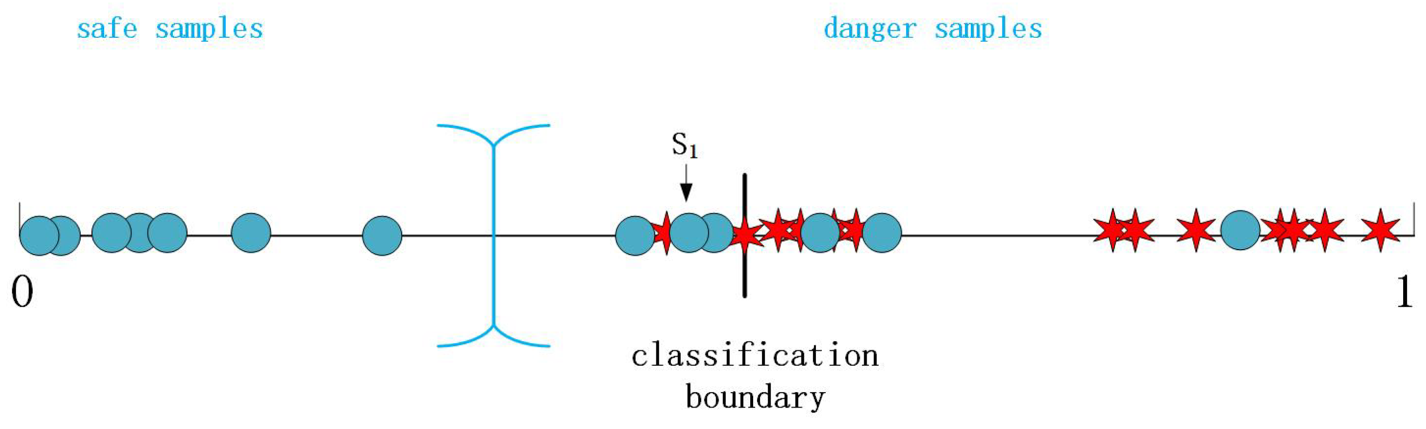
To describe the motivation of this article clearly, the two-dimensional classification problem is taken as an example. It is assumed that the classification boundary is $0.5$. At a training step, there may exist a sample whose actual value $y_i$ is much closer to the classification boundary $0.5$ than its target value 0 although it is correctly classified. As shown in Figure 2, the blue point $S_1$ is exactly classified into the category labeled 0 but the degree of belonging to Class 0 is too low. In other words, the closer it gets to the boundary, the higher the probability of being misclassified. All blue points are expected to be far away from the boundary as well as to be correctly classified. So the model should strengthen the learning on samples which are misclassified and correctly classified but close to the boundary.

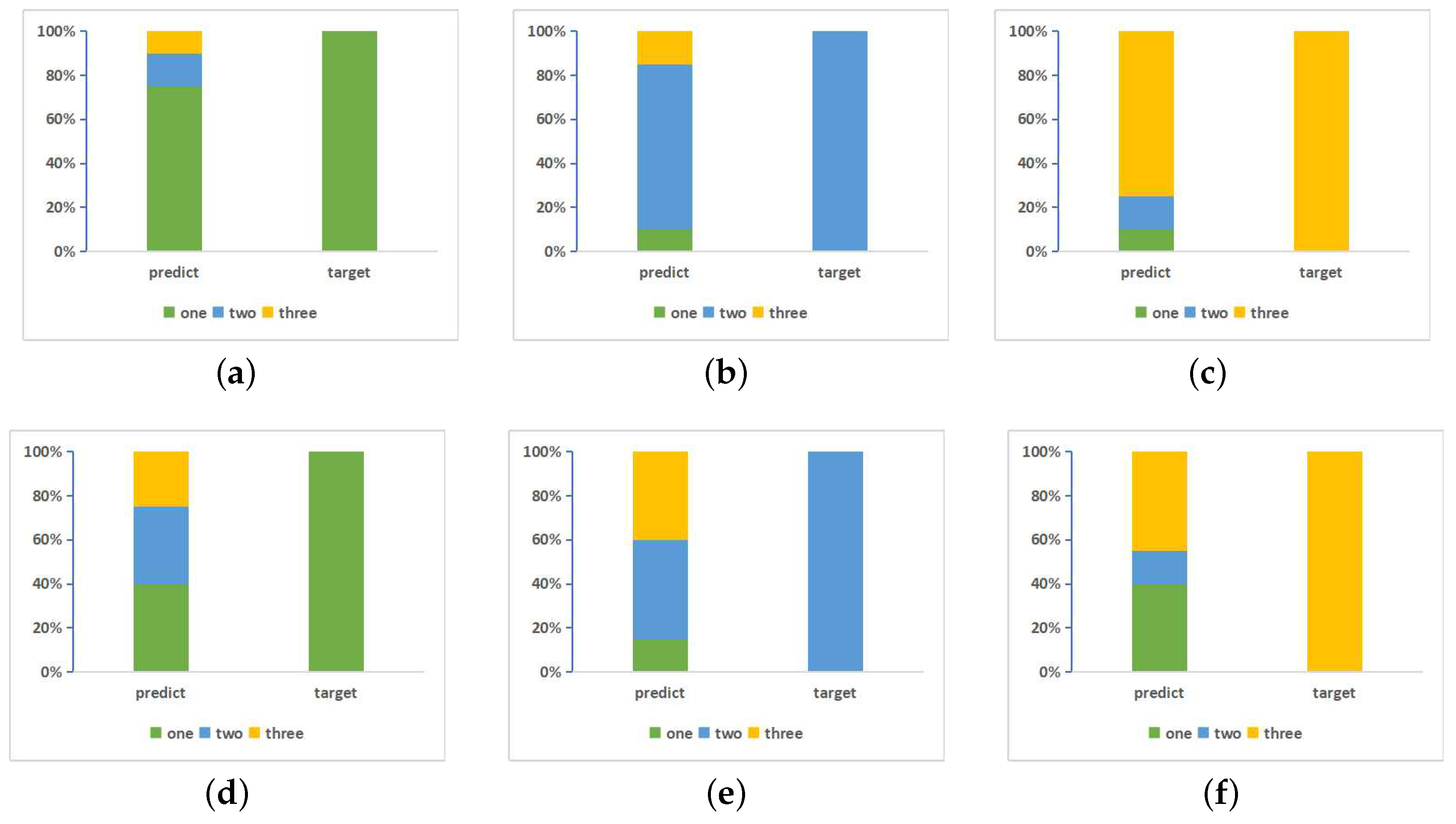
Similarly, there are also such samples in multi-class classification problems that even if they are classified into the target category, the probability with that they belong to the target category is just a bit of bigger than the probability with that they belong to other categories. As shown in Figure 3d, the right rectangle indicates that the target category of a sample is green and the areas of different colors in the left rectangle indicate the three respective output probabilities, i.e., $y_{ij}$. The biggest area is for green so that the sample is correctly classified into the green category, but the probability difference among the three colors are close to each other. In Figure 3e, the probability value of blue is just a bit greater than the yellow category. Figure 3f is similar. In Figure 3a–c, samples are explicitly and correctly classified but in Figure 3d–f, where at least two colors have similar areas, the model cannot yet fully trusted and it needs more learning.

To measure the degree to which a sample falls into its target category, this paper define a concept of the classification confidence for each sample:

$$Con{f}_i=\frac{1}{\left|t_i-y_i\right|},$$

(7)

The farther the actual value $y_i$ away from the target value $t_i$, the lower the classification confidence of the sample. The purpose of this article is to strengthen the training of samples with low confidence.

To determine which samples need to be learned strengthenly, this paper divides samples of the each category into the danger and the safe. The intuitive thinking is to set a threshold of the classification confidence for each category. If the confidence is less than the threshold, the sample is called a danger sample; otherwise, it is regarded as a safe one. However, the choice of the threshold is crucial, and its value directly affects the division of samples. If the threshold value is high, all samples may be considered as danger samples; if it is too low, all samples could be regarded as safe samples, which is similar with general ways. These situations make the network unable to focus on samples which are closed to the classification boundary. In additional, the threshold value should be different for different datasets. In summary, it is difficult and complicated in practice to determine a threshold for the confidence. A dynamic division criterion is proposed here.

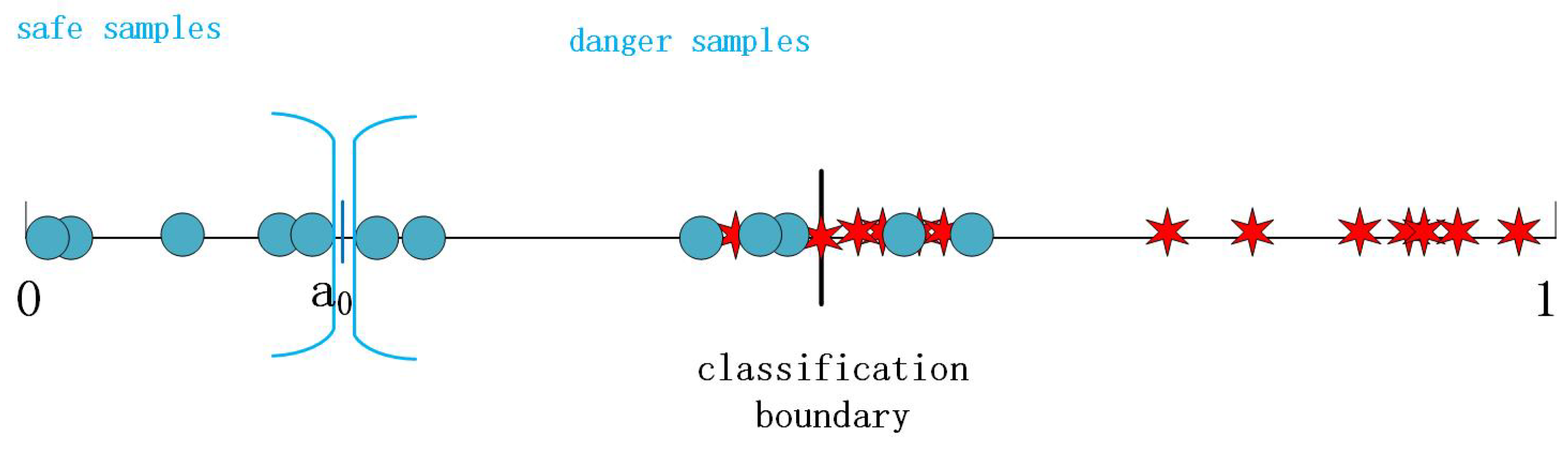
Take the two-dimensional classification problem again. Let ${\alpha }_j$ be the average actual output of all samples of the j-th class,

$${\alpha }_j=\frac{1}{r}(y_j^1+y_j^2+\cdots +y_j^r),$$

(8)

where r is the number of samples belonged to the j-th class. ${\alpha }_j$ constantly adjusts according to the actual value of all samples in this category during the training process. This article divides samples of each category into the danger and the safe such that the safe and the danger samples have high and low classification confidences, respectively, i.e.,

$$Sampl{e}_i\in \left\{\begin{array}{cc}\hfill danger,& \hfill if{(-1)}^{t_i}·({\alpha }_i-y_i)<0\\ \hfill safe,& \hfill otherwise.\end{array}\right.$$

(9)

In short, the i-th danger sample of Class 0 mean that its actual value is higher than ${\alpha }_i$, while the i-th safe sample of Class 0 indicate that its actual value is lower than ${\alpha }_i$, as shown in Figure 4.

This paper is intended to strengthen learning of danger samples by appropriately increasing the error of danger samples in the loss function, where the increased error is the difference between the classification confidence of the danger samples and the average of the classification confidence of the correct categories to which they belong. It can be realized by adding a penalty term to the loss function, so that the network strengthens the punishment of danger samples during the training process. CNN trained by this new learning algorithm is called PCNN and its detail is described with Algorithm 1. The new loss functions can be written as:

$$NMSE=\frac{1}{n}\left[(1-\lambda )·\sum _{i=1}^n{(t_i-y_i)}^2+\lambda ·\sum _{p\in danger}{({\alpha }_p-y_p)}^2\right],$$

(10)

$$NCE=-\frac{1}{n}\left[(1-\lambda )·\sum _{i=1}^n{T}_i^T·log{Y}_i+\lambda ·\sum _{p\in danger}(log{\alpha }_p-log{y}_p)\right],$$

(11)

where $\lambda$ is the proportion of the penalty term in the new loss function, NMSE and NCE refer to the modification of the original loss functions MSE and CE, respectively. If $\lambda$ = 0, the new loss functions are equivalent to the original ones. So they are the generalization of the original ones. Meanwhile, the effect of the penalty item increases with the $\lambda$ value increasing. If $\lambda$ = 1, only the penalty term exists in the new loss function. Since the value of the penalty term is small, the network can’t be trained. Therefore, $\lambda$∈ [0,1).

Algorithm 1 The new learning algorithm

Input:  Training set, learning rate, batch size. Output:  PCNN, which is the network whose weights and thresholds have been determined. 1: Set the maximum number of iteration; 2: The weights and thresholds are randomly initialized; 3: Repeat 4: Divide the training set into batches according to batch size, for each batch do: a.  Calculate the actual value for each sample of the batch according to Equations (3) or (4); b.  Calculate the average of actual values for each class based on Equation (8); c.  Find danger samples of each class according to Equation (9); d.  Calculate the loss according to Equations (10) or (11); e.  Update weights and thresholds using batch gradient descent. 5: Until   The maximum number of iteration is reached.

4. Experimental Results

In this section, the effectiveness of the new learning algorithm is verified by comparing the classification accuracy of PCNN and CNN, where PCNN and CNN respectively represent the convolutional neural network trained by the new algorithm and the traditional BP algorithm. The experiments are conducted on CIFAR-10 [24] and MNIST [25] datasets, which have been divided into the training and test sets. The architecture of CNN is designed as shown in

Table 1. The architecture of CNN.

Layer	CIFAR-10	MNIST
input	$32\times 32\times 3$	$28\times 28\times 1$
Convolution	$3\times 3\times 64$	$3\times 3\times 64$
Convolution	$3\times 3\times 64$	$3\times 3\times 64$
Max-pooling	$2\times 2$	$2\times 2$
Convolution	$3\times 3\times 128$	$3\times 3\times 128$
Convolution	$3\times 3\times 128$	$3\times 3\times 128$
Max-pooling	$2\times 2$	$2\times 2$
Convolution	$3\times 3\times 256$	$3\times 3\times 256$
Convolution	$3\times 3\times 256$	$3\times 3\times 256$
Convolution	$3\times 3\times 256$	$3\times 3\times 256$
Full connection + dropout	1024	1024
Output	1	10

. The size of the convolution filter is set as $3\times 3$, which can appropriately reduce the parameters of the network. Max-pooling is adopted over a $2\times 2$ pixel window with stride of 2. The activation function uses the ReLU function [12]. The Dropout method [7] is adopted in the fully connected layer to avoid over-fitting, where the keeping probability in the training set and test set are 0.5 and 1, respectively. Batch gradient descent [26] is commonly used to adjust the weights and thresholds of the network, where the batch size is chosen as 50, the learning rate is set as 0.001.

Whether PCNN or CNN, the settings of the above parameters are the same. Meanwhile, in order to avoid accidental experimental results, each experiment is repeated for 5 times with different initial random and their mean value is taken as the final result. Since the CIFAR-10 and MNIST datasets themselves have a fixed partition of the training and test set, the training/test splits are the same during the five runs. It is sufficient to repeat each experiment 5 times because the difference in classification accuracy obtained from 5 trials is small in actual experiments. The Wilcoxon signed ranks test [27] is also used to test if the results are due to chance or are the differences statistically significant. To explore the relationship between the classification accuracy of the network and the penalty proportion $\lambda$, this paper plots the variation of the classification accuracy with $\lambda$ when samples of each dataset are trained once, as shown in Figure 5. It can be seen that all accuracy curves increase with increasing of $\lambda$. The reason for this phenomenon is that the value of the penalty term (the difference between the confidence of danger samples and the average confidence of the correct category which danger samples belong to) is relatively small. So $\lambda$ chooses 0.9 to achieve better results in all experiments.

4.1. CIFAR-10

The CIFAR-10 dataset [24] consists of 60,000 images, each of which is a $32\times 32$ color map. This dataset is divided into 10 classes (airplane, automobile, bird, cat, deer, dog, frog, horse, ship and truck), each class contains 5000 training samples and 1000 test samples. The division of training set and test set has been fixed by the collector. In these experiments, three binary sub-datasets from the CIFAR-10 dataset are constructed, where the airplane and automobile classes form the first sub-dataset, the deer and horse classes make up the second sub-dataset, the ship and truck classes constitute the third sub-dataset. In these datasets, Equation (10) is used as the loss function. Finally, PCNN is implemented on these sub-datasets, and its classification results are compared with those of the traditional CNN and CNN with $L_2$ regularization, respectively.

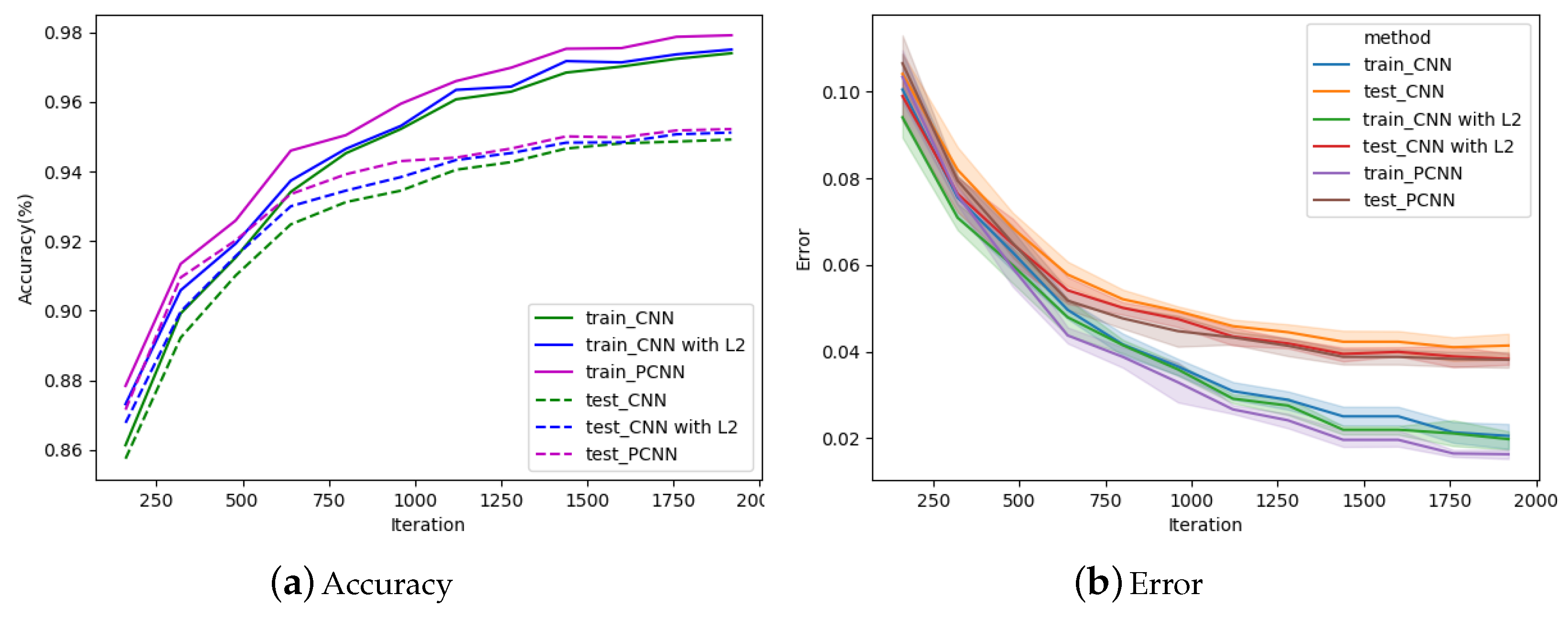
Figure 6 shows the experimental results of PCNN, CNN and CNN with $L_2$ regularization at different iterations on the first sub-dataset (airplane vs. automobile). It can be seen from Figure 6a that whether on PCNN, CNN or CNN with $L_2$, the classification accuracy increased with the increase of the number of iteration. When the number of iteration is 1920, the test accuracy of CNN achieves 96.15%, CNN with $L_2$ reaches 96.3%, while PCNN achieves 96.44%. The performance of PCNN is better than others in the whole process, especially when the number of itreation is less than 1280. If the number of iteration is 640, the test accuracy of PCNN is 1.25% higher than that of CNN. To verify if there is a statistically significant difference in test accuracies between CNN and PCNN, the Wilcoxon signed ranks test is adopted. The five test accuracy values obtained by CNN and PCNN respectively in the last iteration are recorded as two groups. The results of the Wilcoxon signed ranks test on the two groups of the first sub-dataset (airplane vs. automobile) are shown in

Table 2. The results of the Wilcoxon signed ranks test.

	PCNN-CNN
Dateset	Airplane vs. Automobile	Deer vs. Horse	Ship vs. Truck	Mnist
Z	${-2.0889}^a$	${-1.9845}^a$	${-2.1934}^a$	${-2.6112}^a$
$Asymp.Sig.(2-tailed)$	$0.0367$	$0.0472$	$0.02828$	$0.009$

[a.] Based on positive ranks.

. It can be seen that the $Sig.$ value is 0.0367, which is less than 0.05, indicating that there is a statistically significant difference (the null hypothesis H0 is rejected). Hence, the test accuracy of PCNN is improved compared with the original CNN from the perspective of statistical analysis.

Figure 6b is to aggregate multiple measurements of training and test error values by plotting the mean and the 95% confidence interval around the mean. It can be seen from Figure 6b that the error curve of PCNN is always lower than other curves, whether it is train or test error, which effectively illustrates that PCNN makes full use of danger samples so that the network learns more accurately.

The second sub-dataset is composed of deer and horse classes. The experimental results on this sub-dataset are shown in Figure 7. Due to the high similarity between these two classes, all test accuracies do not reach 90% after 2240 iterations as shown in Figure 7a, but the classification effect of PCNN is still better than others. When iteration = 2240, the test accuracy of CNN is 88.93%, the accuracy of CNN with $L_2$ is 89.09% and that of PCNN is 89.37%. When the number of iteration is greater than 1440, all test accuracy curves begin as slow grades. The curves of PCNN stays at the top. Then, the Wilcoxon signed ranks test is used to verify that the performance of PCNN is better than CNN. The two groups of the second sub-dataset (deer vs. horse) are respectively composed of five test accuracy values obtained by CNN and PCNN in the last iteration. As shown in Table 2, the $Sig.$ value obtained by the Wilcoxon signed ranks test is 0.0472, less than 0.05, indicating that there is a statistical difference in the test accuracy. Figure 7b reflects the variation of the error with the number of iterations. When the iteration is greater than 1440, the test and train error of PCNN are both lower than others, indicating that samples are not only correctly classified but also far from the classification boundary.

Figure 8a indicates the classification accuracy curves for PCNN, CNN and CNN with $L_2$ on the third sub-dataset (ship vs. truck). It shows that PCNN has better classification performance at any iterations than others, especially the number of iterations is less than 1120. After 1920 iterations, the test accuracy of CNN and CNN with $L_2$ reach 94.92% and 95.12%, respectively, and the test accuracy of PCNN reaches 95.22%. Compared to CNN, the improvement of PCNN varies from period to period, with values ranging from 0.17% to 1.73%. Then, the Wilcoxon signed ranks test is used to test the two groups composed by five test accuracy values obtained by CNN and PCNN in the last iteration. It can be seen from Table 2 that the $Sig.$ value is 0.02828, less than 0.05, proving that there exists a statistically significant difference and that the classification performance of PCNN is better than CNN in the third sub-dataset (ship vs. truck). Figure 8b shows the errors of PCNN, CNN and CNN with $L_2$ during the training process, and the errors gradually decrease with the increase of the number of iterations. After 1920 iterations, the test errors of CNN and CNN with $L_2$ decrease to 4.14% and 3.83%, respectively, while the test error of PCNN decreased to 3.816%.

4.2. MNIST

MNIST [25] is a dataset for the study of handwritten numeral recognition, which is component of 55,000 training samples and 10,000 test samples. The collector of this dataset has determined the partitioning of the training and test sets. Each sample is a $28\times 28$ gray image. This dataset is divided into 10 classes, representing 0 to 9, respectively. In this experiment, Equation (11) is taken as the loss function, and the impact of PCNN on the multi-class classification problem is explored.

Experiments are carried on CNN, CNN with $L_2$ and PCNN under different iterations The results are illustrated in Figure 9. As can be seen from Figure 9a, when the number of iteration is less than 5500, the test accuracy of PCNN is significantly higher than that of CNN and CNN with $L_2$. At 8800 iterations, the test accuracy of CNN and CNN with $L_2$ are 99.246% and 99.274%, respectively, while that of PCNN is 99.3%. Similarly, the Wilcoxon signed ranks test is used to test whether there is a statistically significant difference in the classification accuracy of PCNN and CNN on MNIST dataset. As shown in Table 2, the $Sig.$ value is 0.009, which is less than 0.05, indicating that PCNN can indeed improve classification accuracy from statistical analysis.

Table 3. The comparison of classification results on MNIST.

Method	Test Accuracy (%)
$PCNN\left[ours\right]$	$99.3$
$Versatile-Model3$ [28]	$99.22$
$Graph-CNN$ [29]	$99.14$
$CNNMA$ [30]	$98.75$
$MCNN-DS$ [31]	$98.43$

shows test accuracy on PCNN and other algorithms. Obviously, the new learning algorithm proposed in this paper is better than other algorithms. In Figure 9b, the train error and test error of PCNN are lower than others in the whole process. After 8800 iterations, the test error of CNN, CNN with $L_2$ and PCNN reaches 2.84%, 2.77%, and 2.65%, respectively.

5. Conclusions

This paper proposes a new learning algorithm to improve the classification performance of CNNs. The new algorithm focuses on the gap between the average classification confidence of a category and the respective classification confidence of danger samples of the same category. It strengthens the training of danger samples which have low classification confidence by penalizing the loss function with danger samples. Meanwhile, the new loss function can be seen as the generalization of the old loss function. The experimental results on the three sub-datasets of CIFAR-10 and MNIST dataset indicate that the proposed learning algorithm can improve the classification performance of CNN, whether in the two-class or multi-class classification problem. In future research, the weight $\lambda$ of penalty item is attempted to be set as dynamic parameter, so that it can automatically adjust according to the classification accuracy of the whole samples in network training, thus speeding up network training and improving classification accuracy.