Abstract
The Integrated Gasification Combined Cycle (IGCC) possesses a number of advantages over traditional power generation plants, including increased efficiency, flex-fuel, and carbon capture. A lesser-known advantage of the IGCC system is the ability to coordinate with the smart grid. The idea is that process modifications can enable dispatch capabilities in the sense of shifting power production away from periods of low electricity price to periods of high price and thus generate greater revenue. The work begins with a demonstration of Economic Model Predictive Control (EMPC) as a strategy to determine the dispatch policy by directly pursuing the objective of maximizing plant revenue. However, the numeric nature of EMPC creates an inherent limitation when it comes to process design. Thus, Economic Linear Optimal Control (ELOC) is proposed as a surrogate for EMPC in the formulation of the integrated design and control problem for IGCC power plants with smart grid coordination.
1. Introduction
Compared to traditional power plants, Integrated Gasification Combined Cycle (IGCC) based power plants have many advantages including increased efficiency, flex-fuel, and carbon capture opportunities. A conventional IGCC power plant can be described by Figure 1, if the methanol plant and storage units are removed. In the gasification block, coal and oxygen are converted into synthesis gas, which is subsequently cleaned and decarbonized to produce a stream of nearly pure hydrogen. This stream of hydrogen is then sent into the power block to generate electricity. A portion of the generated electricity is consumed by the compressors for air separation and carbon dioxide sequestration operations.
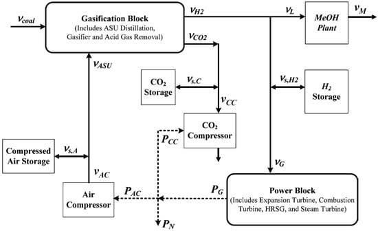
Figure 1.
Simplified diagram of an IGCC power plant with equipment upgrades for power dispatch. ASU, Air Separation Unit.
The IGCC plant can be modified to achieve smart grid coordination [1] through power output dispatch. The modified IGCC plant can adjust its electricity output to track grid demand and thus take advantage of electricity price fluctuations. The ability to change electricity output from an IGCC plant can be obtained by a variety of hardware configurations. The most common cited configuration is poly generation, in which a portion of the hydrogen stream generated from the gasification block is diverted elsewhere during periods of low electricity price. This diverted hydrogen could be chemically converted to a liquid fuel (possible methanol) or sold directly [2]. The hydrogen can also be put into storage during periods of low electricity price and then drawn from the storage during peak electricity demands (high electricity price periods). Similarly, regarding the Air Separation Unit (ASU), a compressed air storage unit can be placed between the air compressor and the cryogenic distillation units. This configuration would maintain a constant flow of compressed air to the cryogenic distillation, while allowing the power consumed by the air compressors to be anti-related with the electricity price, which would increase the net power output of the IGCC plant during high price periods. By the same token, a carbon dioxide storage unit can be added, so that part of the captured carbon dioxide can be stored at an intermediate pressure during periods of high electricity price and eventually pressurized during low-price periods. It should be noted that an unmodified IGCC plant also has dispatch capabilities, owing to the fact that the gasification block can change hydrogen production rates. However, due to the slow response time of the cryogenic distillation portion of the ASU, the ramp rate of the gasification block is quite slow [3].
A fundamental question for smart grid coordination is the development of a control structure capable of employing information from the smart grid. The first issue is about regulatory control, i.e., set-point tracking abilities and ramping capabilities. Several efforts have investigated this issue for a variety of IGCC configurations, as well as specific unit operations [2,3,4,5]. While regulatory controller design is important, such efforts typically lack sufficient motivation, because the performance objectives of the desired set-point ranges and achievable ramp rates are set somewhat arbitrarily. Thus, to arrive at sufficient motivation, one must consider supervisory control, which will determine the set-points for the regulatory control.
One approach to define a supervisory controller is to set the goal to be maximization of average revenue, which equals the integral of the product of electricity price and net power produced. The electricity price signal would be an input to the controller. However, unlike a disturbance, the objective is not to minimize its impact on the output. This supervisory control problem can be addressed using Economic Model Predictive Control (EMPC) [6]. Specifically, the typical quadratic objective function in MPC [7] will be replaced by an expression directly reflecting the revenue. Similar approaches have been applied to the area of Heating, Ventilation, and Air Conditioning (HVAC) control [8,9,10,11], the area of process operations scheduling [12,13,14,15,16,17,18,19,20], as well as the area of electric power system operations [21,22,23,24]. As mentioned above, the power dispatch capability of an IGCC plant can be achieved by a variety of hardware configurations. While EMPC works well for process control, it has limitations when it comes to system design. Specifically, it cannot handle binary variables, which indicate the attendance of specific hardware units. To overcome this limitation, Economic Linear Optimal Control (ELOC) based process design is proposed. ELOC is a recently established control strategy that combines process control and process economics [25,26,27,28], and its control policy has been shown to yield an economic performance similar to a large horizon EMPC policy for HVAC system [29], as well as for a simplified IGCC power dispatch system [16]. ELOC based process design has been proposed for building HVAC systems [30] and electric power networks [31,32]. In addition, a preliminary version of ELOC based process design for IGCC plants was provided in [33]. However, the approach provided in [33] cannot handle binary variables in the design problem.
The structure of the paper is as follows. Section 2 introduces the model of electricity price and the model of the IGCC plant with power dispatch and illustrates the ability of EMPC to maximize revenue on a variety of hardware configurations. Section 3 introduces ELOC and shows that ELOC results in a control policy similar to EMPC. In Section 4, ELOC will be extended to the integrated control and design problem.
2. IGCC Power Dispatch System Model and EMPC
Electricity price fluctuations are fundamental to this study and are the primary motivation to develop the IGCC power dispatch system. Subsequent to the establishment of the electricity price model and the dispatch capable IGCC system model, EMPC will be introduced, and its ability to maximize the revenue will be illustrated through examples of the IGCC system with different configurations.
2.1. The Model of Electricity Price
The price of electricity () is known to have an oscillatory characteristic of a period of one day. It can be simply modeled as a sinusoidal function for rough analysis. Meanwhile, it can also be modeled as a third order shaping filter to achieve a much more realistic representation. In the latter case, the electricity price can be modeled by the following third order shaping filter [33]:
where , h, , h, is a (to be determined) design parameter, w is a Gaussian, zero-mean white noise process with spectral density:
and is the variance of the electricity price.
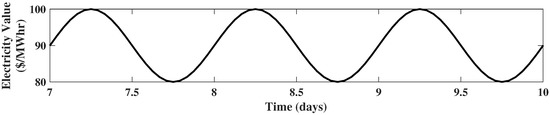
The reason for the use of this third order shaping filter is that we know electricity price possesses an oscillatory characteristic of one day, and thus, it can be modeled as the output of an underdamped second order system driven by white noise. However, such a model may allow too much of the low-frequency energy contained in the white noise to pass through to . Thus, a high pass filter is added to the white noise to remove its low frequency components, which results in the above third order shaping filter. In addition, an important idea about this shaping filter is that, for all parameter values (, , , , and ), the calculated variance of through a stochastic covariance analysis of Equation (4) is always equal to . If we set $, $/(MW h), and $/, a realization of generated from (4) is given in Figure 2.
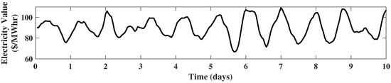
Figure 2.
A realization of the stochastic process used to model electricity prices.
2.2. The Model of the IGCC Power Dispatch System
The process diagram of Figure 1 illustrates the proposed process modifications. The compressed air storage unit (added between the air compressor and the ASU in the gasification block) allows for independent manipulation of and (mass flows of compressed air from the air compressor and to the ASU, respectively) by setting the difference equal to (the mass flow to the storage unit). The amount of mass in the air storage unit, , is simply the time integral of . The hydrogen storage unit and methanol synthesis reactor system (added between the gasification and power generation block) allow for independent manipulation of , , and (mass flows of hydrogen from the gasification block, to the methanol synthesis reactor system, and to the power block, respectively). By setting (the mass flow to the storage unit), the amount of mass in the hydrogen storage, , is simply the time integral of . The carbon dioxide storage added between the gasification block and carbon dioxide compressor allows for independent manipulation of and (mass flows of carbon dioxide from the gasification block and to the carbon dioxide compressor, respectively). By setting the difference equal to (the mass flow to the storage unit), the amount of mass in the carbon dioxide storage unit, , is simply the time integral of . The relation between power and mass flow to the air compressor is assumed to be linear ; the relation between mass flows of compressed air and coal to the gasification block is assumed to be ; the relation between mass flows of coal to the gasification block and hydrogen production is assumed to ; the relation between hydrogen mass flow to power block and generated power is assumed to be ; the relation between hydrogen mass flow to the methanol synthesis reactor system and methanol production is assumed to be ; the relation between carbon dioxide production and the mass flow of coal to gasification block is assumed to be ; the relation between the mass flow of compressed carbon dioxide and power to the carbon dioxide compressor is assumed to be . Finally, the net power generated for the grid is calculated as a simple power balance: . Converting the above model description into a state-space model yields:
The operating constraints that reflect physical realities and capacity limitations of assumed equipment are as follows:
The following relations can be obtained through a time-average analysis of (6): , , and , where , , , , and are the time-averaged values of , , , , and , respectively. There is no limitations imposed by time-average analysis of (6) on the average mass within the storage. Therefore, we select , , and .
By defining the process state, manipulated, and performance variables as , and , respectively, the system (6) and (7) can be written in the following form:
where:
If the data of Case B1B: Shell IGCC Power Plant with Capture from the NETLBaseline Report [34] are used (see Table 1 and Table 2), the model parameters can be determined, and their values are shown in Table 3. The parameter is obtained based on a methanol synthesis reaction using carbon dioxide and hydrogen as reactants.

Table 1.
Case B1B stream table.
Table 2.
Case B1B plant performance.
Table 3.
The values of parameter .
Regarding the bounds on q, will be treated as a vector of parameters throughout the paper; will be treated differently depending on the type of optimization problem. In an optimal control problem (Section 2.3 and Section 3), will be treated as a parameter vector with fixed values. In contrast, in the integrated design and control problem (Section 4), will become a vector of variables except for its element . The element will always have a fixed value, since we assume that the maximum coal flow rate to the gasification block cannot be increased. With being a vector of variables, its value changes represent the changes to equipment size.
2.3. Economic Model Predictive Control
Consider a process model: , , where s, m, p, and q are state manipulated, disturbance, and performance output vectors, respectively. The process constraints on the performance outputs are . To implement Model Predictive Control (MPC), the continuous-time model must be converted into discrete-time form. Then, combined with the notion of a predictive time index and economic objective function, the MPC problem is obtained as:
where the index i represents the actual time of the process and index k is the predictive time. The idea of MPC is that given an estimate of initial condition, , at a time i, and the forecast of disturbances , a sequence of control actions, , can be determined by solving the problem (13). However, only the first control action is used as the input, , to the process . Then, at the next time step, the new initial condition and new disturbance are estimated based on new measurements. For additional information on MPC, please see [7].
The only difference between Economic MPC (EMPC) and traditional MPC is the objective function. In traditional MPC, a quadratic objective function is used to track a pre-determined setpoint for process operation, whereas in EMPC, the quadratic objective function is replaced by the operating cost of the process, . In many cases, the function is a simple linear function, which has no minimum. Thus, the constraints are crucial in order to generate a meaningful controller. For additional information on EMPC, please see [6,17,18].
In the EMPC implementation, forecasts of electricity price will be needed. However, to focus on the fundamental issues, this paper will assume the forecast to be perfect, in the sense that they are error free and do not change with time. As such, the “hat” notation in the EMPC formulation will be dropped. This assumption has been shown to be not critical in the evaluation of EMPC in [16], which investigated EMPC for a simple IGCC power dispatch system with both perfect and imperfect forecasts. For additional information on forecasting, see [11]. The IGCC plant model developed in Section 2.2 will be converted to discrete-time form for EMPC implementation, using the sample and hold method (, and ) [35] with a sample time of h. Regarding the objective function, denotes electricity price during period i; is the price of methanol; is the cost of coal; the revenue during period i is . Thus, the formulation of the EMPC problem for IGCC dispatch is:
where the objective function denotes the average revenue per period . Clearly, the problem (18) can be solved using a standard linear programming solver. It should be noted that the final cost term is not included in the problem (18). This term is essential to guarantee stability for short horizon EMPC (see [6,18]). However, for the current application and with the given horizon, this term plays a less important role and is omitted due to space constraints.
Five examples will be provided to illustrate the ability of EMPC to maximize the revenue for an IGCC power plant with dispatch. For the sake of clarity, the first four examples with increasing complexity of upgrades will use a sinusoidal function to represent the electricity price, whereas the fifth example with fully developed upgrades will employ the shaping filter introduced in Section 2.1 as the model of electricity price. The corresponding process model for each example can be obtained by proper modification of the IGCC model proposed in Section 2.2. In addition, the EMPC implemented in all the examples will have a prediction horizon of 24 h with a sample time of 1 h.
Example 1.
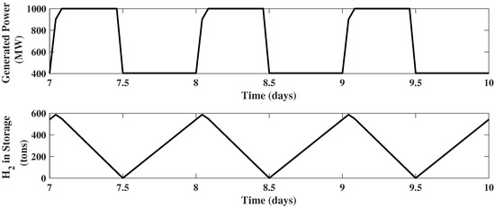
IGCC plant with only hydrogen storage: The operating conditions of Case B1B of the NETL Baseline Report [34] serve as the basis of all examples. Specifically, the conditions for the IGCC power plant without dispatch are: MW, MW, MW, tons coal/h, tons /h, tons compressed air/h, tons /h, and /ton coal. For the current example, assume only two upgrades are performed. The first is to add a hydrogen storage unit with a capacity of 600 tons ; the second is to increase the size of power block, so that its maximum output is 1000 MW. Moreover, assume that only these two units are capable of dynamic operation and all other units remain at nominal operating conditions. In this case, the state variable is the mass of hydrogen in the storage, , and the manipulated variable is the power generated, . The bounds on the process variables are assumed to be ton , tons , MW (60% of ), and MW.
In this scenario, the results of the EMPC using a 24 h prediction horizon are shown in Figure 3. As expected, the manipulated variable, , is at its maximum when the electricity price is high and at its minimum when electricity price is low. The hydrogen storage is filled up during the low electricity value periods and gets discharged during high electricity value intervals.
Figure 3.
Closed-loop simulation of Economic Model Predictive Control (EMPC) using a 24 h prediction horizon for Example 1.
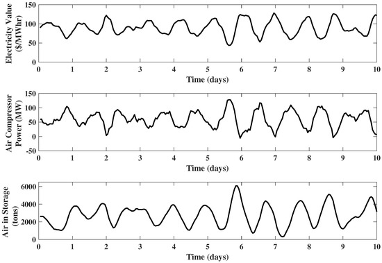
Example 2.
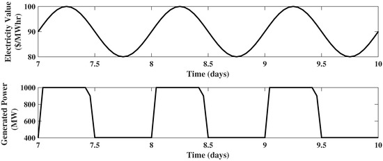
IGCC plant with hydrogen storage and compressed air storage: Reconsider the IGCC system of Example 1. Now, in addition to hydrogen storage and power block expansion, two additional upgrades are performed. The first is to add a compressed air storage unit with a capacity of 3000 tons of compressed air; the second is to upgrade the power capacity of the air compressor to 200 MW. In this case, five units are capable of dynamic operations: hydrogen storage, the power block, the air compressor, compressed air storage, and the gasification block ( now assumed to be adjustable). The state variables are , and the manipulated variables are . Regarding the process constraints, ton compressed air, tons compressed air, MW, MW, tons coal/h (60% of ), and tons coal/h.
The results of the EMPC using a 24 h prediction horizon are shown in Figure 4. It is observed that the plots of generated power and hydrogen in storage are quite similar to Example 1. However, the behavior of air compressor is opposite to the power generator. This is because unlike the power generator, which produces electricity, the air compressor consumes electricity. Thus, the electricity consumed by the air compressor increases to its maximum when the electricity price is low and is at its minimum when electricity price is high. The periods at which is at the nominal value ( MW) correspond to intervals in which the compressed air storage is full and the energy value is increasing or the compressed air storage is at its minimum and the energy value is decreasing. This behavior is due to the fact that the controller has no other reasonable option under these conditions, since the production of hydrogen is maintained at its maximum all the time.
Figure 4.
Closed-loop simulation of EMPC using a 24 h prediction horizon for Example 2.
Example 3.
IGCC plant with hydrogen, compressed air and carbon dioxide storages: Assume another two new upgrades are made on the IGCC system of Example 2. The first is to add a carbon dioxide storage unit with a capacity of 2000 tons carbon dioxide; the second is to upgrade the power capacity of carbon dioxide compressor to 100 MW. Then, the state variables become , and the manipulated variables are . In addition to the bounds of Example 2, we also require ton , tons , MW, and MW.
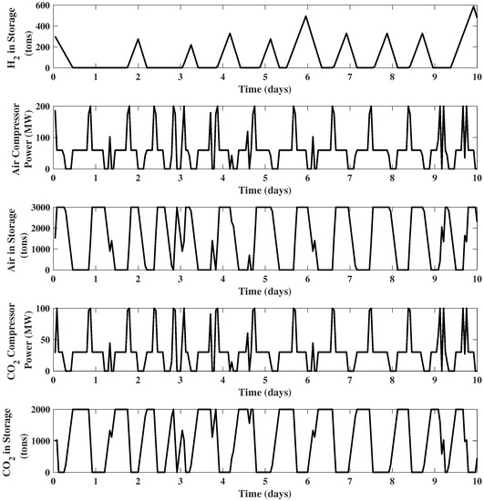
The results of the EMPC using a 24 h prediction horizon are shown in Figure 5. The plots for compressed air storage , hydrogen storage , power consumed by air compressor , generated power , and coal flow rate are omitted, since all of them remain the same as Example 2.
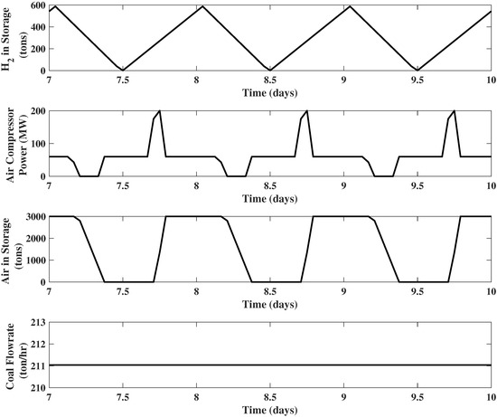
Figure 5.
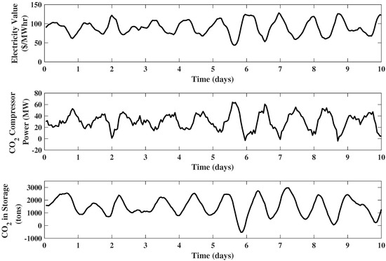
Closed-loop simulation of EMPC using a 24 h prediction horizon for Example 3.
Although the carbon dioxide compressor operates at its nominal value ( MW) during the majority of the time, when the electricity price is high, the power consumed by the carbon dioxide compressor will drop to and stay at zero, which means the compressor will be turned off. When the electricity price is low, the carbon dioxide compressor will increase its power consumption to compress more carbon dioxide from the storage. As a result, the storage of carbon dioxide will be fully discharged. This behavior is quite opposite to the compressed air storage. The reason is that unlike the compressed air storage (placed after the air compressor), the carbon dioxide storage is placed before the compressor. During high electricity price periods, the carbon dioxide compressor is turned off, and the carbon dioxide generated from the gasification block will be sent into storage. Then, when electricity price becomes low, and the carbon dioxide coming from both the gasification block and carbon dioxide storage will be compressed.
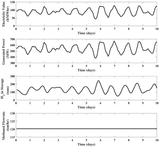
Example 4.

IGCC plant with hydrogen, compressed air, and carbon dioxide storages, as well as a methanol plant: Reconsider the IGCC system of Example 3. Now assume there is another option for the hydrogen stream produced from the gasification block: it can be sent to a methanol synthesis reactor system. The bounds on the methanol production rate are assumed to be ton MeOH/h and tons MeOH/h. Obviously, the price of methanol will directly determine whether it is worth sending the hydrogen to the methanol synthesis reactor. Thus, three cases with different methanol prices are investigated. In all cases, only the plots of methanol flow rate , generated power , and hydrogen in storage will be presented, since the production of hydrogen is always maintained at its maximum, and thus adding the option of methanol production will not affect the optimal operation of other components of IGCC plant, except for power generation and hydrogen storage.
If the selling price of methanol is 100 $/ton, it turns out that no hydrogen is sent to the methanol synthesis reactor system. The reason is that for this price, less revenue will be obtained by selling methanol than selling electricity.
If the price of methanol is increased to 150 $/ton, it is found that now, most of hydrogen is sent to the methanol synthesis reactor, and the power generation stays at its minimum value. This behavior indicates that with this methanol price, it apparently generates more revenue by producing methanol than producing electricity.
Finally, if the selling price of methanol is 110 $/ton, both plants take part in production, as shown in Figure 6. It can be observed that the generated power possesses a behavior similar to previous examples, working at its maximum capacity when the electricity price is high and at its minimum when the electricity price is low. The methanol production reaches a high level when the electricity price is low and drops to zero when the electricity price is high.
Figure 6.
Closed-loop simulation of EMPC using a 24 h prediction horizon for the case of $/ton MeOH for Example 4.
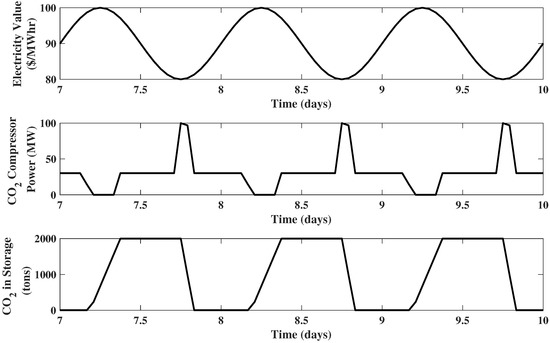
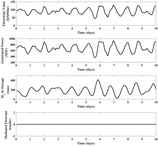
Example 5.
IGCC plant with full upgrades and electricity modeled with the shaping filter: Reconsider the IGCC system of Example 4. Now, assume the electricity price is modeled by the third order shaping filter introduced in Section 2.1 with $, $/(MW h), and $/. The methanol price is set to 110 $/ton.
The results of the EMPC are illustrated in Figure 7. It is observed that the electricity price no longer evolves uniformly, and a more realistic performance of the system variables is obtained.
Figure 7.
Closed-loop simulation of EMPC using a 24 h prediction horizon for Example 5.
2.4. The Impact of Storage Size
Naturally, it is expected that different storage sizes will result in different optimal control policy. In this subsection, the impact of compressed air storage size, carbon dioxide storage size, and hydrogen storage size will be illustrated through three examples, respectively. All examples use a prediction horizon of 24 h when implementing the EMPC.
Example 6.
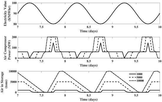
Reconsider the IGCC system of Example 2. Three cases are studied, each assuming the size of the compressed air storage to be 1000 tons, 5000 tons, and 10,000 tons, respectively. All the other information about the IGCC system remains the same as Example 2.
Comparison of these three cases is illustrated in Figure 8. In all cases, the plots for generated power , hydrogen in storage , and coal flow rate are the same as Example 2 and thus omitted for simplicity. From Figure 8, it is observed that as the compressed air storage size increases, the air compressor will be kept turned off for a longer time when the electricity price is high and will be at its maximum capacity for a longer time when the electricity price is low. Thus, overall, larger compressed air storage will result in better economic performance. This conclusion is supported by the following data: the 10 day revenue obtained from EMPC for these three cases (compressed air storage size being 1000 tons, 5000 tons, and 10000 tons) is $, $, and $, respectively.
Figure 8.
Closed-loop simulation of EMPC using a 24 h prediction horizon for Example 6.
Example 7.
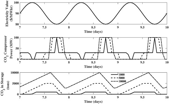
Reconsider the IGCC system of Example 3, but assume the size of the carbon dioxide storage to be 1000 tons, 5000 tons, and 10,000 tons, respectively. All the other information about the hardware of IGCC systems remains unchanged.
In all cases, the plots for generated power , power consumed by air compressor , hydrogen in storage , compressed air in storage , and coal flow rate are the same as Example 3. From Figure 9, a similar behavior is observed: as the carbon dioxide storage increases, the carbon dioxide compressor will be kept turned off for a longer time when the electricity price is high and will be at its maximum capacity for a longer time when the electricity price is low. The 10 day revenue obtained from EMPC for these three cases (carbon dioxide storage size being 1000 tons, 5000 tons, and 10,000 tons) are $, $, and $, respectively.
Figure 9.
Closed-loop simulation of EMPC using a 24 h prediction horizon for Example 7.
It should be noted that in the 10,000 ton case, the storage is not being fully utilized. Specifically, the storage is never completely emptied, suggesting that the exact same revenue could be achieved with a smaller storage, say 6000 tons. We will see a similar result in the next example.
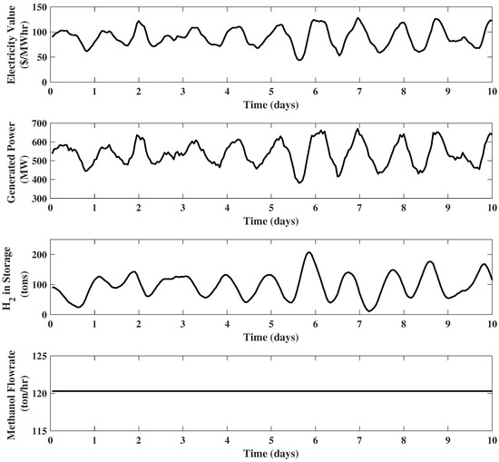
Example 8.
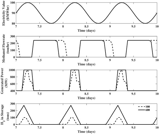
Reconsider the IGCC system of Example 4 with methanol price $/ton MeOH. Now, reduce the hydrogen storage size to 100 tons. All the other information about the IGCC system remains unchanged. From Figure 10, it can be seen that when the hydrogen storage size is reduced to 100 tons, the generated power will stay at its maximum for a much shorter time during the high electricity price periods. Meanwhile, the methanol production will maintain at a high level for a much longer time, and more methanol will be produced. The 10 day revenue obtained from EMPC optimization for these two cases (hydrogen storage size being 100 tons and 600 tons) is $ and $, respectively.
Figure 10.
Closed-loop simulation of EMPC using a 24 h prediction horizon for Example 8.
It should be noted that despite the fact that the storage size is 600 tons, the optimal operating policy never utilizes all of that storage. In fact, for that case, the exact same revenue would be generated with a storage of about 300 tons. However, if the price of MeOH was reduced to 100 $/ton, then Example 4 indicates all 600 tons of would be utilized.
Thus, it is clear that the equipment size can directly affect the optimal operation of the IGCC system, and larger upgrades will yield to large revenue. However, the capital cost for larger equipment will be larger as well, which naturally leads to the following question: What are the optimal sizes of the hardware units? To answer this question, it requires a net present value assessment that weighs revenue gain against the capital cost of equipment upgrades. Unfortunately, the numeric basis of EMPC indicates that it is ill equipped for use within such an optimization scheme. This is due to the fact that black box numeric simulations are required to estimate revenue as a function of hardware configuration/size. While such an approach can be used within a local search scheme, it is far from sufficient to find global solutions to the non-convex problems that will result from the envisioned IGCC hardware design problem. Therefore, Economic Linear Optimal Control (ELOC) will be proposed as a surrogate for EMPC to perform the net present value analysis. Before diving into the IGCC design problem, first we must prove that ELOC is a appropriate surrogate for EMPC.
3. Comparison of EMPC and ELOC
We now introduce the ELOC, which can generate a linear controller capable of mimicking the EMPC policy. Reconsider the EMPC objective function, and take the limit with respect to N:
The objective function becomes the long-term average revenue per period . One approach to determine the optimal control policy for this objective is to assume has the following form:
where , , and . Additionally, , . Equation (27) indicates the basic notion that the net power production should be large when the electricity price is high and low when electricity price is low. The coefficient , yet to be determined, will indicate the magnitude of this relationship. With all these definitions, Equation (26) can be evaluated as:
where is the variance of the electricity price. Specifically, . Furthermore, , where , , and . Thus, for a given characterization of , one could optimize over , , , , , and . The characterization of is achieved by the third order shaping filter proposed in Section 2.1.
From (4), it can be seen that . Thus, to enforce an approximation of condition (27), one could require:
where is a sufficiently small parameter, but not so small that numerical infeasibility occurs ( is set to 0.01 for all cases).
The next step is to recast the compound system into deviation variable form:
Then, the compound process model (augmented with shaping filter) can be written as:
where
The continuous-time model can be converted to a discrete form using the sample and hold method (, , , and ) [35]:
The ELOC controller is assumed to be a linear feedback of the state: (Actually the controller should be where is the estimated state. The development of this partial state information case is a simple extension of the full state information case presented here; see [29] for details.). Given a candidate controller, L, the variance of the performance variable, , is calculated as:
where the vector is the row of an identity matrix and is the positive definite solution to (46). Rather than enforce the point-wise-in-time constraints, , the ELOC method follows a pseudo- (or chance-)constrained approach by enforcing the following statistical constraints:
The next step is to find a feedback controller, L, to maximize the average revenue defined by Equation (28). This controller can be determined by the following nonlinear optimization problem:
Problem (48) can be converted to a convex form by using the following theorem (a slight generalization of Theorem 6.1 from [25]).
Theorem 1.
There exists stabilizing controller L,, and , such that:
if and only if there exists, Y, andsuch that:
and:
It should be pointed out that the only difference between Theorem 1 and Theorem 6.1 in [25] is the adding of variable in (54) and (57). Using the Schur complementary theorem, LMI(57) can be easily converted to the format similar to its counterpart in Theorem 6.1 in Theorem 1. If the variable is set to one, then Theorem 1 will be reduced to Theorem 6.1 in [25].
Application of Theorem 1 to the problem (48) results in the following convex optimization problem:
Problem (60) possesses a structure similar to the ELOC problem proposed in [28] and thus can be solved globally using the same generalized Benders decomposition approach. Specifically, the complicating variables should be selected as , , and the constraint set for complicating variables consists of (61), (62), and (66). The non-complicating variables are selected as , X, Y, , and the corresponding constraint set consists of (63) and (64). Finally, the connecting constraints must be (65). Clearly, the connecting constraints are convex in the non-complicating variables. In addition, both the objective function and the connecting constraints are convex in the non-complicating variables. Thus, the GBDapproach is guaranteed to arrive at a global solution. See [36,37] for more details on GBD theory and implementation.
If and are from the solution to Problem (60), then is the solution to Problem (48), within the accuracy of the inequality constraints of Problem (60). To obtain the ELOC policy, the solution must be scaled with respect to . Specifically, the columns of corresponding to the shaping filter states must be multiplied by . This rescaling will make the control policy proper for an electricity price described by (4) with set equal to one.
Example 9.
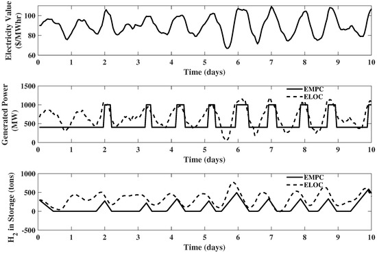
Reconsider the IGCC system of Example 5 with electricity price modeled by the same third order shaping filter. The methanol price remains unchanged. Now, we can recast the optimal control problem into the form of Problem (60) and solve it globally. The comparison of optimal control policy between ELOC and EMPC is provide in Figure 11, Figure 12 and Figure 13.
Figure 11.
Comparison of EMPC and Economic Linear Optimal Control (ELOC) policy for Example 9: generated power and hydrogen storage.
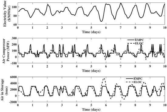
Figure 12.
Comparison of EMPC and ELOC policy for Example 9: air compressor power consumption and compressed air storage.
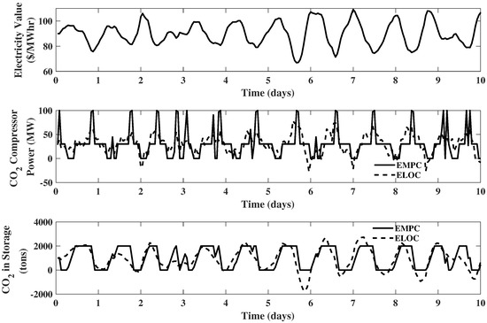
Figure 13.
Comparison of EMPC and ELOC policy for Example 9: carbon dioxide compressor power consumption and carbon dioxide storage.
It is observed that some constraint violations (power and storage levels drop below zero or go beyond upper bounds) happen in the ELOC simulation. The reason for this behavior is that the ELOC only enforces statistical constraints. Specifically, only requires that one standard deviation (68%) of the outputs will be within the lower and upper bounds. However, generally speaking, the ELOC policy controls the process variables in response to the price fluctuation in a way that is quite similar to the EMPC policy. For a quantitative comparison of EMPC and a constrained version of ELOC, please see [16,29]. Thus, ELOC is proposed as a surrogate for EMPC. In the following section, the ELOC will be used to perform net present value assessment for the IGCC dispatch system.
4. ELOC Based Integrated Design and Control of IGCC Power Dispatch System
The economic framework of the integrated design and control problem for the IGCC power dispatch system is studied in this section. We assume the existence of a steady-state based plant and consider the question of adding hardware to allow for dispatch capabilities. That is, assume the existing design specifies steady-state operating conditions as follows: , , , and . Furthermore, assume these operating conditions also specify the maximum capacity of equipment: , , . Then, the capital costs of changing the maximum capacity to , , and by adding new equipment are assumed to follow the six-tenths rule , , and , where the first term with the binary variable indicates the initial cost and the second term denotes the sizing cost. It is assumed that the capacity to process coal cannot be increased, which gives . Regarding material storage, it is assumed that the existing design does not include storage devices (, , and ). Thus, the cost of storage equipment is assumed to be , , and . Additionally, it is assumed that the existing design does not include the methanol synthesis system (). Similarly, the cost of the methanol synthesis system is assumed to be .
If no dispatch, the average revenue per time period () is defined as . From the analysis in Section 3, we know that the average revenue per time period with dispatch is . Thus, the increase in average revenue is given by
In this study, the time period is 1 h. Therefore, the present value of the increase in revenue is where:
is the annual interest rate and n is the project horizon [38]. Here, the IGCC power dispatch system is assumed to work for 326 days per year, since there is some maintenance time required each year.
Using the above analysis, we can finally state the net present value of a candidate process upgrade as:
where , , , and . The objective of the IGCC power dispatch system design is to maximize , Thus, the integrated design and control problem for the IGCC power dispatch system can be formulated by replacing the objective function in (60) with (69) and changing , , , , , , and from fixed parameters to decision variables. The result problem formulations is as follows:
s.t. (61), (62), (63), (64)
(66), (39), (40)
where the parameter with superscript appendix “ub” denotes the upper bound for the corresponding hardware. Problem (70) possesses a structure similar to the ELOC problem proposed in [28] and thus can be solved globally using the generalized Benders decomposition. Specifically, the complicating variables should be selected as , , , , , , , , , , , , , , , , and the constraint set for complicating variables consists of (61), (62), (66), (39), (40), (72), (73), (74), (75), (76). The non-complicating variables are selected as , X, Y, , and the corresponding constraint set consists of (63) and (64). Finally, the connecting constraints must be (71). Clearly, the connecting constraints are convex in the non-complicating variables. In addition, both the objective function and the connecting constraints are convex in the non-complicating variables. Thus, the GBD approach is guaranteed to arrive at a global solution. It should be pointed out that in Problem (70), statistical constraints are tightened into , which indicate that the controller obtained from Problem (70) will guarantee two standard deviations (95%) of the outputs to be within the lower and upper bounds.
Example 10.
From Case B1B of [34], it is found that the cost of the power generation block (combustion turbine, HRSG, and steam turbine) is $300,000,000; the cost of the air compressor is $125,000,000 (assumed to be half of the ASU cost); the cost of the carbon dioxide compressor is $82,000,000. Assume capital costs of the forms , , and , with initial cost coefficients of , , . Then, matching these cost expressions with the actual costs, the coefficients are found as in Table 4.
Table 4.
Coefficients of capital costs for the compressors and power generator.
The gas storage facilities are assumed to be underground geologic formations. The costs of storages are assumed to be in the following form , , , with coefficients shown in Table 5. These values are based on the storage size and costs provided in [33].
Table 5.
Coefficients of capital costs for storage units.
Regarding the methanol synthesis reactor system, the cost function is assumed to be where and $/(ton MeOH/h). The upper bounds of the possible hardware augmentations are assumed to be: tons compressed air, tons , tons , tons MeOH/h, MW, MW, MW. Additional parametric assumptions include: , y and /MW h.
The variance of electricity price and the methanol price are two key factors affecting the design of the IGCC power dispatch system, and their impact on the optimal design is investigated separately.
Given a methanol price of $/ton MeOH, Table 6 illustrates the solution to Problem (70) for different values of . In the cases of and , the solution indicates that only the methanol synthesis reactor system with a production capacity of 242.2 tons MeOH/h is required. This result is probably due to the relatively less expensive capital cost of the methanol synthesis reactor compared to power block expansion and compressor augmentations. As the is increased to , the solution requires a hydrogen storage size of 255.6 tons to be installed to enable the power block to better take advantage of the electricity price fluctuations, although the maximum value of remains the same. Meanwhile, due to the existence of hydrogen storage, the redundant hydrogen during low electricity price periods does not need to be sent to the methanol synthesis reactor system when the generated power is way below its nominal value. As a result, the optimal production capacity of methanol synthesis reactor is reduced to 120.3 tons/h. However, when is increased to , the solution indicates the methanol synthesis reactor system is no longer needed, since the electricity price can be better exploited by adding a new power generation unit ( MW) and expanding the hydrogen storage size to 1074 tons. It is worth noting that in all cases, no new air compressor, carbon dioxide compressor, compressed air storage, or carbon dioxide storage is needed; this result is probably because the saving on the power consumed by compressors cannot compensate for the capital cost of the related hardware augmentation. Regarding the process simulations using the controller generated from Problem (70), the cases of and are provided in Figure 14 and Figure 15.
Table 6.
Optimal design results as a function of electricity price variance.
Figure 14.
Value of electricity and the resulting power generation dispatch for the case of and $/ton MeOH.
Figure 15.
Value of electricity and the resulting power generation dispatch for the case of and $/ton MeOH.
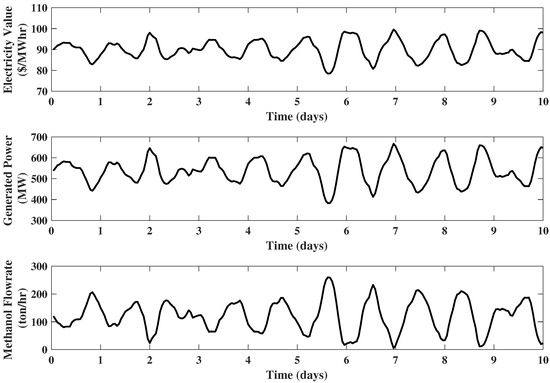
Now, set the value of to , and investigate the impact of different methanol prices (). For this case, the solution to Problem (70) is provided in Table 7. When the methanol price equals $90/ton MeOH, the solution indicates that no methanol synthesis reactor system is needed. However, in order to take advantage of the electricity price fluctuations, a hydrogen storage unit with a capacity of 355.2 tons and a new power generation unit with a capacity of 269.2 MW are required. When is increased to 100$/ton MeOH, we have the same case as in Table 6. When is increased to 200 $/ton MeOH, a larger methanol reactor synthesis system is required ( tons MeOH/h), and the generated power stays at its minimum ( MW). No hydrogen storage is needed, which indicates all the extra hydrogen flows into the methanol synthesis reactor system to generate methanol. Regarding the process simulations using the controller generated from Problem (70), the case of =$90/ton MeOH is illustrated in Figure 16.
Table 7.
Optimal design results as a function of methanol price.
Figure 16.
Value of electricity and the resulting power generation dispatch for the case of and $/ton MeOH.
Finally, let us consider the impact of equipment cost on the optimal design. Specifically, assume that the values of compressor cost coefficients are reduce to , , , . Furthermore, assume the methanol price () to be 100 $/ton MeOH. Then, the solution to Problem (70) for different values of is given in Table 8. The process simulations for the case of are illustrated in Figure 17, Figure 18 and Figure 19.
Table 8.
Optimal design results as a function of electricity price variance with reduced capital costs of compressors.
Figure 17.
Value of electricity and the resulting power generation dispatch for the case of and $/ton MeOH with reduced compressors costs.
Figure 18.
Value of electricity and the resulting air compressor power consumption dispatch for the case of and $/ton MeOH with reduced compressors costs.
Figure 19.
Value of electricity and the resulting compressor power consumption dispatch for the case of and $/ton MeOH with reduced compressors costs.
5. Conclusions
This work presented the integrated design and control of an IGCC power dispatch system using economic linear optimal control. The upgrade scenarios included compressed air storage, hydrogen storage, carbon dioxide storage, power generation block expansion, air compressor, carbon dioxide compressor, and the methanol synthesis reactor system. For the assumed set of economic parameters, it was found that hydrogen storage, power generation block expansion, and the methanol synthesis reactor system were the preferable options, whereas the compressed air storage, carbon dioxide storage, additional air compressor, and carbon dioxide compressor were not desired. However, if the capital costs of air compressor and carbon dioxide compressor were reduced, the optimal design of the IGCC power dispatch system would prefer to add these equipment and corresponding storage units when the variance of electricity price is large. The approach provided in this paper overcomes the limitation of economic MPC in the design problem through use of ELOC as a surrogate control policy.
Author Contributions
J.Z. and S.G.F. built the models, ran the simulations, post-processed, analyzed the results, and wrote the manuscript. D.J.C. contributed to supervising, reviewing of the results, and revising the manuscript. All authors read and agreed to the published version of the manuscript.
Funding
This research was funded by the National Science Foundation (CBET-1511925).
Conflicts of Interest
The authors declare no conflict of interest.
Abbreviations
The following abbreviations are used in this manuscript:
| ASU | Air Separation Unit |
| ELOC | Economic Linear Optimal Control |
| EMPC | Economic Model Predictive Control |
| IGCC | Integrated Gasification Combined Cycle |
References
- Chmielewski, D.J. Smart grid: The basics—What? Why? Who? How? Chem. Eng. Prog. 2014, 110, 28–34. [Google Scholar]
- Robinson, P.J.; Luyben, W.L. Plantwide control of a hybrid integrated gasification combined cycle/methanol plant. Ind. Eng. Chem. Res. 2011, 50, 4579–4594. [Google Scholar] [CrossRef]
- Jones, D.; Bhattacharyya, D.; Turton, R.; Zitney, S.E. Optimal design and integration of an air separation unit (ASU) for an integrated gasification combined cycle (IGCC) power plant with CO2 capture. Fuel Process. Technol. 2011, 92, 1685–1695. [Google Scholar] [CrossRef]
- Mahapatra, P.; Bequette, B.W. Process design and control studies of an elevated-pressure air separations unit for IGCC power plants. In Proceedings of the American Control Conference, Baltimore, MD, USA, 30 June–2 July 2010. [Google Scholar]
- Bequette, B.W.; Mahapatra, P. Model Predictive Control of Integrated Gasification Combined Cycle Power Plants: Technical Report; OSTI ID: 1026486; Department of Energy (DOE): Washington, DC, USA, 2010.
- Rawlings, J.B.; Angeli, D.; Bates, C.N. Fundamentals of economic model predictive control. In Proceedings of the IEEE Conference on Decision and Control (CDC), Maui, HI, USA, 10–13 December 2012. [Google Scholar]
- Rawlings, J.B. Tutorial overview of model predictive control. IEEE Control Syst. Mag. 2000, 20, 38–52. [Google Scholar]
- Henze, G.P.; Krarti, M.; Brandemuehl, M.J. Guidelines for improved performance of ice storage systems. Energy Build. 2003, 35, 111–127. [Google Scholar] [CrossRef]
- Braun, J.E. Impact of control on operating costs for cool storage systems with dynamic electric rates. ASHRAE Trans. 2007, 113, 343–354. [Google Scholar]
- Mendoza-Serrano, D.I.; Chmielewski, D.J. Infinite-horizon economic MPC for HVAC systems with active thermal energy storage. In Proceedings of the 51st IEEE Conference on Decision and Control, Maui, HI, USA, 10–13 December 2012. [Google Scholar]
- Mendoza-Serrano, D.I.; Chmielewski, D.J. Smart grid coordination in building HVAC systems: EMPC and the impact of forecasting. J. Process Control 2014, 24, 1301–1310. [Google Scholar] [CrossRef]
- Karwana, M.H.; Keblisb, M.F. Operations planning with real time pricing of a primary input. Comput. Oper. Res. 2007, 34, 848–867. [Google Scholar] [CrossRef]
- Baumrucker, B.T.; Biegler, L.T. MPEC strategies for cost optimization of pipeline operations. Comput. Chem. Eng. 2010, 34, 900–913. [Google Scholar] [CrossRef]
- Lima, R.M.; Grossmann, I.E.; Jiao, Y. Long-term scheduling of a single-unit multi-product continuous process to manufacture high performance glass. Comput. Chem. Eng. 2011, 35, 554–574. [Google Scholar] [CrossRef]
- Kostina, A.M.; Guillén-Gosálbeza, G.; Meleb, F.D.; Bagajewiczc, M.J.; Jiméneza, L. A novel rolling horizon strategy for the strategic planning of supply chains: Application to the sugar cane industry of Argentina. Comput. Chem. Eng. 2011, 35, 2540–2563. [Google Scholar] [CrossRef]
- Omell, B.P.; Chmielewski, D.J. IGCC power plant dispatch using infinite-horizon economic model predictive control. Ind. Eng. Chem. Res. 2013, 52, 3151–3164. [Google Scholar] [CrossRef]
- Omell, B.P.; Chmielewski, D.J. Application of infinite-horizon EMPC to IGCC dispatch. In Proceedings of the American Control Conference, Washington, DC, USA, 17–19 June 2013. [Google Scholar]
- Adeudo, O.; Omell, B.P.; Chmielewski, D.J. On the theory of economic MPC: ELOC and approximate infinite horizon EMPC. J. Process Control 2019, 73, 19–32. [Google Scholar] [CrossRef]
- Mendoza-Serrano, D.I.; Chmielewski, D.J. Demand response for chemical manufacturing using Economic MPC. In Proceedings of the American Control Conference, Washington, DC, USA, 17–19 June 2013. [Google Scholar]
- Feng, J.; Brown, A.; O’Brien, D.; Chmielewski, D.J. Smart grid coordination of a chemical processing plant. Chem. Eng. Sci. 2015, 136, 168–176. [Google Scholar] [CrossRef]
- Adeudo, O.; Chmielewski, D.J. Control of electric power transmission networks with massive energy storage using economic MPC. In Proceedings of the American Control Conference, Washington, DC, USA, 17–19 June 2013. [Google Scholar]
- Köhler, J.; Müller, M.A.; Li, N.; Allgöwer, F. Real time economic dispatch for power networks: A distributed economic model predictive control approach. In Proceedings of the IEEE 56th Annual Conference on Decision and Control (CDC), Melbourne, Australia, 12–15 December 2017. [Google Scholar]
- Standardi, L. Economic Model Predictive Control for Large-Scale and Distributed Energy Systems. Ph.D. Thesis, Technical University of Denmark, Kongens Lyngby, Denmark, 2015. [Google Scholar]
- Rodríguez, D.I.H.; Myrzik, J.M.A. Economic model predictive control for optimal operation of home microgrid with photovoltaic-combined heat and power storage Systems. IFAC PapersOnLine 2017, 50, 10027–10032. [Google Scholar]
- Chmielewski, D.J.; Manthanwar, A.M. On the tuning of predictive controllers: Inverse optimality and the minimum variance covariance constrained control problem. Ind. Eng. Chem. Res. 2004, 43, 7807–7814. [Google Scholar] [CrossRef]
- Peng, J.K.; Manthanwar, A.M.; Chmielewski, D.J. On the tuning of predictive controllers: The minimum back-off operating point selection problem. Ind. Eng. Chem. Res. 2005, 44, 7814–7822. [Google Scholar] [CrossRef]
- Omell, B.P.; Chmielewski, D.J. On the tuning of predictive controllers: Impact of disturbances, constraints, and feedback structure. AICHE J. 2014, 60, 3473–3489. [Google Scholar] [CrossRef]
- Zhang, J.; Omell, B.P.; Chmielewski, D.J. On the tuning of predictive controllers: Application of generalized Benders decomposition to the ELOC problem. Comput. Chem. Eng. 2015, 82, 105–114. [Google Scholar] [CrossRef]
- Mendoza-Serrano, D.I.; Chmielewski, D.J. Smart grid coordination in building HVAC systems: Computational efficiency of constrained ELOC. Sci. Technol. Built Environ. 2015, 21, 812–823. [Google Scholar] [CrossRef]
- Mendoza-Serrano, D.I.; Chmielewski, D.J. Optimal chiller and thermal energy storage design for building HVAC systems. In Proceedings of the International High Performance Buildings Conference, Purdue, IN, USA, 14–17 July 2014. [Google Scholar]
- Adeudo, O.; Chmielewski, D.J. EMPC-based design of energy storage units for electric power networks. In Proceedings of the American Control Conference, Seattle, WA, USA, 24–26 May 2017. [Google Scholar]
- Mendoza-Serrano, D.I.; Chmielewski, D.J. A two-stage procedure for the optimal sizing and placement of grid-level energy storage. Comput. Chem. Eng. 2018, 114, 265–272. [Google Scholar]
- Yang, M.W.; Omell, B.P.; Chmielewski, D.J. Controller design for dispatch of IGCC power plants. In Proceedings of the American Control Conference, Montreal, QC, Canada, 27–29 June 2012. [Google Scholar]
- Zoelle, A.; Keairns, D.; Turner, M.J.; Woods, M.; Kuehn, N.; Shah, V.; Chou, V.; Pinkerton, L.L.; Fout, T. Cost and Performance Baseline for Fossil Energy Plants Volume 1b: Bituminous Coal (IGCC) to Electricity Revision 2b—Year Dollar Update. United States. Available online: https://www.osti.gov/biblio/1480991-cost-performance-baseline-fossil-energy-plants-volume-bituminous-coal-igcc-electricity-revision-year-dollar-update (accessed on 29 January 2020). [CrossRef]
- Anderson, B.D.O.; Moore, J.B. Optimal Filtering; Prentice Hall: Englewood Cliffs, NJ, USA, 1979. [Google Scholar]
- Bagajewicz, M.J.; Manousiouthakis, V. On the generalized benders decomposition. Comput. Chem. Eng. 1991, 15, 691–700. [Google Scholar] [CrossRef]
- Geoffrion, A.M. Generalized benders decomposition. J. Optim. Theory Appl. 1972, 10, 237–260. [Google Scholar] [CrossRef]
- Luenberger, D.G. Investment Science; Oxford University Press: New York, NY, USA, 1998. [Google Scholar]


© 2020 by the authors. Licensee MDPI, Basel, Switzerland. This article is an open access article distributed under the terms and conditions of the Creative Commons Attribution (CC BY) license (http://creativecommons.org/licenses/by/4.0/).