An Online Contaminant Classification Method Based on MF-DCCA Using Conventional Water Quality Indicators ^†

Abstract

Emergent contamination warning systems are critical to ensure drinking water supply security. After detecting the existence of contaminants, identifying the types of contaminants is conducive to taking remediation measures. An online classification method for contaminants, which explored abnormal fluctuation information and the correlation between 12 water quality indicators adequately, is proposed to realize comprehensive and accurate discrimination of contaminants. Firstly, the paper utilized multi-fractal detrended fluctuation analysis (MF-DFA) to select indicators with abnormal fluctuation, used multi-fractal detrended cross-correlation analysis (MF-DCCA) to measure the cross-correlation between indicators. Subsequently, the algorithm fused the abnormal probability of each indicator and constructed the abnormal probability matrix to further judge the abnormal fluctuation of indicators using D–S evidence theory. Finally, the singularity index of the cross-correlation function and the selected indicators were used to classification by cosine distance. Experiments of five chemical contaminants at three concentration levels were implemented, and analysis results show the method can weaken disturbance of water quality background noise and other interfering factors. It effectively improved the classification accuracy at low concentrations compared with another three methods, including methods using triple standard deviation threshold and single indicator fluctuation analysis-only methods without fluctuation analysis. This can be applied to water quality emergency monitoring systems to reduce contaminant misclassification.

1. Introduction

The frequent occurrence of emergent contamination events in drinking water pipes poses a great threat to drinking water supply security. It is particularly critical to establish a sound emergency warning system for water environmental pollution [1,2]. The accurate and timely classification of contaminants is conducive to taking targeted measures to deal with pollution sources, which is an important prerequisite for water rescue work.

Contaminant classification methods used most commonly is the laboratory-based analysis, e.g., ICP-MS. It has the advantages of low detection limit and high precision, and support contaminants classification and quantitative analysis. However, this method is time-consuming and difficult to meet the needs for online classification in the water quality warning system. Some researchers use online compound-specific sensors to detect the type of contaminants. Although this method faster than the laboratory-based analysis, it can normally only identify one type or a small group of contaminants [3,4,5]. Some scholars have tried to develop online methods for identifying contaminants using conventional water quality indicators considering that using conventional indicators to analyze water quality is suitable for online monitoring with fast analysis speed. Online classification of contaminants in water pipelines is mainly based on supervised classification methods at present. Kroll et al. [6] processed five independent water quality parameters (pH, Conductivity, Turbidity, Residual Chlorine, and TOC) into a single trigger signal, and the direction of the deviation signal was related to the nature of contaminants. Based on the experimental data, the deviation signal library was established, and the contaminants could be distinguished by comparing the deviation signal with the signal in the library. Yang et al. [7] studied the changes of different water quality indicators caused by 11 kinds of contaminants based on the real-time adaptive signal processing method, established four contaminants classification systems, and used the geometric characteristics of the response of water quality indicators to distinguish the categories of contaminants. Liu et al. [8] used the clustering algorithm to get the class center of the contaminant response signal, and measured the similarity between the monitored sample value and the class center by calculating the Mahalanobis distance to identify the contaminants. The team [9] then employed cosine distances to measure similarities to determine the category of contaminants. Compared with the Mahalanobis distance, it can better reduce the influence caused by unknown concentrations of contaminants. Huang et al. [10] proposed a multi-classification model based on support vector machine (SVM) for contaminant classification, and introduced the classification probability to distinguish contaminants. To some extent, it avoided making a single decision when classification features were unclear in the initial phase of contaminants injection.

There are problems of information redundancy and low signal-to-noise ratio in conventional water quality indicators data, affected by the sensors and fluctuation of water quality background. It is difficult to identify the contaminants when the concentration of contaminants is low in the early stage of sudden pollution incidents. The existing methods for online classification of contaminants based on conventional water quality indicators have achieved relatively good classification results. However, multiple water quality indicators show linkage changes during the occurrence of sudden water pollution incidents, and the above methods do not fully explore the correlation and difference among indicators with abnormal fluctuations caused by contaminants, which limits the accuracy of contaminant classification to some extent at low concentrations.

Considering the above problem of the online classification of contaminants, this paper proposes an online classification method for contaminants in water pipelines based on cross-correlation analysis combined with D–S evidential theory. Firstly, the paper picked out the indicators series with abnormal fluctuation utilizing multi-fractal detrended fluctuation analysis (MF-DFA) and measured the cross-correlation between these selected water quality indicators series based on multi-fractal detrended cross-correlation analysis (MF-DCCA). Then, the paper fused the abnormal probability of each indicator and constructed the abnormal probability matrix to further judge the abnormal fluctuation of indicators using D–S evidence theory. Finally, the singularity index of the cross-correlation function and the time series of the selected indicators formed eigenvectors and implemented contaminant classification using cosine distance. Compared with another three methods, the proposed approach effectively filtered out signal noise and other interfering factors by further exploring the cross-correlation between indicators. It revealed the hydrodynamic characteristics of different contaminants hidden in complex data and improved the classification accuracy at low concentrations.

2. Methods and Experiment

2.1. Principles and Methodology

The online contaminant classification method proposed in this paper is mainly based on MF-DCCA (multi-fractal detrended cross-correlation analysis) and D–S evidential theory.

The workflow of the method is shown in Figure 1, which is specifically divided into four parts: abnormal fluctuation analysis of single indicator, cross-correlation analysis of multiple indicators with abnormal fluctuation, abnormal probability information fusion, and classification based on cosine distance. This paper used the MF-DFA algorithm to evaluate the fluctuation of the time series of all the indicators firstly, secondly analyzed the cross-correlation of indicators screened in the previous step based on MF-DCCA algorithm, and then the judgment results from different sensors monitoring water quality indicators were used to complete the information fusion at the decision-making level utilizing D–S evidential theory. Finally, the fused information was used as auxiliary evidence combined with the selected anomalous fluctuation indicators series to form feature vectors for identification.

2.1.1. Abnormal Fluctuation Analysis of Single Indicator Based on MF-DFA

The multifractal detrended fluctuation analysis (MF-DFA) was proposed by Kantelhardt with the aim to detect multifractal properties of nonlinear and nonstationary time series, which provides efficient tools for estimation of the multifractal spectrum. The technical details of MF-DFA are mentioned in [11]. In this paper, MF-DFA was used to analyze the time series of conventional water quality indicators. For a nonstationary time series of indicators with a length of $N$, $x_k\left(i=1, 2,\dots , N\right)$, the multifractal spectrum $f\left(\alpha \right)$ can be obtained after analysis.

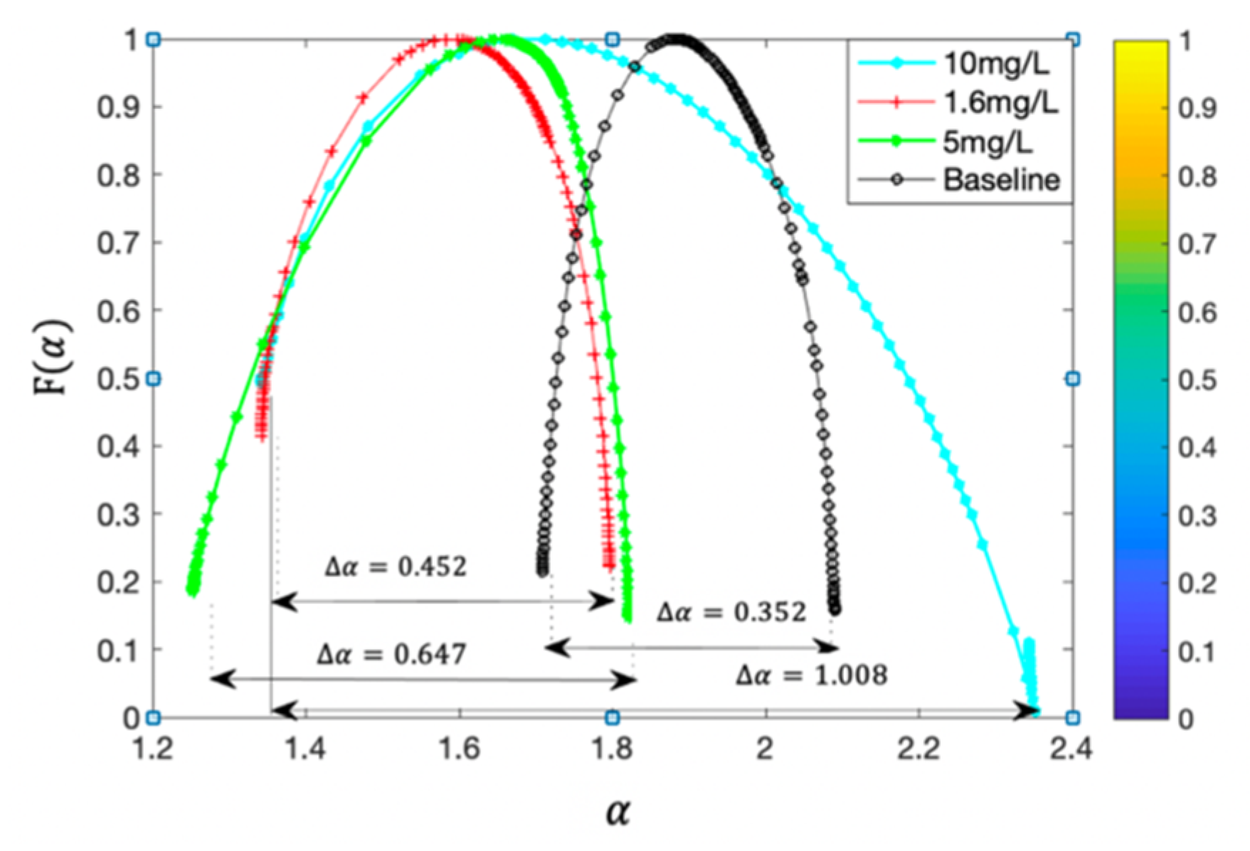
As shown in Figure 2, it is the analysis result for Ammonia Nitrogen time series data for the injection of Copper Sulfate with different concentrations.$f\left(\alpha \right)$ is a smooth convex curve with a single peak, and its x-coordinate$\alpha$ is a singular index, reflecting the growth probability of the fractal in a small region. $\Delta \alpha =\alpha \left(-\infty \right)- \alpha \left(+\infty \right)$ indicates the inhomogeneity of the distribution of the Ammonia Nitrogen time series in the whole probability measure. The larger the $\Delta \alpha$, the stronger the multifractal properties.

The $\Delta \alpha$ of each indicator time series was compared with the corresponding threshold, and the $\alpha \left(0\right)$ was used as auxiliary information to judge whether the indicator had abnormal fluctuation or not. The specific fluctuations of these indicators caused by current contaminants were measured, the water quality indicators without abnormal fluctuation or unapparent abnormal fluctuation (equivalent to noise signal) were eliminated, and then the time series of indicators with real abnormal fluctuation were used for the next processing, which can effectively weaken the disturbance of water background fluctuation and other noise.

2.1.2. Cross-correlation Analysis of Multiple Indicators Based on MF-DCCA

Multifractal detrended cross-correlation analysis (MF-DCCA) was proposed by Zhou [12] to reveal the multifractal features of two nonstationary time series, and it finds applications ranging from investment market [13,14,15], environmental analysis [16,17,18], biomedical [19,20,21], traffic data [22], and power industry [23]. The technical details of MF-DCCA is mentioned in [12].

$x\left(i\right)$ and $y\left(i\right)$ are time series data of water quality indicators, $i=1,2,\dots N$, and the analysis process of these two water quality indicators using MF-DCCA is as follows:

• Divide $x\left(i\right)$ and $y\left(i\right)$ into $N_s$ pieces of data of length s, that is, $N_s=\frac{N}{s}$.
• Calculate the cross-correlation fluctuation function between $x\left(i\right)$ and $y\left(i\right)$:

  $$F_s\left(s\right)=\frac{1}{s}{\displaystyle \sum }_{k=1}^s[X_v\left(k\right)-\widetilde{X_v}\left(k\right)][Y_v\left(k\right)-\widetilde{Y_v}\left(k\right)]$$

  (1)

  $$X_v\left(k\right)={{\displaystyle \sum }}_{j=1}^{k}x[\left(v-1\right)s+j]$$

  (2)

  $$Y_v\left(k\right)={{\displaystyle \sum }}_{j=1}^{k}y[\left(v-1\right)s+j],v=1,2,\dots N_s, k=1,2,\dots s$$

  (3)

  $\widetilde{X_v}\left(k\right)$ and $\widetilde{Y_v}\left(k\right)$, respectively, represent the local trend of time series $X_v\left(k\right)$ and $Y_v\left(k\right)$.
• Calculate the de-trending covariance function of order q between time series $x\left(i\right)$and $y\left(i\right)$:

  $$\{\begin{array}{c}{F}_{xy}\left(q,s\right)={\left[\frac{1}{N}{\displaystyle {\displaystyle \sum }_{v=1}^{N_s}}{F}_v{\left(s\right)}^{\frac{2}{q}}\right]}^{\frac{1}{q}}q\ne 0\\ F_{xy}\left(0,s\right)=exp{\left[\frac{1}{2N}{\displaystyle {\displaystyle \sum }_{v=1}^{N_s}}ln{F}_v\left(s\right)\right]}^{\frac{1}{q}}q=0\end{array}$$

  (4)

(1)

When there is a long-range correlation between time series $x\left(i\right)$and $y\left(i\right)$, the relationship between $F_q\left(s\right)$ and $s$ is as follows:

$$F_{xy}\left(q,s\right) ~ {\mathrm{s}}^{h_{xy}\left(q\right)}$$

(5)

$h_{xy}\left(q\right)$ is a generalized cross-correlation Hurst exponent.

(2)

The de-trend cross-correlation index of time series $x\left(i\right)$and $y\left(i\right)$ is:

$${\tau }_{xy}\left(q\right)=q{h}_{xy}\left(q\right)-1$$

(6)

According to the Legendre transformation, we can get this relationship:

$$\alpha =\frac{d{\tau }_{xy}\left(q\right)}{d\left(q\right)}=h_{xy}\left(q\right)+q{h^{\prime }}_{xy}\left(q\right)$$

(7)

$$f_{xy}\left(\alpha \right)=q\alpha -{\tau }_{xy}\left(q\right)=q[\alpha -h_{xy}\left(q\right)]+1$$

(8)

In this paper, according to the water quality indicators series with abnormal fluctuation screened out in the previous step, the MF-DCCA algorithm was employed to analyze the multifractal features of the cross-correlation functions of each two indicators series. MF-DCCA (multi-fractal detrended cross-correlation analysis) fully considers the cross-correlation between data. So, it can better exclude the influence of signal noise and other factors on the results, and explore the dynamic mechanism hidden in the data effectively. Based on the multifractal spectrum, five eigenvalues with explicit physical meaning can be extracted to form an eigenvector:

$$[\alpha \left(+\infty \right) f\left(\alpha \left(+\infty \right) \right) \alpha \left(0\right) \alpha \left(-\infty \right) f\left(\alpha \left(-\infty \right) \right)],$$

which enables a more complete description of the fluctuations of nonstationary time series. The width of the spectrum $\Delta \alpha$, equivalent to $\alpha \left(-\infty \right)- \alpha \left(+\infty \right)$, describes the strength of multifractality. The larger the ∆α, the stronger the cross-correlation between the indicators.

If $\Delta {\alpha }_{xy}$ based on the time series$x\left(t\right)$ and$y\left(t\right)$ is equal to the threshold $C$, it indicates that the time series of the two water quality indicators are at the critical point of relevant and irrelevant. When $\Delta {\alpha }_{xy}>C$, it indicates that there is a strong correlation. When $\Delta {\alpha }_{xy}<C$, it shows that there is no correlation or weak correlation between them.

2.1.3. Abnormal Probability Fusion Based on D–S Evidential Theory

D–S evidential theory was first proposed by professor Dempster [24] of Harvard University in 1967 and further improved by his student Shafer [25] in 1976, which plays an important role in multi-source information fusion in the fields of target recognition, water environment monitoring, and medical diagnosis [26,27,28,29,30,31]. In this paper, D–S evidential theory was used to fuse and analyze the abnormal fluctuation of multiple water quality indicators. The recognition frame$\Theta$ consists of two elements: Normal and Abnormal.

Define the basic probability distribution function as follows:

$$\{\begin{array}{c}m\left(Normal\right)=\frac{1}{1+e^{-\left(\Delta {\partial }_j\left(t\right)\right)}}\\ m\left(Abnormal\right)=1-m\left(Normal\right)\end{array}$$

(9)

$\Delta {\partial }_j=\Delta {\alpha }_j-A$ represents the degree to which the scale index $\Delta {\alpha }_j$ deviates from the threshold $A$. $\Delta {\alpha }_j$ is the degree of unevenness of the$j$-th indicator time series based on MF-DFA.

Multi-indicators anomaly probability fusion adopts the form of confidence accumulation:

$$P\left(Normal\right)={\displaystyle \prod }_{i=1}^{n}m\left(Normal,X_i\right)$$

(10)

where the basic abnormal probability of indicator $i$ is denoted as$m\left(Abnormal,x_i\right)=p_i$, and the cross-correlation index $\Delta {\alpha }_{xy}$ of water quality indicator $i, j$ is normalized to $d_{ij}$. So, the abnormal probability of cross-correlation of each two indicators among N water quality indicators is as follows:

$$P\left(X_i\left(t\right),X_j\left(t\right)\right)=\left\{1-\left(1-p_i\right)·\left(1-d_{ij}\right)·\left(1-p_j\right)\right\} i,j,\dots ,N$$

(11)

2.1.4. Constructing Eigenvector and Classifying Based on Cosine Distance

The abnormal probability matrix is obtained from Equation (11), and used the threshold to judge whether the fusion probability of the two associated indicators is abnormal. If the judgment result is abnormal, the normalized cross-correlation index $d_{ij}$ and the time series of the corresponding indicators are combined to form a feature vector, and the relevant data is needed to be taken out from the contaminant information library. If it is judged to be normal, it indicates that at least one of the two indicators are not of abnormal fluctuation, and there is no need to extract relevant information from the information library. When the eigenvector is constructed, online classification can be carried out based on cosine distance.

Cosine distance is a measure of similarity based on the cosine of the angle between two vectors [32,33]:

$$Similaity\left(p,q\right)=cos\theta =\frac{pq}{\left|\right|p\left|\right|\left|\right|q\left|\right|}=\frac{{{\displaystyle \sum }}_{i=1}^n{p}_i\times q_i}{\sqrt{{{\displaystyle \sum }}_{i=1}^n{\left(p_i\right)}^2}\times \sqrt{{{\displaystyle \sum }}_{i=1}^n{\left(q_i\right)}^2}}$$

(12)

where the smaller the angle$\theta$ between vector $p\mathrm{and} \mathrm{vector}q$ is, the closer the cosine distance $cos\theta$ is to 1, that is, the more similar the two vectors are.

Compared with the measurement method based on Euclidean Distance, the cosine distance excludes the influence of the vector′s amplitude. When the same contaminant is injected to the water pipeline with different concentrations, the amplitude of the abnormal fluctuation of the indicators is different. So, using the cosine distance for classification can weaken the influence of different concentrations.

2.2. Part of the Experiment

2.2.1. Experimental Apparatus

All experiments involved in this paper were conducted in the simulated water pipeline system. The structure of the system is shown in Figure 3, consisting of three parts: automatic chemicals feeding system, chemicals mixing system, and automatic monitoring system. In Figure 3a, the numbers (1)–(11) represent, respectively: (1) water from pipeline; (2) dosing bucket; (3) water tank; (4) recycling bin; (5) flowmeter; (6) toxic instrument; (7) total phosphorus and Total Nitrogen analyzer; (8) Potassium permanganate index analyzer; (9) Turbidity meter; (10) Residual Chlorine analyzer; and (11) conventional five-parameter analyzer. There are twelve conventional water quality indicators used in this paper, including pH, Conductivity, Turbidity, Dissolved Oxygen, COD, Permanganate Indicator, TOC, Ammonia Nitrogen, Nitrate Nitrogen, Total Phosphorus, Total Nitrogen, and Residual Chlorine.

2.2.2. Experimental Scheme Design

The experiment was divided into two phases. The first phase was to build a contaminants library of water quality indicators response, the second phase was to verify the performance of the algorithm using the data obtained from the new contaminants’ injection experiments. In this experiment, three classes and five types of the most common contaminants were selected, including agricultural contaminants (Ammonium Citrate), chemical contaminants (Potassium Hydrogen Phthalate, Sodium Nitrite, Potassium Ferricyanide), and heavy metal contaminants (Copper Sulfate). The five types of contaminants were employed to construct the contaminants library, and Copper Sulfate was taken as an example to demonstrate the performance of the classification algorithm in the paper.

1. Build Contaminants Library

In the first phase, the dilution ratio of the water pipeline system was adjusted to 2%, and five concentration gradients were set for each contaminant to conduct an experiment with the injection interval of 30 min. The concentrations of the sample solution were 400, 300, 200, 100, and 50 mg/L, and the concentrations of contaminants actually presented in the main pipeline after dilution were 8, 6, 4, 2, and 1 mg/L. The information of contaminants concentration and number of sampling points is shown in

Table 1. Information on characteristic contaminants used for training.

Chemicals	Concentration of Chemicals	Concentration of Contaminants	Number of Sampling Point
Ammonium Citrate	400 mg/L	8 mg/L	30
Potassium Hydrogen Phthalate	300 mg/L	6 mg/L	30
Sodium Nitrite	200 mg/L	4 mg/L	30
Potassium Ferricyanide	100 mg/L	2 mg/L	30
Copper Sulfate	50 mg/L	1 mg/L	30

. The sampling interval was set to 1 min. The time series of all water quality indicators were obtained from the sensors, and characteristics information of contaminants was added into the knowledge library after analysis using the proposed algorithm.

2. Obtain Contaminant Classification Data

In the second phase of the experiment, the five kinds of contaminants mentioned above were used for new injection experiments to demonstrate the performance of algorithm. The concentrations of the sample solution were 500, 250, and 80 mg/L, and the concentrations of contaminants actually presented in the main pipeline after dilution were 10, 5.0, and 1.6 mg/L. The information of contaminants concentration and sampling points is shown in

Table 2. Information on characteristic contaminants used for testing.

Chemicals	Concentration of Chemicals	Concentration of Contaminants	Number of Sampling Point
	500 mg/L	10 mg/L	30
Five kinds of contaminants	250 mg/L	5.0 mg/L	30
	80 mg/L	1.6 mg/L	30

. The data collected by the sensors after the abnormal detection was used for online classification of characteristic contaminants. There were 30 samples in each group of contaminants.

3. Results and Discussion

3.1. The Result of Single Indicator Fluctuation Analysis

The MF-DFA algorithm was used to evaluate the fluctuation of the time series of twelve indicators, and the Hurst graph and the multifractal singular spectrum were obtained. Taking the concentration of 10 mg/L as an example, the Hurst graph and the multifractal singular spectrum of Nitrate Nitrogen are shown in Figure 4, the value $\Delta {\alpha }_j$ extracted from the spectrum of all indicators are shown in

Table 3. The results of single indicator fluctuation analysis.

	Contaminants	(1)	(2)	(3)	(4)	(5)	(6)
Indicators
pH		0.239	0.457	0.529	0.244	0.721	0.218
Conductivity		0.314	0.349	0.297	0.295	0.326	0.307
Turbidity		0.198	0.323	0.176	0.185	0.443	0.632
Dissolved Oxygen		0.562	0.690	0.723	0.476	0.396	0.891
COD		0.881	1.038	0.989	1.149	1.324	0.923
Permanganate Indicator		0.135	0.118	0.126	0.148	0.154	0.147
TOC		0.947	1.125	2.846	1.221	1.336	0.996
Ammonia Nitrogen		0.352	1.469	0.456	1.983	1.009	0.380
Nitrate Nitrogen		0.702	0.626	1.271	0.746	0.665	0.896
Total Phosphorus		0.149	0.155	0.137	0.142	0.162	0.128
Total Nitrogen		0.165	0.169	0.154	0.138	0.161	0.157
Residual Chlorine		0.427	0.477	0.394	0.975	1.437	0.451

(1)–(6) represent no contaminants added, Ammonium Citrate, Potassium Hydrogen Phthalate, Potassium Ferricyanide, Copper Sulfate, Sodium Nitrite.

.

Under normal circumstances, the background fluctuation intensity of different water quality indicators was different, and the more severe the fluctuation was, the higher the value $\Delta {\alpha }_j$ was. For example, the background fluctuation of the time series of COD, TOC, Nitrate Nitrogen was more obvious than Turbidity, Permanganate Indicator, Total Phosphorus, and Total Nitrogen. Taking Residual Chlorine as an example, the injection of Potassium Ferricyanide and Copper Sulfate caused obvious fluctuation in Residual Chlorine’s time series, and other contaminants had little effect on it. Substituting the difference between $\Delta {\alpha }_j$and the preset threshold into the basic probability distribution function better described the abnormal fluctuations of a single indicator, and the water quality indicators without abnormal fluctuations (corresponding to noise signals) were eliminated.

3.2. Cross-Correlation Analysis of Multiple Indicators and Comparison of Probability Fusion Results

MF-DCCA and D–S evidential theory were used to analyze the multifractal features of each two indicators time series and obtain the abnormal probability matrix. Figure 5a,b, respectively, show the abnormal probability results of water quality indicators before and after the introduction of multi-indicators correlation information. The numbers 1 to 12 represent 12 water quality indicators, namely pH, Conductivity, Turbidity, Dissolved Oxygen, COD, Permanganate Indicator, TOC, Ammonia Nitrogen, Nitrate Nitrogen, Total Phosphorus, Total Nitrogen, and Residual Chlorine. The letters A to F represent five characteristic contaminants, namely Ammonium Citrate, Potassium Hydrogen Phthalate, Potassium Ferricyanide, Copper Sulfate, and Sodium Nitrite. The abnormal fluctuation probability of indicators is divided into 10 grades from 0 to 1, and the corresponding color blocks are from white to black. The more obvious abnormal fluctuation is, the darker the color is.

Taking Ammonium Citrate as an example, the response curves of each indicator are shown in Figure 5 at the concentration of 1 mg/L, 2 mg/L, 4 mg/L, 6 mg/L, and 8 mg/L.

There appeared obvious fluctuations in the time series of Ammonia Nitrogen after the injection of Ammonium Citrate. In addition, pH was affected to some extent, and the fluctuation curves of other indicators did not change significantly. As shown in Figure 5a, before the introduction of MF-DCCA to analyze the cross-correlation information between the indicators, the indicators with abnormal fluctuation probability exceeding 0.7 in descending order were Ammonia Nitrogen, pH, Conductivity, TOC, and Turbidity, which was inconsistent with the results in Figure 6. During the whole experiment, the baseline of Conductivity, TOC, and Turbidity fluctuated obviously due to noise interference. If we use these three indicators time series for identification, more interference will be introduced, which will weaken the classification accuracy. As shown in Figure 5b, the indicators with abnormal fluctuation probability exceeding 0.7 in descending order only included pH and Ammonia Nitrogen when MF-DCCA was introduced to the analysis process. This is because the fluctuation correlation of other indicators was low, and the abnormal probability after fusion did not exceed the alarm threshold.

Therefore, the cross-correlation analysis for multi-indicators based on MF-DCCA can reduce the interference caused by the noise, weaken the influence of Electrical Conductivity, TOC, Turbidity, and other indicators on the results due to baseline changes and noise interference. It is helpful to improve the accuracy of contaminant classification at low concentrations.

3.3. Comparison of Contaminant Classification Results

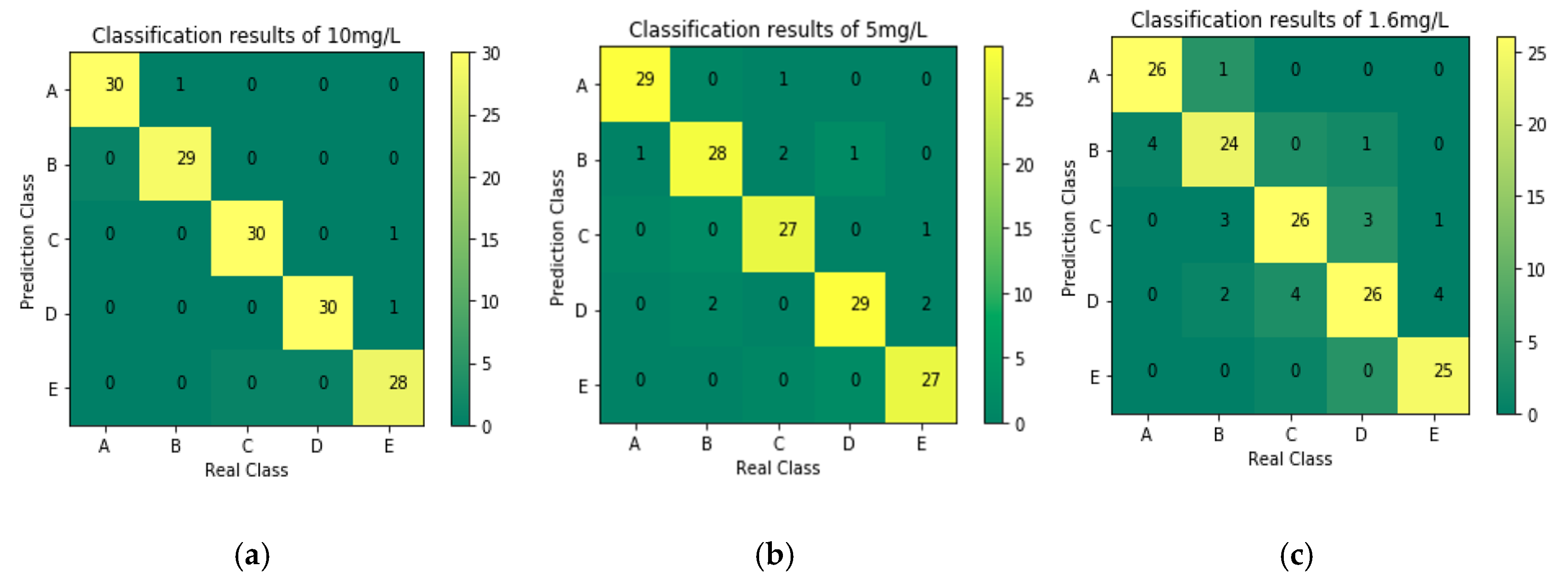
In the experiment, five types of contaminants of 10 mg/L, 5 mg/L and 1.6 mg/L were selected to verify the classification accuracy, including Ammonium Citrate, Potassium Hydrogen Phthalate, Potassium Ferricyanide, Copper Sulfate, and Sodium Nitrite. There were 30 samples for each concentration group and 90 samples for each contaminant. The normalized cross-correlation scale index and the indicator time series with abnormal fluctuations formed the feature vector, and the algorithm based on cosine distance was used to complete the contaminant classification. The recognition results are shown in Figure 7, where A, B, C, D, and E represent Ammonium Citrate, Potassium Hydrogen Phthalate, Potassium Ferricyanide, Copper Sulfate, and Sodium Nitrite. It can be seen from Figure 6 that the algorithm proposed in this paper showed good performance in identifying contaminants.

Meanwhile, in order to further verify the performance of this algorithm, the recognition accuracy before and after the introduction of cross-correlation information analysis based on MF-DCCA is presented in

Table 4. Comparison of online classification accuracy of contaminants before and after the fusion of cross-correlation information based on multi-fractal detrended cross-correlation analysis (MF-DCCA).

	Concentration(mg/L)	1.6		5		10		Average Improvement
Contaminants		Before After		Before After		Before After
Ammonium Citrate		0.73	0.87	0.93	0.97	0.97	1	7.98%
Potassium Hydrogen Phthalate		0.67	0.80	0.87	0.93	0.93	0.97	9.31%
Potassium Ferricyanide		0.70	0.87	0.83	0.90	0.97	1	10.80%
Copper Sulfate		0.77	0.90	0.90	0.97	1	1	7.49%
Sodium Nitrite		0.67	0.83	0.83	0.90	0.90	0.93	10.83%

. It can be seen that the classification accuracy of the five contaminants was significantly improved after the introduction of cross-correlation information between indicators.

Taking Copper Sulfate as an example to further illustrate the method proposed in this paper can improve the classification accuracy of contaminants at low concentrations. The classification results of Copper Sulfate are shown in Figure 8, Figure 9 and Figure 10. As the concentration decreased from 10 mg/L to 5 mg/L and 1.6 mg/L, the classification accuracy became worse, which can also be seen from Table 4. However, by comparing both parts with each other in Figure 8a,b, Figure 9a,b, and Figure 10a,b, it shows that the classification accuracy was significantly improved after the fusion of the cross-correlation information, especially for the low concentrations.

When the concentration of Copper Sulfate was 10 mg/L, as shown in Figure 8a,b, the classification accuracy was both relatively high before and after the introduction of cross-correlation information between indicators. Because for high concentrations, the signal-to-noise ratio of the time series information was high, the abnormal fluctuation was severe and the features used for recognition were obvious, therefore it had little influence on the classification results.

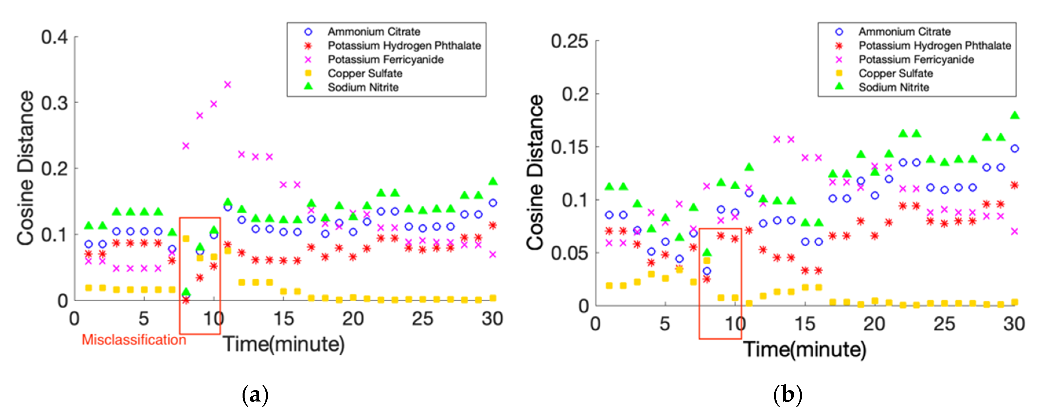
When the concentration was 5 mg/L, the classification results without the introduction of cross-correlation information are shown in Figure 9a. At the time points 8, 9, and 10, there occurred misclassification. This is because noise interference and the injection of contaminants caused different water quality fluctuations, and the indicators time series affected by noise interference had no strong correlation with other indicators series. The classification result with the introduction of cross-correlation information between indicators is shown in Figure 9b. At the time points 9 and 10, misclassification was eliminated, because the abnormal probability of the water quality indicators affected by noise such as Conductivity and TOC was lower than the alarm threshold.

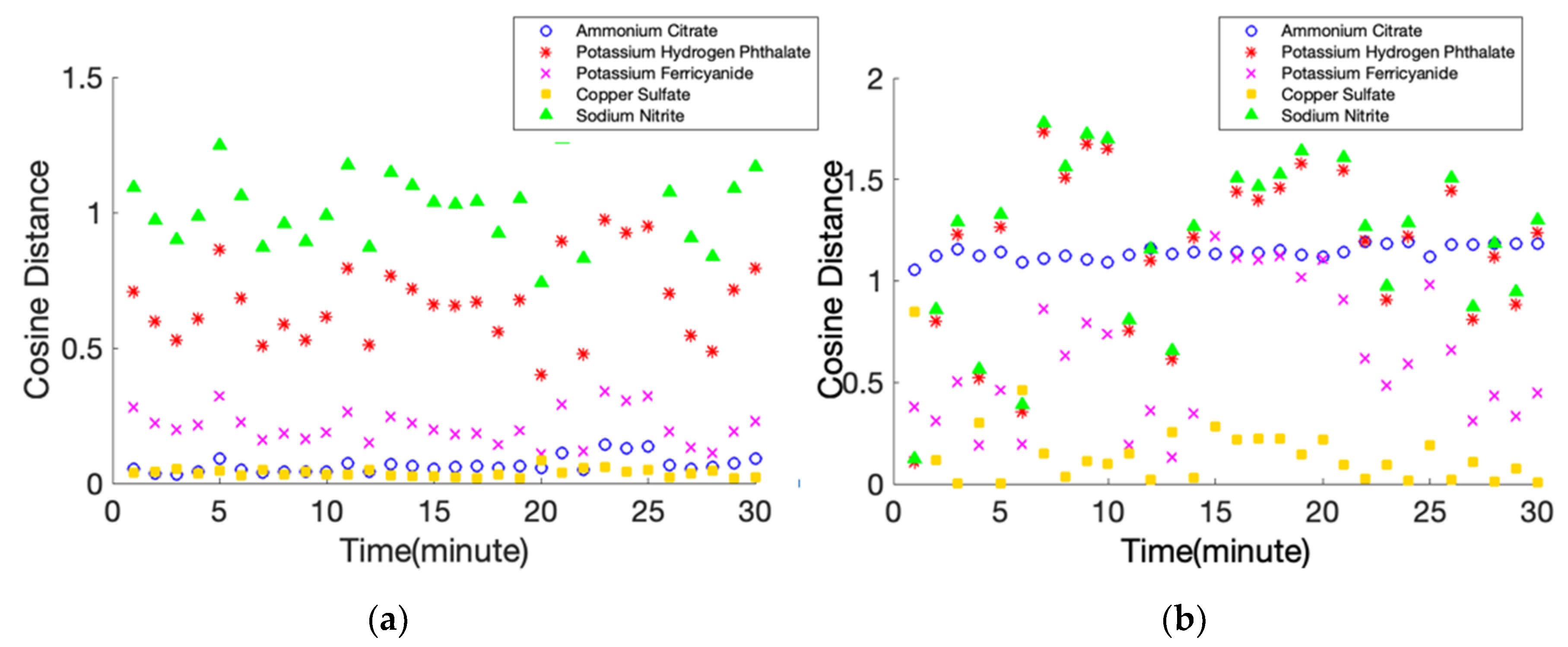
When the concentration is 1.6 mg/L, the classification results are shown in Figure 10a,b. At this time, the classification accuracy of contaminants became worse compared with the high concentration group, because as the concentration decreased, the signal-to-noise ratio was too low and the indicators data with abnormal fluctuations was hardly effectively distinguished from noise and other interference signals. However, it can be seen that the classification accuracy of Copper Sulfate increased from 0.77 before the fusion of cross-correlation information to 0.90 after fusion, which was improved by 16.89%. It demonstrates that the cross-correlation information between the indicators can effectively describe the current abnormal fluctuations, and better assist the classification work especially when the contaminants are at low concentrations.

In order to further verify the effectiveness of the proposed algorithm, this paper used three other methods to making comparisons, including the method of using all the pre-processed indicators series data for cosine distance classification directly without fluctuation analysis, the approach based on the triple standard deviation threshold, and the method only employing single indicator fluctuation analysis. The recognition results of the four methods are shown in

Table 5. Recognition results of the four methods.

	Concentration(mg/L)	1.6	5	10	Average
Methods
Method 1		0.57	0.80	0.93	0.77
Method 2		0.73	0.83	0.93	0.83
Method 3		0.77	0.90	0.99	0.87
Our method		0.90	0.98	1.00	0.96

Method 1–3 represent Method without fluctuation analysis, Method based on triple standard deviation threshold, Method based on single indicator fluctuation analysis only.

, and it is proved that the proposed algorithm effectively filtered out signal noise and other interfering factors, and it better revealed the hydrodynamic characteristics of different contaminants hidden in complex data and improve the accuracy of classification at low concentrations.

4. Conclusions

According to the characteristic that multiple conventional water quality indicators show linkage changes during the outbreak of sudden water pollution incident, this paper proposes an online classification method for contaminants in water pipeline with high precision based on multi-indicators cross-correlation analysis combined with D–S evidential theory. It is aimed to improve the classification accuracy at low concentrations in the initial stage of the sudden pollution incident by further excavating abnormal fluctuation information and the cross-correlation between water quality indicators. The paper used the method of MF-DFA to pick out the indicators series with abnormal fluctuation, utilized MF-DCCA to measure the cross-correlation between these selected water quality indicators series. Then, the method fused the abnormal probability of each indicator and constructed the abnormal probability matrix to further judge the abnormal fluctuation of indicators using D–S evidence theory. Finally, the singularity index of the cross-correlation function and the time series of the selected indicators were constructed to the eigenvectors and implemented contaminant classification by means of cosine distance.

A large number of experimental data were obtained through the injection experiment of five kinds of contaminants, and multiple sets of comparative experiments were carried out to verify the performance of the proposed algorithm, including comparing the classification results before and after the introduction of cross-correlation information, and comparing our approach with the other three methods. The results show that the proposed method can better filter out signal noise and other interfering factors, weakening the influence of abnormal fluctuation of water quality indicators caused by non-contaminants. The method effectively reveals the hydrodynamic characteristics of different contaminants hidden in complex data and improve the accuracy of classification at low concentrations.

References

1. Gullick, R.W.; Gaffney, L.J.; Crockett, C.S.; Schulte, J.; Gavin, A.J. Developing regional early warning systems for US source waters. J. Am. Water Work. Assoc. 2004, 96, 68–82. [Google Scholar] [CrossRef]
2. Storey, M.V.; Van der Gaag, B.; Burns, B.P. Advances in on-line drinking water quality monitoring and early warning systems. Water Res. 2011, 45, 741–747. [Google Scholar] [CrossRef]
3. De Hoogh, C.J.; Wagenvoort, A.J.; Jonker, F.; van Leerdam, J.A.; Hogenboom, A.C. HPLC-DAD and Q-TOF MS techniques identify cause of Daphnia biomonitor alarms in the River Meuse. Environ. Sci. Technol. 2006, 40, 2678–2685. [Google Scholar] [CrossRef]
4. Jeon, J.; Kim, J.H.; Lee, B.C.; Kim, S.D. Development of a new biomonitoring method to detect the abnormal activity of Daphnia magna using automated Grid Counter device. Sci. Total Environ. 2008, 389, 545–556. [Google Scholar] [CrossRef] [PubMed]
5. Henderson, R.K.; Baker, A.; Murphy, K.; Hambly, A.; Stuetz, R.; Khan, S. Fluorescence as a potential monitoring tool for recycled water systems: A review. Water Res. 2009, 43, 863–881. [Google Scholar] [CrossRef]
6. Kroll, D.J. Securing Our Water Supply: Protecting a Vulnerable Resource; PennWell Corporation: Tulsa, OK, USA, 2006. [Google Scholar]
7. Yang, Y.J.; Haught, R.C.; Goodrich, J.A. Real-time contaminant detection and classification in a drinking water pipe using conventional water quality sensors: Techniques and experimental results. J. Environ. Manag. 2009, 90, 2494–2506. [Google Scholar] [CrossRef] [PubMed]
8. Liu, S.M.; Che, H.; Smith, K.; Chang, T. A real time method of contaminant classification using conventional water quality sensors. J. Environ. Manag. 2015, 154, 13–21. [Google Scholar] [CrossRef] [PubMed]
9. Liu, S.M.; Che, H.; Smith, K.; Chang, T. Contaminant classification using cosine distances based on multiple conventional sensors. Environ. Sci.-Proc. Imp. 2015, 17, 343–350. [Google Scholar] [CrossRef] [PubMed]
10. Huang, P.J.; Jin, Y.; Hou, D.B.; Yu, J.; Tu, D.Z.; Cao, Y.T.; Zhang, G.X. Online Classification of Contaminants Based on Multi-Classification Support Vector Machine Using Conventional Water Quality Sensors. Sensors 2017, 17, 581. [Google Scholar] [CrossRef] [Green Version]
11. Kantelhardt, J.W.; Zschiegner, S.A.; Koscielny-Bunde, E.; Havlin, S.; Bunde, A.; Stanley, H.E. Multifractal detrended fluctuation analysis of nonstationary time series. Physica A 2002, 316, 87–114. [Google Scholar] [CrossRef] [Green Version]
12. Zhou, W.X. Multifractal detrended cross-correlation analysis for two nonstationary signals. Phys. Rev. E 2008, 77. [Google Scholar] [CrossRef] [PubMed] [Green Version]
13. Dutta, S.; Ghosh, D.; Chatterjee, S. Multifractal detrended cross correlation analysis of foreign exchange and SENSEX fluctuation in Indian perspective. Phys. A: Stat. Mech. Appl. 2016, 463, 188–201. [Google Scholar] [CrossRef]
14. Huang, J.; Gu, D. Multiscale Multifractal Detrended Cross-Correlation Analysis of High-Frequency Financial Time Series. Fluct. Noise Lett. 2019, 18, 1950014. [Google Scholar] [CrossRef]
15. Cai, Y.; Hong, J. Dynamic relationship between stock market trading volumes and investor fear gauges movements. Appl. Econ. 2019, 51, 4218–4232. [Google Scholar] [CrossRef]
16. Fang, S.; Lu, X.; Li, J.; Qu, L. Multifractal detrended cross-correlation analysis of carbon emission allowance and stock returns. Phys. A Stat. Mech. Appl. 2018, 509, 551–566. [Google Scholar] [CrossRef]
17. Manimaran, P.; Narayana, A. Multifractal detrended cross-correlation analysis on air pollutants of University of Hyderabad Campus, India. Phys. A Stat. Mech. Appl. 2018, 502, 228–235. [Google Scholar] [CrossRef]
18. Laib, M.; Telesca, L.; Kanevski, M. Long-range fluctuations and multifractality in connectivity density time series of a wind speed monitoring network. Chaos Interdiscip. J. Nonlinear Sci. 2018, 28, 033108. [Google Scholar] [CrossRef] [Green Version]
19. Stan, C.; Cristescu, M.T.; Luiza, B.I.; Cristescu, C. Investigation on series of length of coding and non-coding DNA sequences of bacteria using multifractal detrended cross-correlation analysis. J. Theor. Biol. 2013, 321, 54–62. [Google Scholar] [CrossRef]
20. Pal, M.; Satish, B.; Srinivas, K.; Rao, P.M.; Manimaran, P. Multifractal detrended cross-correlation analysis of coding and non-coding DNA sequences through chaos-game representation. Phys. A Stat. Mech. Appl. 2015, 436, 596–603. [Google Scholar] [CrossRef]
21. Dutta, S.; Ghosh, D.; Samanta, S. Non linear approach to study the dynamics of neurodegenerative diseases by Multifractal Detrended Cross-correlation Analysis—A quantitative assessment on gait disease. Phys. A Stat. Mech. Appl. 2016, 448, 181–195. [Google Scholar] [CrossRef]
22. Yin, Y.; Shang, P. Multiscale multifractal detrended cross-correlation analysis of traffic flow. Nonlinear Dyn. 2015, 81, 1329–1347. [Google Scholar] [CrossRef]
23. Wang, F.; Liao, G.-P.; Zhou, X.-Y.; Shi, W. Multifractal detrended cross-correlation analysis for power markets. Nonlinear Dyn. 2013, 72, 353–363. [Google Scholar] [CrossRef]
24. Dempster, A.P. Upper and Lower Probabilities Induced by a Multivalued Mapping. Ann. Math Stat. 1967, 38. [Google Scholar] [CrossRef]
25. Shafer, G. A Mathematical Theory of Evidence; Princeton University Press: Princeton, New Jersey, USA, 1976; Volume 42. [Google Scholar]
26. Li, W.; Bao, J.; Fu, X.; Fortino, G.; Galzarano, S. Human postures recognition based on DS evidence theory and multi-sensor data fusion. In Proceedings of the 2012 12th IEEE/ACM International Symposium on Cluster, Cloud and Grid Computing (ccgrid 2012), Ottawa, ON, Canada, 13–16 May 2012; pp. 912–917. [Google Scholar]
27. Kushwah, A.; Kumar, S.; Hegde, R.M. Multi-sensor data fusion methods for indoor activity recognition using temporal evidence theory. Pervasive Mob. Comput. 2015, 21, 19–29. [Google Scholar] [CrossRef]
28. Mogaji, K.A.; Lim, H.S. Application of Dempster-Shafer theory of evidence model to geoelectric and hydraulic parameters for groundwater potential zonation. NRIAG J. Astron. Geophys. 2018, 7, 134–148. [Google Scholar] [CrossRef]
29. Al-Abadi, A.M. The application of Dempster–Shafer theory of evidence for assessing groundwater vulnerability at Galal Badra basin, Wasit governorate, east of Iraq. Appl. Water Sci. 2017, 7, 1725–1740. [Google Scholar] [CrossRef] [Green Version]
30. González, C.; Castillo, M.; García-Chevesich, P.; Barrios, J. Dempster-Shafer theory of evidence: A new approach to spatially model wildfire risk potential in central Chile. Sci. Total Environ. 2018, 613, 1024–1030. [Google Scholar] [CrossRef]
31. Shi, J.-Y.; Gao, K.; Shang, X.-Q.; Yiu, S.-M. LCM-DS: A novel approach of predicting drug-drug interactions for new drugs via Dempster-Shafer theory of evidence. In Proceedings of the IEEE International Conference on Bioinformatics and Biomedicine, Shenzhen, China, 15–18 December 2016; pp. 512–515. [Google Scholar]
32. Pascasio, A.A. An inequality on the cosines of a tight distance-regular graph. Linear Algebra Appl. 2001, 325, 147–159. [Google Scholar] [CrossRef] [Green Version]
33. Senoussaoui, M.; Kenny, P.; Stafylakis, T.; Dumouchel, P. A Study of the Cosine Distance-Based Mean Shift for Telephone Speech Diarization. IEEE/ACM Trans. Audio Speech Lang. Process. 2014, 22, 217–227. [Google Scholar] [CrossRef]
Figure 1. The workflow of the method.
Processes 08 00178 g001
Figure 2. Multi-fractal singular spectra of Ammonia Nitrogen for different concentrations of Copper Sulfate.
Processes 08 00178 g002
Figure 3. The simulated water pipeline system. (a) Structure diagram; (b) actual simulated pipeline system.
Processes 08 00178 g003
Figure 4. (a) Hurst graph of Nitrate Nitrogen; (b) multifractal singular spectrum of Nitrate Nitrogen.
Processes 08 00178 g004
Figure 5. The abnormal probability distribution of the indicators. (a) Before the introduction of cross-correlation information; (b) after the introduction of cross-correlation information.
Processes 08 00178 g005
Figure 6. Response curve of water quality indicators for Ammonium Citrate.
Processes 08 00178 g006
Figure 7. Classification results of contaminants at different concentrations. (a) Classification results of 10 mg/L; (b) classification results of 5 mg/L; (c) classification results of 1.6 mg/L.
Processes 08 00178 g007
Figure 8. Classification results of 10 mg/L Copper Sulfate solution before and after the fusion of cross-correlation information. (a) Before the introduction of cross-correlation information; (b) after the introduction of cross-correlation information.
Processes 08 00178 g008
Figure 9. Classification results of 5 mg/L Copper Sulfate solution before and after the fusion of cross-correlation information. (a) Before the introduction of cross-correlation information; (b) after the introduction of cross-correlation information.
Processes 08 00178 g009
Figure 10. Classification results of 1.6 mg/L Copper Sulfate solution before and after the fusion of cross-correlation information. (a) Before the introduction of cross-correlation information; (b) after the introduction of cross-correlation information.
Processes 08 00178 g010