Abstract
High rate activated sludge (HRAS) processes have a high potential for carbon and energy recovery from sewage, yet they suffer frequently from poor settleability due to flocculation issues. The process of flocculation is generally optimized using jar tests. However, detailed jar hydrodynamics are often unknown, and average quantities are used, which can significantly differ from the local conditions. The presented work combined experimental and numerical data to investigate the impact of local hydrodynamics on HRAS flocculation for two different jar test configurations (i.e., radial vs. axial impellers at different impeller velocities) and compared the hydrodynamics in these jar tests to those in a representative section of a full scale reactor using computational fluid dynamics (CFD). The analysis showed that the flocculation performance was highly influenced by the impeller type and its speed. The axial impeller appeared to be more appropriate for floc formation over a range of impeller speeds as it produced a more homogeneous distribution of local velocity gradients compared to the radial impeller. In contrast, the radial impeller generated larger volumes (%) of high velocity gradients in which floc breakage may occur. Comparison to local velocity gradients in a full scale system showed that also here, high velocity gradients occurred in the region around the impeller, which might significantly hamper the HRAS flocculation process. As such, this study showed that a model based approach was necessary to translate lab scale results to full scale. These new insights can help improve future experimental setups and reactor design for improved HRAS flocculation.
1. Introduction
Proper separation of the sludge from the bulk flow is critical for the overall functioning of sewage treatment plants operating an activated sludge (AS) process. Gravitational settling is still the most used technology to perform this step in the AS process. Its efficiency is highly dependent on the ability of the sludge to flocculate into large, dense flocs separating the sludge from the bulk flow and incorporating dispersed solids that would normally not settle on their own. Failure of the flocculation process may lead to small dispersed solids escaping the settling tank. In more advanced separation techniques, such as dissolved air flocculation (DAF) systems or membrane filtration units, the process performance is also greatly influenced by the sludge’s floc properties.
To date, the flocculation mechanisms of AS have been studied widely, yet due to their complexity, little is known about its fundamentals. Nevertheless, it is widely accepted that the net flocculation results from a balance between floc aggregation and break-up [1]. For two particles to collide and attach, they first need to be transported in order to approach each other. As the density of sludge flocs is close to that of water, sludge flocs follow the bulk flow, and their collision frequency is therefore governed by hydrodynamics. The efficiency of the collisions is influenced by multiple factors such as hydrodynamic effects, short range forces, and floc surface properties [2]. As flocs grow, they become more sensitive to break-up by fluid shear. Where hydrodynamic forces exceed the sludge’s floc strength, flocs will break [3]. Hence, the existence of dispersed solids in AS systems may result from failure of the aggregation process (due to collision frequency or efficiency limitations) or break-up of the flocs due to excessive hydrodynamic shear. To distinguish between these flocculation issues, a test developed by Wahlberg et al. [4] can be employed, determining dispersed and flocculated suspended solids (DSS and FSS). DSS quantifies indirectly the state of flocculation at the exact moment and location the sample is taken, while FSS quantifies the optimum degree to which a sample can be flocculated (i.e., the minimum effluent suspended solids (ESS) that a sample can achieve), provided optimal hydrodynamic conditions are applied. This test was originally designed for troubleshooting in a final clarifier, but proved to be useful in pinpointing flocculation issues in several related applications [5,6,7].
Recently, flocculation processes received renewed interest through the transition to resource recovery and the emergence of carbon recovery technologies such as high rate activated sludge (HRAS) [8]. The HRAS process is a highly loaded system, typically operated at very short sludge retention times (SRTs) (<2 days) and hydraulic retention times (HRTs) (30–60 min). For carbon and energy recovery, this is excellent, as such an operation minimizes oxidation to CO2 [9,10,11], and hence, the majority of the organics can be made available for subsequent recovery processes. However, such operation at high loading rates and short SRTs impacts also the sludge floc’s properties, which has important implications for its settling dynamics. Whereas conventional activated sludge (CAS) is typically characterized by relatively uniform and compact flocs, HRAS consists of a combination of very small dispersed particles (free living bacteria) and highly irregularly shaped flocs (pinpoint-like flocs) [12,13,14]. Consequently, high rate systems suffer frequently from poor settleability, limiting the amount of energy that potentially can be recovered. Moreover, excessive sludge loss with the effluent hampers the implementation of subsequent advanced nutrient removal technologies, such as partial nitritation-anammox (PN/A), since degradable organics challenge the microbial competition steering and particulate matter hinders a tight SRT control [15].
How the specific operating conditions in HRAS systems influence the flocculation process is not fully understood, making its optimization a time consuming and iterative exercise. Van Winckel et al. [16] proposed a toolkit to overcome floc formation limitations in high rate systems, including the application of a feast-famine regime, implementation of flocculation zones, and bio-augmentation. However, this toolkit focused mainly on overcoming collision efficiency issues, whereas limitations in the collision frequency due to unfavorable hydrodynamic conditions were not thoroughly investigated. Moreover, by overcoming collision efficiency issues, Van Winckel et al. [16] found that the systems was pushed towards floc strength limitations (i.e., flocs that were more sensitive to fluid shear). Hydrodynamics are generally not considered in the design and operation of HRAS process units, although their importance in the aggregation and breakage kinetics of AS flocs is well known. Full scale HRAS systems are simply retrofitted into existing installation based on empirical guidelines dominated by the operator’s knowledge and rules of thumb [17].
Flocculation and its link to hydrodynamics is commonly studied and optimized using lab-scale jar tests. The detailed mixing mechanisms in a jar test are however generally unknown, and average quantities are used, e.g., the concept of the average velocity gradient, G (), defined by Camp and Stein [18]:
where P is the average power dissipated, V is the reactor volume, and is the dynamic viscosity. P can be calculated via:
In this equation, N is the impeller power number, is the fluid density, N is the rotational speed of the impeller, and D is the impeller diameter. The magnitude of G can, however, differ significantly from local velocity gradients (G) in stirred tanks, especially in regions close to or far away from the impeller (a factor of 10–100) [19,20,21,22]. Moreover, the impeller type used in a jar test is mostly dependent on what was already available in the lab. Consideration of this aspect is however important as it impacts the distribution of G [3,23,24,25]. As illustrated in Figure 1, a radial impeller directs the liquid outwards to the vessel wall, creating circulation zones at the top and bottom of the jar. In comparison, an axial impeller pumps the liquid downwards, resulting in a predominant circulation pattern stretching over the whole jar. The flocs are, hence, likely exposed to more intense shearing while passing the radial than the axial impeller zone at a constant impeller speed. Efforts to investigate the impact of local hydrodynamics on flocculation mechanisms are mainly concentrated in the field of drinking water treatment (i.e., coagulation and flocculation processes). Researchers showed that different flocs are produced at the same G when altering the impeller type [3,26] or the size of the jars [27,28]. Floc aggregation and breakage kinetics are thus determined by the precise local magnitude and fluctuations in the velocity gradients to which flocs are subjected, not the average value [21]. Information on the distribution of G is therefore crucial to understand the effect of mixing on floc formation to a reasonable degree of detail.

Figure 1.
Typical circulation zones in a jar with a radial (left) and axial (right) impeller (redrafted from Marshall and Bakker [29]).
Computational fluid dynamics (CFD) can provide a solution here as it allows predicting the local velocit y gradient at any point in a stirred tank. Over the past few decades, CFD has proven to be a useful tool to quantify and understand the local impact of mean flow and turbulence on flocculation mechanisms [21]. Experimental and numerical studies of the flocculation processes are however mostly performed independently [30]. To the authors’ knowledge, no work has been performed with actual flocculation data of raw AS samples taken from sewage treatment units at either lab or full scale. This study aims to investigate HRAS flocculation using lab scale jar tests with sludge samples from a full scale HRAS system in two different setups (i.e., two different impeller types) in combination with CFD simulations. The goal is to study the flocculation potential of the HRAS sludge and the role of local hydrodynamics in the HRAS floc formation process on both the lab and full scale.
2. Materials and Methods
2.1. High Rate Activated Sludge System under Study
The water resource recovery facility (WRRF) Nieuwveer in Breda (NL) is operated by the Water Board Brabantse Delta and functions as a two stage activated sludge plant. It has a capacity of 400,000 population equivalents, treating combined domestic and industrial (8%) sewage. The first stage of the treatment process is a HRAS process. The HRAS basin is designed as a plug-flow reactor (V = 3500 ) with an anoxic section (V = 1065 ) to denitrify returned nitrate from the B-stage, followed by an optionally aerobic (V = 1520 ) and a fully aerobic (V = 915 ) section. In the anoxic section, the mixed liquor is kept in suspension by 5 HyperClassic® (Invent, Germany; diameter = 2.3 ) impellers installed along the length of the section. The hyperboloid shaped impellers are standardly operated at a speed of 16 rpm. The airflow towards the aerobic sections is controlled using a fixed dissolved oxygen set point at, respectively, 1.5 and 2 . During the time of sampling, the aeration system in the facultative section was always active. At the end of the optional aerobic section, a FeSO solution (0.54 mol Fe/mol P) is dosed to remove phosphorus. The dosage rate of the FeSO solution is controlled based on the influent flow rate. At the outlet of the HRAS basin, the mixed liquor is evenly split over seven intermediate settling tanks: 6 rectangular (V = 1960 ; A = 933 ) and 1 circular (V = 3500 ; A = 1018 ). The effluent collected from the first stage clarifiers is further treated in a second stage for nitrogen removal through nitrification/denitrification (a CAS process). The effluent from the second stage is recirculated to the beginning of the first stage (anoxic section) for improved denitrification, with an average recirculation ration of 1.5. The sidestream treatment consists of thickening (belt thickener) and anaerobic digestion of waste sludge, followed by dewatering with treatment of the liquid fraction by PN/A before it is returned to the first stage. The filtrate of the belt thickener is also returned to the first stage. Detailed information on the performance of the HRAS process at the WRRF Nieuwveer were elaborated by Meerburg et al. [13] and de Graaff et al. [31]. In recent years, a pilot scale PN/A process has been operated at the WRRF Nieuwveer as a more sustainable and cost effective alternative to treat the effluent of the HRAS process. However, the ESS concentrations produced by the HRAS system are relatively high (65 ± 22 ) in the current operation (Figure 2), and excessive sludge loss disturbs the performance of the PN/A pilot [15,32]. In this context, there is high interest to look into potential improvement of the flocculation process.
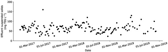
Figure 2.
The effluent suspended solids (ESS) concentrations, measured at the effluent weir in the settling tanks of the high rate activated sludge (HRAS) system under study (January 2017–November 2019).
2.2. Dispersed Suspended Solids Test
Mixed liquor samples were taken in the first section of the HRAS biological reactor and analyzed for DSS, according to the method described in Parker et al. [33]. Sampling and settling were performed in a single container with upper and lower closures (a 4.2 L Kemmerer sampler, with a diameter of 150 mm and a height of 600 mm). Using this single container spared biological flocs from any break-up or secondary flocculation effects resulting from intermediate transfer steps. The suspended solids (SS) analysis was performed according to the standard methods (Method 2540D [34]). Glass fiber filters with a pore size of 1.2 m and diameter of 70 mm were used for SS analyses of the supernatant. The DSS measure represented the current sludge flocculation state and could thus be considered as a reference standard to compare to the jar test results.
2.3. Jar Tests
A series of jar tests was performed simultaneously with the DSS test to investigate the effect of mixing before settling on the solids’ dispersion. The jar tests were performed in 124 mm square jars, for two different impeller types: an in-house made radial two blade paddle impeller (75 mm × 25 mm) and an axial three blade marine-type impeller (Heidolph Instruments, Germany) (diameter = 58 mm). The choice of the impeller sizes was based on those used in commercially available jar testers as no guidelines were available for AS flocculation tests. The jars were made of plexiglass with a liquid height of 130 mm. Figure 3 shows a schematic overview of the experimental setup. Square shaped jars were selected to avoid vortex flow during mixing [4]. It was visually observed that the minimum impeller speed to avoid dead zones (and thus solids settling) in the corners of the square jars was 30 and 70 rpm, for the radial and axial impeller, respectively. Mixing with an impeller speed below the latter limits did not provide enough kinetic energy to keep the solids in suspension. This is an unwanted effect in flocculation experiments [35]. Hence, impeller speeds below 30 and 70 rpm for, respectively, the radial and axial impeller were not considered in this study. A series of 6 jar tests was performed for the radial (30, 40, 50, 60, and 100 rpm) and axial impeller (70, 80, 100, 150, 250, 300). To achieve this, a large sludge sample (V = 12 L) was collected at the inlet of the aeration tank of the full scale HRAS system under study. The mixed liquor suspended solids (MLSS) concentration was determined according to the standard methods [34]. From the large sludge sample, six batches of 2 L were poured into six square jars, equipped with either the radial or axial impeller, and subjected to a specific impeller speed for 30 min. Subsequently, the mixed liquor was allowed to settle for 30 min. After the settling time elapsed, the supernatant was analyzed for SS.
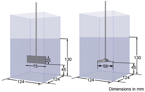
Figure 3.
Experimental setup of the jar test with a radial (left) and axial (right) mixer. The dimensions are in mm.
2.4. Particle Size Distribution
The particle size distribution (PSD) of several sludge samples was measured by image analysis with an Eye-Tech particle size analyser (Ankersmid, The Netherlands) before and after a jar test in order to investigate the mode and the degree of floc breakage. In this study, a lens with a measurement range of 10–600 was used to perform the image analysis. Due to the high solid concentrations, dilution was required to perform PSD analysis of the mixed liquor samples. The sludge was diluted with filtered effluent (disk filter of 0.45 ) to avoid disturbance of the floc structure (the dilution ratio was 1:100). The standard deviations on the PSD measurements were calculated based on at least 4 repetitions.
2.5. Computational Fluid Dynamics Modeling
CFD was used to predict the distribution of G in the two jar test setups (see Section 2.3) and in the anoxic section of the full scale HRAS system under study (see the description in Section 2.1). CFD modeling of stirred tanks is challenging since it requires careful selection of the grid resolution, impeller rotation model, physical models to describe turbulent transport, and numerical discretization schemes. These aspects impact considerably the computational expense and accuracy of the final results, and their selection has been an important point of discussion in many studies [21,23,24,36,37,38].
2.5.1. Steady State Model Development
For modeling of the impeller rotation, two main methodologies can be applied, depending on the level of detail or information required in the final results. The most accurate representation is the sliding mesh model. It simulates the unsteady flow field and interactions as they occur, but this comes with a high computational cost. The sliding mesh model is therefore only the preferred method in case interactions between rotor and baffles are strong (periodic, time dependent flow) and an accurate solution is desired [38]. An alternative methodology is the multiple reference frames (MRF) approach, which treats the essentially unsteady flow field around the impeller as a steady state at a given instant. It is similar to freezing the motion of the rotating impeller in a specific position and observing the flow field with the rotor in that position. This approach is computationally economic and has proven sufficiently accurate for steady state simulation of lab scale stirred tanks when compared to experimental data [36]. In the MRF approach, the computational domain needs to be subdivided into a rotating reference frame (related to the impeller zone) and a stationary reference frame (related to the outer region, including the rest of the tank). The momentum equation and closure models are resolved in the separate zones, and a steady state approximation is made in the zone interface. The effects of the blade rotation are accounted for by an extra term in the governing equations to reflect the virtual motion of the reference frame. The time averaged flow field and turbulence was solved using a steady state Reynolds averaged Navier–Stokes (RANS) solver for incompressible flows, the MRF impeller rotation model, and the standard k- turbulence model. This methodology yielded, from a practical point of view, the optimal balance between information gain and computational demand. Accurately capturing turbulence using the standard k- turbulence model is, however, a difficult task due to the inherent assumption of isotropic turbulence. Bridgeman et al. [21,28] studied swirling flows in a lab scale cylindrical baffled jar and found large deviations between laser Doppler anemometry (LDA) velocity measurements and CFD results in the regions next to and below the impeller, which was attributed to vortexing within the vessel. However, Deglon and Meyer [36] demonstrated that predictions can be improved by applying very fine grids and higher order discretization schemes. The latter modeling strategy was successfully applied for CFD modeling of lab scale cylindrical [36,37,39] and square [40,41] stirred vessels. The latter modeling strategy was also applied here. In the literature, there are only a few numerical studies of full scale hyperboloid shaped impellers [39]. In this work, the flow field generated by the hyperboloid impellers was simulated using a similar approach as the one used for the lab scale jar tests.
The steady state simulations were performed with the finite volume method in the CFD software OpenFOAM v6. A second-order discretization scheme was used for spatial discretization. The SIMPLE (semi-implicit method for pressure-linked equations) algorithm was used to solve the Navier–Stokes equations [42]. The pressure equation was solved using the geometric agglomerated algebraic multigrid (GAMG) solver, and a solver with Gauss–Seidel smoothing was used for the momentum equation and transport equations for turbulent quantities. Post-processing and visualization was performed in Paraview 5.6 and Python’s jupyter notebook.
2.5.2. CFD Model of the Jar Test
The three-dimensional geometries of the jar, radial impeller, and shaft were created in the software SALOME v9.2.1. The geometry of axial impeller was provided by Heidolp Instruments (Germany). For each configuration, the computational domains were discretized using an automatic meshing generator (SnappyHexMesh utility in OpenFOAM v6). A structured hexahedral grid was generated. The mesh was refined within the rotating frame to capture the impeller rotation adequately. Care was taken in the meshing procedure to ensure a relatively smooth transition between the rotating and stationary reference frame. Finally, a mesh was obtained of ∼1.8 and 3.0 million cells for the jar test equipped with the radial and axial impeller, respectively. Regarding the boundary conditions, the standard wall functions were employed on the tank walls, and the free liquid surface was treated as a wall with no shear to mimic the free surface behavior. The velocity field was initialized using the potentialFoam utility in OpenFOAM v6., which provides a conservative initial velocity field [43].
2.5.3. CFD Model of the Full Scale Mixers
The anoxic section of the full scale HRAS system was a rectangular channel (42 m in length, 4.2 m in width, and 6 m depth), containing 5 identical hyperboloid-shaped impellers with a diameter of 2.3 m, located 0.285 m above the bottom of the channel. The three-dimensional geometry of the HRAS channel was developed in SALOME v9.2.1 (see Figure 4). It should be noted that the geometry of the hyperboloid-shaped impellers was constructed based on simplified design drawings and pictures of the impeller, provided by the Water Board Brabantse Delta (the geometry was kept as realistic as possible, but the actual design details were not available due to confidentiality). The impeller shaft was not taken into account in the model, assuming that its impact on the flow field was minor compared to that of the impeller blades. The mesh was constructed using the snappyHexMesh utility in OpenFOAM v6. At the inlet, an inlet velocity (U = 0.2 ) was imposed, which was calculated based on the average inlet flow rate of the HRAS system under dry weather flow conditions. The turbulent dissipation rate () and the turbulent kinetic energy () at the inlet were set by specifying the turbulent mixing length and the turbulent intensity [43]. The velocity field was initialized using the potentialFoam utility. Standard wall functions were employed on the tank and impeller walls. The free surface was considered as a wall with no shear to mimic the free surface behavior. An outflow boundary condition was applied at the downstream outlet of the section.
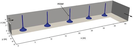
Figure 4.
3D model of the anoxic section of the full scale HRAS system at the water resource recovery facility (WRRF) Nieuwveer (Breda, NL).
The distribution of the local velocity gradients in the lab scale jar test and the full scale reactor was calculated via the concept of the local velocity gradient (G):
where P is the local power dissipated, V the reactor volume, the energy dissipation rate, and the kinematic viscosity.
3. Results and Discussion
3.1. Flocculation State of High Rate vs. Conventional Activated Sludge
The DSS values found for HRAS (122 ± 55 ) were considerably higher compared to those reported for CAS (<50 ) [7], indicating poor flocculation and settling characteristics. This can be attributed to the fact that the floc properties of the sludge produced in high rate systems are different compared to those in low rate systems. Figure 5 shows microscopic pictures of HRAS and CAS sludges, sampled at the WRRF Nieuwveer. In contrast to CAS sludge, which consisted of well flocculated particles, the HRAS sludge was composed of a combination of free living bacteria, small flocs (pinpoint-like flocs), and large amounts of fibers. These pinpoint-like flocs, containing little to no filaments, settled fast but had a reduced ability to act as a filter for fines. This could also be observed visually as the HRAS sludge settled clearly in two phases during the DSS test: within the first minutes, the bulk of solids settled very rapidly while a considerable fraction of the particles remained in the supernatant (no clear sludge blanket could be observed). The suspended particles that remained in the supernatant settled as discrete entities with lower settling velocities compared to the bulk. These small dispersed particles likely had a low separation efficiency in a settling tank and would also be captured less efficiently by air bubbles in DAF systems [44] or cause fouling and block the inner pores of membrane filtration units [45]. Incorporating more of these fines into flocs through optimization of the flocculation process would significantly improve the ESS concentrations in the HRAS system.
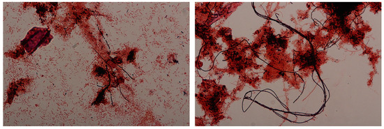
Figure 5.
Microscopy (magnified 630 times) of HRAS sludge (left) and conventional activated sludge (CAS) sludge (right), sampled in the first (HRAS process) and second stage (CAS process), respectively, at the WRRF Nieuwveer by Francis Meerburg.
3.2. Impact of Mixing on the Flocculation State
Figure 6 shows the supernatant SS concentrations after 30 min of settling, preceded by mixing in the square jars with either the radial or axial mixers and for different mixer speeds. It can be seen that subjecting the sludge to hydrodynamic shear prior to settling influenced the degree of SS that remained in the supernatant. This impact could only be attributed to a change in the sludge’s flocculation state induced by hydrodynamics shear since every series of jar tests, with either the radial or axial impeller (at different rpms), was performed at the same initial sludge concentration and the same initial flocculation state. For the radial impeller, a minimum supernatant SS concentration was reached by mixing with an impeller speed of 30 rpm. For the axial impeller, this occurred at 70 rpm. By slowly mixing the sludge with the radial impeller (30 rpm) before settling, the supernatant SS decreased by 54% and 21% compared to, respectively, the DSS and average ESS value. This significant decrease indicated that HRAS sludge had an excellent flocculation potential, but the current conditions in the full scale system and/or settling tank were not favorable for HRAS flocculation. Slowly mixing before settling likely increased the collision frequency between particles, resulting in an increased sweeping of small individual particles into the flocs. Furthermore, it can be seen that for the radial impeller the degree of SS in the supernatant increased rapidly with increasing impeller speed. It was hypothesized that the shear forces generated at higher impeller speeds were locally very high and shifted the equilibrium between floc aggregation and breakage more towards floc breakage.
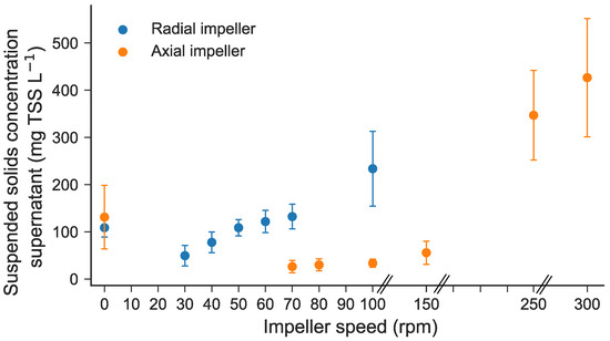
Figure 6.
The results of the dispersed suspended solids (DSS) tests (represented by the suspended solids (SS) concentrations at 0 rpm) and the jar tests, with either the radial or axial impeller and for different rpms. The SS concentrations show the averaged value based on five repetitions. The error bars represent the standard deviations. The mixed liquor suspended solids (MLSS) concentration of the raw sludge samples was 4.00 ± 0.73 .
Two different modes of floc breakage are described in literature: the erosion of small particles from the surface and floc rupture into two or more smaller flocs [33]. Previous researchers argued that floc erosion is more likely in CAS units than floc rupture because the extracellular polymeric substances (EPS) within the flocs are very much cross-linked. requiring high forces to break the floc [46]. However, the total amount of EPS and its composition in sludge flocs produced in HRAS systems is different, which influences its floc strength [16]. In order to make a distinction between floc erosion and fragmentation, Nopens et al. [47] investigated PSDs of sludge samples before and after mixing. This is however not straightforward for HRAS sludge due to two reasons: (1) the presence of a very broad range of particle sizes and (2) the fragile nature of HRAS sludge. Figure A1 (in Appendix A) shows examples of PSD measurements of HRAS sludge samples taken before and after mixing (for different impeller speeds). The presence of highly irregular flocs and large amounts of fibers in HRAS sludge disturbed the reliability of the measurements in the medium and large particle size classes, as manifested by the high standard deviations. An alternative strategy is to investigate the difference in the PSDs of the particles that remain in the supernatant after settling (see Figure A2). After 30 min, the majority of the large sized particles that disturbed the PSD were settled. It could be seen that increasing the impeller speed resulted in a larger fraction of small flocs (<50 m) in the supernatant. This indicated that the shear forces were large enough to break up the macro-flocs. However, primary particles in the range of 0.5–5 [48] were not measured by the apparatus as these were below the detection limit. For future research, it is therefore recommended to use a particle size analyzer with a very broad measurement range in order to quantify the degree of floc erosion.
In the case of the axial impeller, a different trend was observed. Mixing before settling yielded very low supernatant SS concentrations for an impeller speed up to 100 rpm. The average SS concentration in the supernatant was 31 ± 8 , which was, respectively, 75% and 51% lower than the DSS and average ESS value. The hydrodynamic conditions in the jar, generated by mixing with the axial impeller and impeller speeds up to 100 rpm, appeared to be more suitable for HRAS flocculation than those generated by the radial impeller. Although visually, no large differences in mixing between the axial and radial impeller could be observed, the results in Figure 6 indicated that the physical differences in the impeller type and speed had a significant influence on the supernatant SS concentrations and, hence, the (de)flocculation mechanism that prevailed. To further investigate this, information on the distribution of G in the jar is imperative.
3.3. Impact of Local Velocity Gradients
Figure 7 shows the contours of G in the midplane of the square jar, perpendicular to walls (x = 0), for the radial and axial impeller and for different impeller speeds. As expected, the distributions of the velocity gradient retrieved for the two impeller geometries were not uniform, with rather large differences in magnitude between the impeller region and the rest of the jar. At the same impeller speed, the reactor volume occupied by high velocity gradients was larger for the radial impeller compared to the axial impeller, which was important for floc breakage. The larger the reactor volume occupied by high velocity gradients, the more likely that floc breakage occurred. It could be seen that G values in the impeller region increased rapidly in magnitude and occupied a larger volume with increasing impeller speed, especially for the radial impeller. Mixing at 100 rpm with the radial impeller resulted in a large volume of local velocity gradients up to three times higher than the G value, which explained the high SS values found in the supernatant (see Figure 6). For the axial impeller, only a small volume was dominated by high velocity gradients.
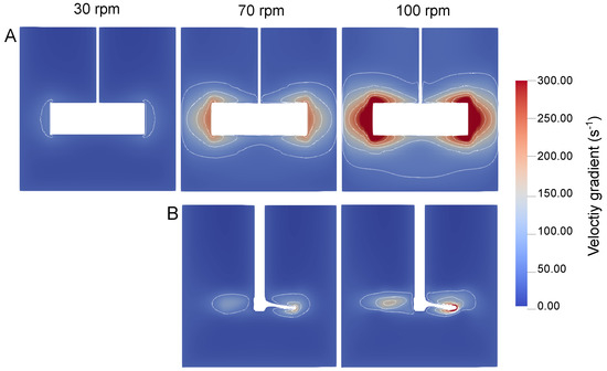
Figure 7.
Contours of local velocity gradients in a vertical plane (x = 0) of the jar, equipped with the radial (A) and the axial (B) mixers, for different impeller speeds.
To make a more detailed comparison, one could consider the distribution of the local velocity gradients not only in one plane (as shown in Figure 7), but in the whole jar volume [21]. Figure 8 displays the cumulative volume (%) distributions of G within the square jars, equipped with either the radial (dashed lines) or axial impeller (solids lines). The values of the average and maximum local velocity gradients (G and G) are summarized in Table 1. For the axial impeller, the value of G did not significantly change when the impeller speed was increased from 70 to 100 rpm. Its magnitude was in the same order as G obtained for the radial impeller at the lowest impeller speed (30 rpm). However, the distributions of local velocity gradients were significantly different, which may explain the differences found in supernatant SS concentrations (see Figure 6). The axial impeller produced very high G values (due to higher impeller speed) in its impeller region compared to the radial impeller, but these high velocity gradients were solely generated very locally in the near vicinity of the impeller blades. Indeed, from Figure 7, it can be seen that the distributions of G obtained for the axial impeller (70–100 rpm) were much steeper (i.e., more homogeneous), with a much lower volume (%) exhibiting high velocity gradients. The volume covered by high velocity gradients increased only marginally with increasing impeller speeds (in the case of the axial impeller) and likely did not result in increased floc breakage. The latter explained the low supernatant SS concentrations for an impeller speed up to 100 rpm in case of the axial impeller.
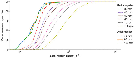
Figure 8.
The cumulative distribution of the local velocity gradients in the jar, equipped with the radial and the axial mixers, for different impeller speeds.

Table 1.
The average and maximum local velocity gradient (G and G), derived from the CFD simulations, for all jar test setups tested in this study.
The cumulative distributions obtained for the radial impeller were shifted to the right compared to those found for the axial impeller. The G distributions of the radial impeller were, hence, generally more dominated by higher velocity gradients compared to the axial impeller. Moreover, the volume occupied by high velocity gradients rapidly increased with impeller speed. Due to the fact that a radial impeller generates a flow perpendicular to the direction of the approaching sludge flocs, flocs change direction rapidly as they pass the impeller zone [3]. The flocs were therefore subjected to larger shear forces when passing the radial impeller compared to the axial impeller. A larger volume of high velocity gradients raised the likelihood of floc breakage to occur, as manifested by the higher supernatant SS by increased impeller speed (Figure 6). Bridgeman et al. [28] calculated the trajectory of neutrally buoyant spherical particles (500 in diameter) in a cylindrical jar (paddle impeller) for different impeller speeds. The latter author showed that flocs did not only experience higher G values with increasing impeller speed, but were also exposed more frequently to the peak G values in the impeller region. The latter phenomenon may explain the high increase in SS supernatant concentrations when the speed of the radial impeller was increased above 100 rpm.
The results above showed that the configuration of a jar test impacted the G distribution and, hence, the flocculation process of HRAS sludge, including the floc aggregation and breakage rates. In the standard FSS protocol, developed by Wahlberg et al. [4], it was assumed that mixing with an impeller speed of 50 rpm produces “ideal” flocculation conditions for AS flocculation. However, the optimal mixing speed may be different for different configurations of the jar test. The standard FSS protocol does not provide details regarding the impeller type and jar shape/size, and hence, the test should be re-evaluated and updated with appropriate recommendations on the jar test configuration. In this study, the flow distribution generated by the axial impeller appeared to promote better floc aggregation for HRAS sludge over a range of impeller speeds (up to 100 rpm) compared to the radial impeller as it produced a more homogeneous distribution of local velocity gradients.
Nevertheless, due to the wide distribution of the G within the jars, it was impossible to define a critical threshold beyond which floc breakage would occur. Repeating the flocculation experiments in a Taylor–Couette reactor could provide a solution here, as Coufort et al. [20] showed that the viscous dissipation of the turbulent kinetic energy in the latter vessel is quite uniform. Bridgeman et al. [21] stated that it was instructive to consider the range of G values obtained in a lab scale jar in which flocculation was promoted and compared those with values found in the full scale reactor. This model-based optimization strategy was more sound compared to solely considering average quantities and may help to understand and improve full-scale AS flocculation systems.
3.4. Comparison to a Full Scale Reactor
Figure 9 shows a comparison of the cumulative volume (%) distributions of G in the lab scale jars with those in the first part (anoxic section) of the full scale HRAS reactor at the WRRF Nieuwveer. For the full scale reactor, it can be seen that the values of the G were also not uniformly distributed. 90% of its volume exhibited very low local velocity gradients (<20 ). To further investigate the difference in the magnitude of G between the impeller region (i.e., in the first 2.5 m from the bottom of the tank) and the rest of the full scale channel (surface region), the distributions in the latter two regions are presented separately in Figure 9. The magnitude of the local velocity gradients in the impeller region of the full scale reactor was considerably larger than in the rest of the tank. In comparison to the lab scale jar (axial impeller), a rather large fraction of the volume (±8%) in the impeller region of the full scale mixers was occupied by high velocity gradients (>100 ). In these high shear zones, floc breakage may occur. In contrast, the region above the mixers (surface region) in the full scale reactor almost did not exhibit large local velocity gradients.
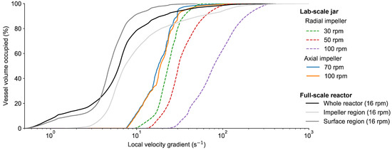
Figure 9.
Cumulative volume (%) distribution of the local velocity gradients (G) in the lab scale jar and in the first part (anoxic section) of the full scale HRAS system at the WRRF Nieuwveer.
3.5. Consequences for Flocculation Modeling
Combing experimental jar testing with CFD showed that for certain conditions, using a single number (G) to quantify the whole flow field in the jar would come with the risk of over- or under-estimating the actual shear stress to which the HRAS flocs are subjected. This was even more pronounced when moving to the full scale reactor. Over- or under-estimating hydrodynamic forces has important consequences for the prediction of the flocculation kinetics. Hence, potential distributions of the velocity gradients should not be overlooked when focusing on AS flocculation systems. Detailed information on the G distribution is necessary to fully comprehend and describe the aggregation and/or breakage rates of HRAS sludge in lab and full scale systems.
In order to study the flocculation state and the effects of aggregation and breakage in more detail, flocculation models can be used. It is still common practice to use flocculation models that are solely based on G. These models do not allow properly describing the dynamic equilibrium between floc aggregation and breakage and are not appropriate for the description of the HRAS flocculation behavior. A possible way to overcome these limitations is to couple the CFD model with a population balance model (PBM) that includes aggregation and break-up and, hence, can keep track of the dynamics of the sludge properties, such as the particle size. However, when considering particle size classes, this rapidly becomes very computationally demanding, especially for full scale systems. One solution is to rewrite the PBM in its moment form and only track moments (e.g., Marchisio et al. [49]). This, however, leads to the loss of accessibility to the PSD itself. Another option is to reduce the number of classes drastically (e.g., Lee et al. [50] or Ramalingam et al. [51]), but this also sacrifices accuracy. Yet another approach is to average aggregation and breakage rates over the volume domain (e.g., Castellano et al. [52]). A final strategy that can be used is to reduce the CFD model to a so-called compartmental model (CM) [53], before integration with a PBM. In this intermediate approach, the reactor volume is subdivided into a structural network of interconnected volumes in which the properties of the flow (e.g., the cumulative volume (%) distribution of velocity gradient) is assumed homogeneous. The CM used in conjunction with PBM can be used to describe the interaction between the dynamics of a floc property (e.g., size distribution) and one of the external influencing factors, i.e., turbulent shear. The increase in computational demand of a CM is marginal compared to a G model. Model calibration and validation are not so straightforward for these PBMs, but it is highly recommended to use these approaches instead of assuming an average shear value. The combination of such advanced modeling frameworks could greatly enhance our understanding of flocculation behavior and help in the development of optimization strategies for both the design and operation of HRAS systems.
4. Conclusions
In the present study, experimental and numerical data were combined to study the impact of local hydrodynamics on the flocculation performance of HRAS sludge in laboratory experiments and a full scale reactor. The main findings are as follows:
- The distribution of the velocity gradients within a jar test highly impacted the flocculation state of the sludge (and thus, the equilibrium between floc aggregation and breakage rates).
- The axial impeller appeared to be more appropriate for HRAS flocculation over a range of impeller speeds as it produced a more homogeneous distribution of local velocity gradients compared to the radial impeller.
- CFD is an excellent tool to acquire information on the distribution of local velocity gradients, which is necessary to describe the floc formation process of HRAS sludge accurately, including aggregation and breakage rates.
- Standard methods for flocculation jar tests should be updated with detailed information on the jar test configuration and appropriate recommendations for impeller type and velocity. A model based strategy can be used to link the information gained on lab scale to full scale systems.
Author Contributions
Conceptualization, all authors; methodology, S.B., S.E.V., U.R. and I.N.; software, S.B. and U.R.; validation, S.B., S.E.V. and I.N.; formal analysis, S.B. and L.Z.; investigation, S.B. and L.Z.; resources, S.E.V., L.H., L.Z. and I.N.; data curation, S.B. and I.N.; writing, original draft preparation, S.B., S.E.V., E.T., U.R. and I.N.; writing, review and editing, S.B., S.E.V., E.T., U.R. and I.N.; visualization, S.B.; supervision, S.B., S.E.V., E.T. and I.N.; project administration, S.B., L.H. and I.N.; funding acquisition, S.B., S.E.V., L.H. and I.N. All authors read and agreed to the published version of the manuscript.
Funding
This research was funded by Research Foundation Flanders (FWO SB Grant 1.S.705.18N).
Acknowledgments
The authors gratefully acknowledge the financial support of the Research Foundation Flanders (FWO SB Grant 1.S.705.18N). The authors thank the Water Board Brabantse Delta for their cooperation, support in experimental work, and participation in discussions. We thank Heidolp Instruments (Germany) for providing the 3D model of the axial impeller used in this work, Tinne De Boeck for the assistance with the experimental work, and Francis Meerburg for providing the microscopic pictures.
Conflicts of Interest
The authors declare no conflict of interest.
Appendix A

Figure A1.
Volume based (in %) particle size distributions (PSDs) of the sludge measured before and after 30 min of mixing (radial mixer) in a square jar, for different mixer speeds: (A) 30 rpm, (B) 50 rpm, and (C) 100 rpm. The standard deviations (SD) on the measurements are given by the shaded area (based on at least three repetitions).


Figure A2.
Volume based (in %) particle size distributions (PSDs) of the particles that stay behind in the supernatant after 30 min of settling, proceeded by 30 min of mixing (radial mixer) in a square jar with an impeller speed of 30 rpm, 50 rpm, or 100 rpm.
Figure A2.
Volume based (in %) particle size distributions (PSDs) of the particles that stay behind in the supernatant after 30 min of settling, proceeded by 30 min of mixing (radial mixer) in a square jar with an impeller speed of 30 rpm, 50 rpm, or 100 rpm.

References
- Spicer, P.T.; Pratsinis, S.E. Shear-induced flocculation: The evolution of floc structure and the shape of the size distribution at steady state. Water Res. 1996, 1354, 1049–1056. [Google Scholar] [CrossRef]
- Thomas, D.N.; Judd, S.J.; Fawcett, N. Flocculation modeling: A review. Water Res. 1999, 33, 1579–1592. [Google Scholar] [CrossRef]
- Spicer, P.; Keller, W.; Pratsinis, S. The Effect of Impeller Type on Floc Size and Structure during Shear-Induced Flocculation. J. Colloid Interface Sci. 1996, 184, 112–122. [Google Scholar] [CrossRef] [PubMed]
- Wahlberg, E.J.; Merrill, D.T.; Parker, D. Troubleshooting activated sludge secondary clarifier performance using simple diagnostic tests. In Proceedings of the 68th Annual WEF Conference and Exposition, Miami Beach, FL, USA, 21–25 October 1995; pp. 435–444. [Google Scholar]
- Moruzzi, R.B.; de Oliveira, A.L.; da Conceição, F.T.; Gregory, J.; Campos, L.C. Fractal dimension of large aggregates under different flocculation conditions. Sci. Total Environ. 2017, 609, 807–814. [Google Scholar] [CrossRef]
- Parker, D.; Butler, R.; Finger, R.; Fisher, R. Design and operations experience with flocculator-clarifiers in large plants. Water Sci. Technol. 1995, 33, 163–170. [Google Scholar] [CrossRef]
- Das, D.; Keinath, T.; Parker, D.; Wahlberg, E. Floc breakup in activated sludge plants. Water Environ. Res. 1993, 65, 138–145. [Google Scholar] [CrossRef]
- Khiewwijit, R.; Temmink, H.; Rijnaarts, H.; Keesman, K.J. Energy and nutrient recovery for municipal wastewater treatment: How to design a feasible plant layout? Environ. Model. Softw. 2015, 68, 156–165. [Google Scholar] [CrossRef]
- Böhnke, B. Das Adsorptions-Belebungsverfahrene. Korresp. Abwasser 1977, 24, 33–42. [Google Scholar]
- Jimenez, J.; Miller, M.; Bott, C.; Murthy, S.; De Clippeleir, H.; Wett, B. High-rate activated sludge system for carbon management-Evaluation of crucial process mechanisms and design parameters. Water Res. 2015, 87, 476–482. [Google Scholar] [CrossRef]
- Meerburg, F.; Van Winckel, T.; Vercamer, J.; Nopens, I.; Vlaeminck, S. Toward energy-neutral wastewater treatment: A high rate contact stabilization process to maximally recover sewage organics. Bioresour. Technol. 2015, 179, 373–381. [Google Scholar] [CrossRef]
- Liao, B.Q.; Droppo, I.G.; Leppard, G.G.; Liss, S.N. Effect of solids retention time on structure and characteristics of sludge flocs in sequencing batch reactors. Water Res. 2006, 40, 2583–2591. [Google Scholar] [CrossRef] [PubMed]
- Meerburg, F.; Vlaeminck, S.; Roume, H.; Seuntjens, D.; Pieper, D.H.; Jauregui, R.; Vilchez-Vargas, R.; Boon, N. High-rate activated sludge communities have a distinctly different structure compared to low-rate sludge communities, and are less sensitive towards environmental and operational variables. Water Res. 2016, 100, 137–145. [Google Scholar] [CrossRef] [PubMed]
- Mancell-egala, W.; Su, C.; Takacs, I.; Novak, J.; Kinnear, D.; Murthy, S.; De Clippeleir, H. Settling regimen transitions quantify solid separation limitations through correlation with floc size and shape. Water Res. 2017, 109, 54–68. [Google Scholar] [CrossRef]
- Agrawal, S.; Seuntjens, D.; De Cocker, P.; Lackner, S.; Vlaeminck, S.E. Success of mainstream partial nitritation/anammox demands integration of engineering, microbiome and modeling insights. Curr. Opin. Biotechnol. 2018, 50, 214–221. [Google Scholar] [CrossRef]
- Van Winckel, T.; Liu, X.; Vlaeminck, S.; Takács, I.; Al-Omari, A.; Sturm, B.; Kjellerup, B.; Murthy, S.; De Clippeleir, H. Overcoming floc formation limitations in high rate activated sludge systems. Chemosphere 2019, 215, 342–352. [Google Scholar] [CrossRef] [PubMed]
- Sancho, I.; Lopez-Palau, S.; Arespacochaga, N.; Cortina, J.L. New concepts on carbon redirection in wastewater treatment plants: A review. Sci Total Environ. 2019, 647, 1373–1384. [Google Scholar] [CrossRef] [PubMed]
- Camp, T.; Stein, P. Velocity gradients and internal work in fluid motion. J. Boston Soc. Civ. Eng. 1943, 30, 219–237. [Google Scholar]
- Bouyer, D.; Liné, A.; Do-Quang, Z. Experimental analysis of floc size distribution under different hydrodynamics in a mixing tank. AIChE J. 2004, 50, 2064–2081. [Google Scholar] [CrossRef]
- Coufort, C.; Bouyer, D.; Liné, A. Flocculation related to local hydrodynamics in a Taylor-Couette reactor and in a jar. Chem. Eng. Sci. 2005, 60, 2179–2192. [Google Scholar] [CrossRef]
- Bridgeman, J.; Jefferson, B.; Parsons, S. The development and application of CFD models for water treatment flocculators. Adv. Eng. Softw. 2010, 41, 99–109. [Google Scholar] [CrossRef]
- He, C.; Wood, J.; Marsalek, J.; Rochfort, Q. Using CFD Modeling to Improve the Inlet Hydraulics and Performance of a Storm-Water Clarifier. J. Environ. Eng. 2008, 134, 722–730. [Google Scholar] [CrossRef]
- Joshi, J.B.; Nere, N.K.; Rane, C.V.; Murthy, B.N.; Mathpati, C.S.; Patwardhan, A.W.; Ranade, V.V. CFD simulation of stirred tanks: Comparison of turbulence models (Part II: Axial flow impellers, multiple impellers and multiphase dispersions). Can. J. Chem. Eng. 2011, 89, 754–816. [Google Scholar] [CrossRef]
- Joshi, J.B.; Nere, N.K.; Rane, C.V.; Murthy, B.N.; Mathpati, C.S.; Patwardhan, A.W.; Ranade, V.V. CFD simulation of stirred tanks: Comparison of turbulence models. Part I: Radial flow impellers. Can. J. Chem. Eng. 2011, 89, 23–82. [Google Scholar] [CrossRef]
- Ducoste, J.J.; Clark, M.M.; Weetman, R.J. Turbulence in Flocculators: Effects of Tank Size and Impeller Type. AIChE J. 1997, 43, 328–338. [Google Scholar] [CrossRef]
- Coufort, C.; Dumas, C.; Bouyer, D.; Liné, A. Analysis of floc size distributions in a mixing tank. Chem. Eng. Process. Process Intensif. 2008, 47, 287–294. [Google Scholar] [CrossRef]
- Kilander, J.; Blomström, S.; Rasmuson, A. Scale-up behavior in stirred square flocculation tanks. Chem. Eng. Sci. 2007, 62, 1606–1618. [Google Scholar] [CrossRef]
- Bridgeman, J.; Jefferson, B.; Parsons, S. Assessing floc strength using CFD to improve organics removal. Chem. Eng. Res. Des. 2008, 86, 941–950. [Google Scholar] [CrossRef]
- Marshall, E.; Bakker, A. Computational Fluid Mixing. In Handbook of Industrial Mixing: Science and Practice; Paul, E.L., Atiemo-obeng, V.A., Kresta, S.M., Eds.; John Wiley & Sons Inc.: Hoboken, NJ, USA, 2004; pp. 257–343. [Google Scholar] [CrossRef]
- Oyegbile, B.; Ay, P.; Narra, S. Flocculation kinetics and hydrodynamic interactions in natural and engineered flow systems: A review. Environ. Eng. Res. 2016, 21, 1–14. [Google Scholar] [CrossRef]
- De Graaff, M.S.; van den Brand, T.P.; Roest, K.; Zandvoort, M.H.; Duin, O.; van Loosdrecht, M.C. Full-Scale Highly-Loaded Wastewater Treatment Processes (A-Stage) to Increase Energy Production from Wastewater: Performance and Design Guidelines. Environ. Eng. Sci. 2016, 33, 571–577. [Google Scholar] [CrossRef]
- Seuntjens, D.; Bundervoet, B.L.; Mollen, H.; De Mulder, C.; Wypkema, E.; Verliefde, A.; Nopens, I.; Colsen, J.G.; Vlaeminck, S.E. Energy efficient treatment of A-stage effluent: Pilot scale experiences with shortcut nitrogen removal. Water Sci. Technol. 2016, 73, 2150–2158. [Google Scholar] [CrossRef]
- Parker, D.; Kaufman, W.; Jenkins, D. Characteristics of Biological Flocs in Turbulent Regime; Technical Report; University of California: Berkeley, CA, USA, 1970. [Google Scholar]
- APHA. Standard Methods for the Examination of Water and Wastewater, 22nd ed.; American Public Health Association: Washington, DC, USA; American Water Works Association: Washington, DC, USA; Water Environment Federation: Washington, DC, USA, 2012; p. 1496. [Google Scholar]
- Torfs, E.; Nopens, I.; Winkler, M.K.; Vanrolleghem, P.A.; Balemans, S.; Smets, I.Y. Settling tests. In Experimental Methods in Wastewater Treatment; van Loosdrecht, M., Nielsen, P., Lopez-Vazquez, C.M., Brdjanovic, D., Eds.; IWA Publishing: London, UK, 2016; pp. 235–262. [Google Scholar]
- Deglon, D.A.; Meyer, C.J. CFD modeling of stirred tanks: Numerical considerations. Min. Eng. 2006, 19, 1059–1068. [Google Scholar] [CrossRef]
- Aubin, J.; Fletcher, D.F.; Xuereb, C. Modeling turbulent flow in stirred tanks with CFD: The influence of the modeling approach, turbulence model and numerical scheme. Exp. Therm. Fluid Sci. 2004, 28, 431–445. [Google Scholar] [CrossRef]
- Bridgeman, J.; Jefferson, B.; Parsons, S.A. Computational Fluid Dynamics modeling of flocculation in water treatment: A review. Eng. Appl. Comput. Fluid Mech. 2009, 3, 220–241. [Google Scholar]
- Alleyne, A.A.; Xanthos, S.; Ramalingam, K.; Temel, K.; Li, H.; Tang, H.S. Numerical investigation on flow generated by invent mixer in full scale wastewater stirred tank. Eng. Appl. Comput. Fluid Mech. 2014, 8, 503–517. [Google Scholar] [CrossRef]
- He, W.; Xue, L.; Gorczyca, B.; Nan, J.; Shi, Z. Comparative analysis on flocculation performance in unbaffled square stirred tanks with different height-to-width ratios: Experimental and CFD investigations. Chem. Eng. Res. Des. 2018, 132, 518–535. [Google Scholar] [CrossRef]
- He, W.; Xue, L.; Gorczyca, B.; Nan, J.; Shi, Z. Experimental and CFD studies of floc growth dependence on baffle width in square stirred-tank reactors for flocculation. Sep. Purif. Technol. 2018, 190, 228–242. [Google Scholar] [CrossRef]
- Versteeg, H.K.; Malalasekera, W. An introduction to Computational Fluid Dynamics: The Finite Volume Method, 2nd ed.; Pearson Education Limited: Essex, UK, 2007; p. 520. [Google Scholar]
- Greenshields, C.J. The OpenFOAM Foundation User Guide 7.0; The OpenFOAM Foundation Ltd.: London, UK, 10 July 2019. [Google Scholar]
- Cagnetta, C.; Saerens, B.; Meerburg, F.A.; Decru, S.O.; Broeders, E.; Menkveld, W.; Vandekerckhove, T.G.; De Vrieze, J.; Vlaeminck, S.E.; Verliefde, A.R.; et al. High-rate activated sludge systems combined with dissolved air flotation enable effective organics removal and recovery. Bioresour. Technol. 2019, 291. [Google Scholar] [CrossRef]
- Faust, L.; Temmink, H.; Zwijnenburg, A.; Kemperman, A.J.B.; Rijnaarts, H.H.M. High loaded MBRs for organic matter recovery fromsewage: Effect of solids retention time on bioflocculation and on the role of extracellular polymers. Water Res. 2014, 56, 258–266. [Google Scholar] [CrossRef]
- Mikkelsen, L.H. The shear sensitivity of activated sludge: Relations to filterability, rheology and surface chemistry. J. Colloid Interface Sci. 2001, 182, 1–14. [Google Scholar]
- Nopens, I.; Biggs, C.; De Clercq, B.; Govoreanu, R.G.; Wilén, B.; Lant, P.; Vanrolleghem, P. Modelling the activated sludge flocculation process combining laser diffraction particle sizing and population balance modeling (PBM). Water Sci. Technol. 2002, 45, 41–49. [Google Scholar] [CrossRef]
- Li, D.H.; Ganczarczyk, J.J. Size distribution of activated sludge flocs. Res. J. Water Pollut. Control Fed. 1991, 63, 806–814. [Google Scholar]
- Marchisio, D.L.; Vigil, R.D.; Fox, R.O. Quadrature method of moments for aggregation-breakage processes. J. Colloid Interface Sci. 2003, 258, 322–334. [Google Scholar] [CrossRef]
- Lee, B.J.; Toorman, E.; Molz, F.J.; Wang, J. A two-class population balance equation yielding bimodal flocculation of marine or estuarine sediments. Water Res. 2011, 45, 2131–2145. [Google Scholar] [CrossRef] [PubMed]
- Ramalingam, K.; Xanthos, S.; Gong, M.; Fillos, J.; Beckmann, K.; Deur, A.; McCorquodale, J.A. Critical modeling parameters identified for 3D CFD modeling of rectangular final settling tanks for New York City wastewater treatment plants. Water Sci. Technol. 2012, 65, 1087–1094. [Google Scholar] [CrossRef] [PubMed]
- Castellano, S.; Sheibat-Othman, N.; Marchisio, D.; Buffo, A.; Charton, S. Description of droplet coalescence and breakup in emulsions through a homogeneous population balance model. Chem. Eng. J. 2018, 354, 1197–1207. [Google Scholar] [CrossRef]
- Rehman, U. Next Generation Bioreactor Models for Wastewater Treatment Systems by Means of Detailed Combined Modelling of Mixing and Biokinetics. Ph.D. Thesis, Ghent University, Ghent, Belgium, 2016. [Google Scholar]


© 2020 by the authors. Licensee MDPI, Basel, Switzerland. This article is an open access article distributed under the terms and conditions of the Creative Commons Attribution (CC BY) license (http://creativecommons.org/licenses/by/4.0/).