Permeate Flux Control in SMBR System by Using Neural Network Internal Model Control

Abstract

This paper presents a design of a data-driven-based neural network internal model control for a submerged membrane bioreactor (SMBR) with hollow fiber for microfiltration. The experiment design is performed for measurement of physical parameters from an actuator input (permeate pump voltage), which gives the information (outputs) of permeate flux and trans-membrane pressure (TMP). The palm oil mill effluent is used as an influent preparation to depict fouling phenomenon in the membrane filtration process. From the experiment, membrane fouling potential is observed from flux decline pattern, with a rapid increment of TMP (above 200 mbar). Membrane fouling is a complex process and the available models in literature are not designed for control system (filtration performance). Therefore, this work proposes an aeration fouling control strategy to measure the filtration performance. The artificial neural networks (Feed-Forward Neural Network—FFNN, Radial Basis Function Neural Network—RBFNN and Nonlinear Autoregressive Exogenous Neural Network—NARXNN) are used to model dynamic behaviour of flux and TMP. In this case, only flux is used in closed loop control application, whereby the TMP effect is used for monitoring. The simulation results show that reliable prediction of membrane fouling potential is obtained. It can be observed that almost all the artificial neural network (ANN) models have similar shape with the actual data set, with the highest accuracy of more than 90% for both RBFNN and NARXN. The RBFNN is preferable due to simple structure of the network. In the control system, the RBFNN IMC depicts the highest closed loop performance with only 3.75 s (settling time) for setpoint changes when compared with other controllers. In addition, it showed fast performance in disturbance rejection with less overshoot. In conclusion, among the different neural network tested configurations the one based on radial basis function provides the best performance with respect to prediction as well as control performance.

1. Introduction

Membrane Bioreactor (MBR) technology has become one of the most popular mechanisms of filtration systems and has become a necessity in wastewater treatment technology. High concerns about environmental pollution and the stringent requirement of effluent make this technology gain more attention worldwide. MBR is one of the best alternative technologies that are used to replace Conventional Activated Sludge (CAS). Many advantages have been discovered by using MBR over conventional technologies including CAS [1]. This technology is proven to be efficient in producing high-quality effluents for domestic and industrial wastewater treatments [2,3,4]. The MBR system consists of two main processes, which are biological and filtration parts. The most critical part of any MBR system is the membrane filtration process. The successful operation of the MBR depends on the performance of the membrane filtration. The main issue of MBR is its filtration process is complex and hard to model. Fouling is a major problem in the membrane filtration system [4,5,6,7]. It can be categorized as unwanted accumulation of substances such as colloidal, particulate, solute material, and microorganism on the membrane during the filtration process [8]. Membrane fouling contributes to the deposition of sludge cake and pore-clogging that prompt to membrane damage [9]. This phenomenon will cause a rapid increment in trans-membrane pressure (TMP) and increase in hydraulic resistance during the filtration process and hence reduce the permeate flux. The development of control filtration system is crucial in order to prevent or at least delay the replacement of the membrane module.

In a filtration control system, a reliable prediction model is important to improve the performance of the MBR plant [10]. The membrane filtration process requires a good model and control to produce an efficient filtration system. A model-based control technique is an alternative to produce better control performance. However, this method requires a high degree of model accuracy to ensure the controller is at the desired performance. Artificial neural network (ANN), also called intelligence modeling, is among the most popular algorithms for modeling of membrane filtration systems [10]. The Radial Basis Function Neural Network (RBFNN), multilayer perceptron neural network, and general regression neural network model structures are widely utilized in filtration modeling of synthetic wastewater treatment [11]. Good predictions of membrane fouling potential profile were obtained using the model structures. The ability of the RBFNN method to predict the interfacial interactions with the randomly rough membrane surface has been presented in [12,13]. In addition, the method has shown a wide potential of membrane fouling and interface behavior applications. Therefore, it is envisaged that the RBFNN could pave a new way for modelling of membrane fouling in MBRs. Bagheri et al. [14] developed two types of feed-forward artificial networks which are multilayer perceptron and radial basis function. Both types of radial basis function and multilayer perceptron are chosen because of their ability to deal with nonlinear relationships in the data.

Radial basis function and multi-layer perceptron are two types of artificial neural networks, which are most commonly used in classification problems [15,16]. The RBFNN has the advantages of adaptation capability, robust ability, learning stage without any iteration of updating weights, and very fast learning process [17]. It is widely used in variety of applications and effectively solved many control problems [17,18,19]. In addition, its structure is simple and more important is able to approximate any nonlinear function [19]. Giwa et al. [20] introduced a new configuration of an electrically-enhanced membrane bioreactor to treat medium-strength wastewater at Masdar City, Abu Dhabi, United Arab Emirates. An artificial neural network-based ensemble model was utilized to model the experimental findings of chemical oxygen demand, orthophosphates, and ammonium nitrogen removal given the initially mixed liquor characteristics. The ANN model result and experimental data set gave high correlation coefficients. Internal Model Control (IMC) is one of the potential control methods that has received much attention from researchers in process control industries. The prevalence of the internal model control strategy is primarily due to its simple tuning parameter, good disturbance rejection, and robustness [21,22]. In addition, the simplicity and effectiveness of the IMC controller for disturbance rejection and closed loop performance make it the best chosen control structure for this system [23]. Despite these advantages, IMC still faces limitations for systems with highly nonlinear dynamics [23]. The effectiveness of the IMC depends on how good the model captures accurately the dynamic behavior of the system.

A good model of the system is a key simplifying design and implementation of the membrane filtration control system. Several nonlinear IMC strategies have been proposed by previous literature in variety of applications [24,25,26]. The nonlinear IMC control methods implemented are based on the conventional IMC that faced with the limitation of disturbances entering the process before control action is taken.

For an ANN-based IMC control method, ANN is trained to learn the inverse dynamics of the process and employed as a nonlinear controller. The IMC can perform efficiently if the actual plant and plant model matched exactly. The combination of ANN and IMC is proven to provide good performance of the control system. For example, the Neural Network Internal Model Control (NNIMC) is developed to control the top and bottom composition in the distillation column for set point and disturbance rejection performance analysis [27]. The result shows NNIMC provides better performance which is more robust and stable when compared to the conventional proportional-integral plus feed-forward controller. Sun et al. [28] proposed the neural network inverse scheme and 2-degree-of-freedom internal model control and improve the tracking and disturbance rejection performances. In the application of inverted pendulum system [29], IMC was designed using the inverse of the plant model and showed better response specifications when compared with the conventional Proportional-Integral-Derivative controller. The simulation results also demonstrate the robustness of the IMC. The ANN-based IMC is also depicted in the application of wastewater treatment plant [30]. In this new ANN-based IMC, the control performance was improved in which reduced the performance degradation.

This paper presents an NNIMC-based control of membrane bioreactor filtration process, with submerged hollow fiber installed inside the tank. In order to retain the great advantage offered by an ANN and the IMC, the NNIMC is proposed to control the permeate flux and TMP of membrane bioreactor. The accuracy of the model is established by comparing three different ANN models (Feed-Forward Neural Network—FFNN, RBFNN and Nonlinear Autoregressive Exogenous Neural Network—NARXNN) to achieve an accurate prediction of dynamic (fouling) behaviour. The NNIMC control structure is improved with the additional filter design to minimize the effect of model mismatch and hence provide better performance of the control system.

The main contributions of this work can be summarized as:

(a)

To the best of authors’ knowledge, this is the first work on designing an NNIMC controller for a submerged membrane bioreactor process, considering the flux and TMP effects at permeate stage, in order to predict the behaviour of fouling process.

(b)

Experimental work is performed to obtain the real input-output data of membrane filtration process that can be used for prediction of fouling phenomenon. The experimental design of the submerged MBR is performed using critical flux test, in order to determine the optimal flux before the pressure jump, which is closely related to the fouling development on membrane process

(c)

The accuracy of the developed model is analyzed, and this is used to investigate the performance of the controller.

(d)

The NNIMC controller is designed, such that to predict the plant behaviour under any circumstances such as disturbance and set point change, to prevent flux decline in the membrane filtration cycle due to fouling problem. In addition, an ANN shows good prediction when dealing with complicated processes like fouling phenomenon.

2. Research Methodology

The successful operation of a membrane filtration of wastewater treatment plant depends on the accuracy of the models for control system developments. Fouling is the main challenge in the filtration control system. This is caused by the blockage of the membrane pores due to impurities in the raw Palm Oil Mill Effluent (POME). This section presents the methodology of neural network model development and internal model control for Submerged Membrane Bioreactor (SMBR) filtration process. There are several steps in modelling the process which start with data collection, followed by model structure selection, parameter estimation and model validation. In this work, three different ANN architectures are used for modeling of membrane filtration process. They are Feed-Forward Neural Network (FFNN), RBFNN and Nonlinear Autoregressive Exogenous Neural Network (NARXNN) architectures. The permeated pump voltage is an input and the outputs are permeated flux and transmembrane pressure of filtration processes. The accuracy of models is determined based on three performance criteria that are correlation coefficient R², Mean Square Error (MSE) and Mean Absolute Deviation (MAD), which later applied for Neural Network Internal Model Control (NNIMC) to control fouling development in the membrane filtration process. The performance evaluation of the controller is measured using rise time, settling time, overshoot, Integrated Absolute Error (IAE), Integrated Time Absolute Error (ITAE) and Integrated Squared Error (ISE). The simulation studies were carried out using MATLAB software. The details of the flow of methodology are depicted in Figure 1.

2.1. Data Collection and Analysis

The experiments of the SMBR pilot plant were set up. The plant consisted of a single bioreactor tank with submerged hollow fiber installed inside the tank. The hollow fiber membrane (with three membrane modules) was fabricated at Advance Membrane Technology Centre (AMTEC UTM) using polyethersulfone (PES) material ultrafiltration with approximately in range of pore size of 800–1000 kda or 0.05–0.09 µm.

The POME with a volume of 20 L was taken from Sedenak Palm Oil Mill Sdn. Bhd. Johor, Malaysia. The plant was subjected to sustained input changes. Such changes can be approximated by a step function which is given by Equation (1).

$$u\left(t\right)= \{\begin{array}{c}0 t=t_{relaxation}\\ u_A t=t_{permeate}\end{array}$$

(1)

where $u_A$ is the desired amplitude. The plant will be OFF for $t=t_{relaxation}$. When t = $t_{permeate}$, the function will drive the system up to $u_A$. In this work, the plant was operated with continuous aeration airflow with alternate permeate and relaxation modes: a period of 120 s in permeation mode followed by 30 s in relaxation mode. The backwash process was performed at the beginning of the experiment for a period of 5 s. The backwash flow rate was not measured in this work, however the TMP was monitored not to reach more than 500 mbar. To keep the membrane at high performance, a high intensity of bubble flow is required. Therefore, in this filtration process, the aeration airflow was set around 6 to 8 LPM. The temperatures of working for the bioreactors were at 27 ± 1 °C. The pilot plant consisted of four streams including inlet stream, aeration stream, permeate stream, and backwash stream. The data plant was controlled and monitored using LabVIEW 2009 software, National Instruments, with NI USB 6009 interfacing hardware. 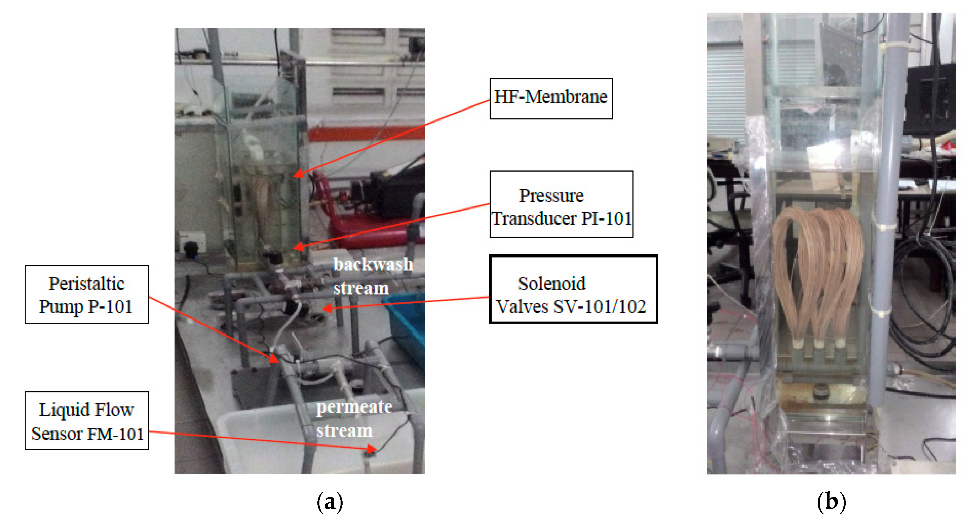Figure 2 shows the schematic diagram of the SMBR pilot plant set up for the experiment and Figure 3a,b present the actual developed SMBR.

The data collection was performed using the actual SMBR pilot plant shown in Figure 3a while Figure 3b presents the close view of three membrane modules of HF-membrane. The permeate stream and backwash stream are shown in Figure 3a. The filtered effluent from the HF-Membrane Bioreactor was pumped using a peristaltic pump (P-101) and the solenoid valve (SV 101) was opened during permeate stage. The permeate flux and TMP outputs were measured using electronic flow sensor (FM 101) and electronic pressure transducer (PI-101), respectively. To clean the membrane, a backwash process was applied. The backwash process was performed at the beginning of the experiment for a period of 5 s. During backwash, the P-102 backwash pump and the solenoid valve (SV 102) were activated to allow filtered tap (clean) water in the backwash storage tank to flow in and clean the membrane. The preliminary study was conducted to select the best operational control strategies to reduce fouling phenomenon that are; (a). aeration airflow process, (b). backwash operation and (c). relaxation operation. In this work, permeate to relaxation ratio operation is set in every cycle of operation (120:30). The backwash mechanism was applied at the beginning of the experiment for 5 s, not for every cycle of operation. The relaxation test was conducted to obtain an optimum relaxation time. With the filtration cycle of 120 s, the relaxation was varied between 10, 20 and 30 s. The experiment study showed that no significant different for TMP increment was observed at first 30 cycle. However, the 10 s relaxation showed high measurement of TMP after 30 cycle of the experiment when compared with the relaxation at 20 and 30 s. After 50 cycles of the experiment, the 30 s relaxation showed a slower TMP increment compared to 20 s relaxation. From observation, longer relaxation gave a slower TMP increment, however a too long relaxation period reduced the permeation flux. The ideal relaxation period used in this work was 30 s. In future work, the combination of the relaxation and the backwash techniques could be considered.

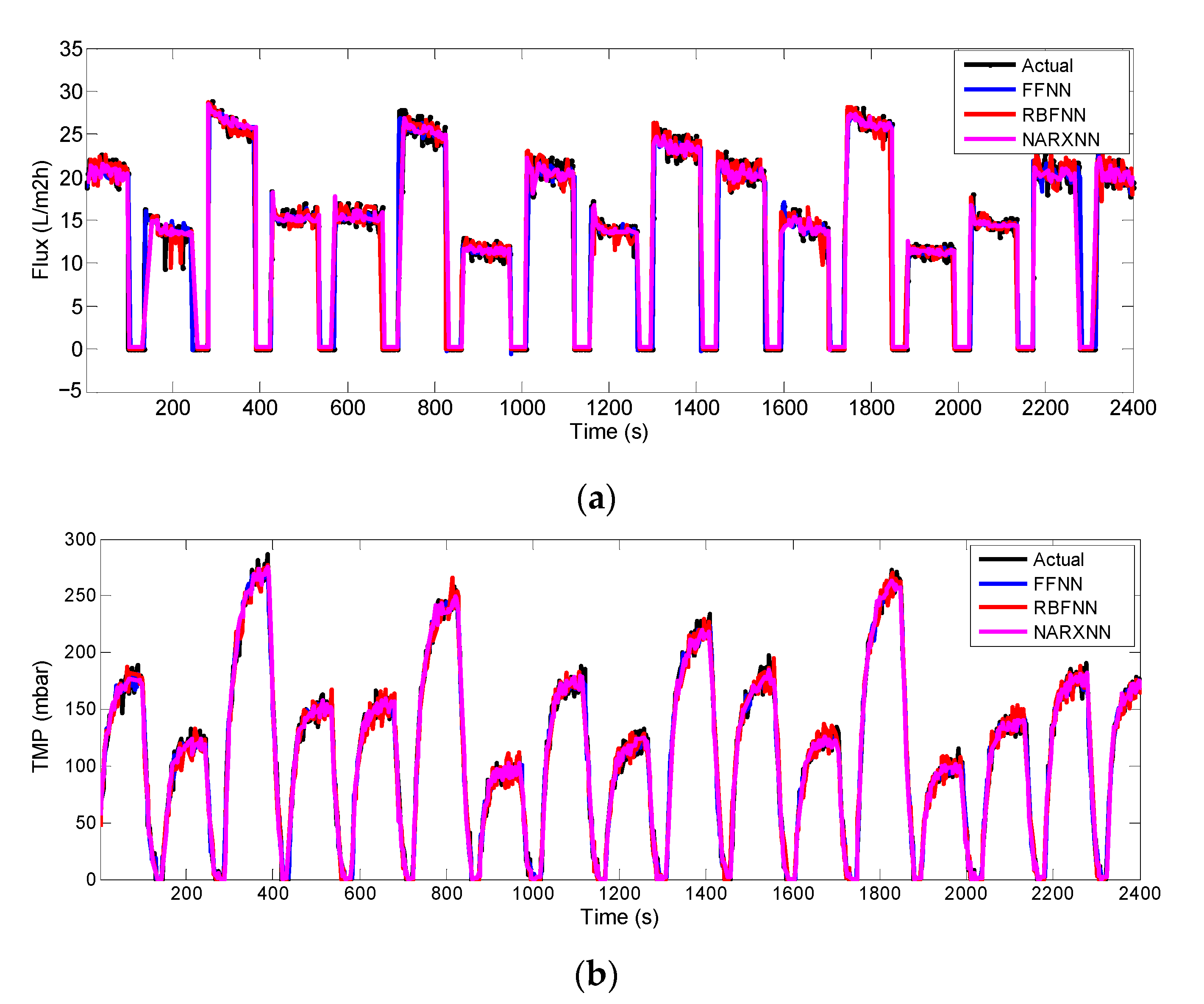
The excitation of the input is crucial in order to ensure good dynamic behavior of the filtration process can be obtained. The permeate pump voltage represents an input while the flux and TMP are the outputs of the plant. In this experimental work, random magnitude of step inputs was excited into the suction pump. The obtained input–output data set for SMBR filtration process is presented in Figure 4. It can be observed from the figure that the changes of the permeate pump voltage setting had an effect on both permeate flux and TMP as system outputs. As can be observed from Figure 4. In addition, the flux showed a declined pattern for a rapid increment of TMP, in particular above 200 mbar. This pressure jump occurred because the membrane was totally blocked by the undesired particular substance (cake resistance fouling). Therefore, it was important to ensure the filtration operation was performed below the critical flux, in order to prevent rapid fouling and improve the performance of membrane filtration process.

2.2. Data Pre-Processing

The second flow of modelling was data pre-processing. Data pre-processing included data normalization and data division. Generally, there is a need for the data pre-processing to transform the collected data into understandable format. Real data usually needs some preprocessing for minimizing eventual errors that may occur during data acquisition. In addition to range accommodation, there may be missing values for some of the variables, noise, etc. In this study, the data were set to an appropriate range for ANN learning in the model development.

2.2.1. Data Normalization

Data normalization or also known as scaling is very important before applying ANN to model MBR filtration process. The normalization of the data is to prevent attributes with a large numeric scale from dominating those in small scale. This also helps to simplify the difficulties during the calculation. This process minimizes the chances of overflows and underflows of data. Normally, normalized data can be scaled into the range [−1, +1] or [0, 1]. It is recommended to scale the data before the process of training and testing begins. In this work, the dataset was scaled in the range of (0, 1). Equation (2) was used to normalize the data as follows:

$$x=\frac{\left(MaxVal-MinVal\right)}{d_{max}-d_{min}}\left(d_i-d_{min}\right)+MinVal$$

(2)

where d_i is the ith input–output data, d_max is the maximum value of input-output data and d_min is the minimum value of the input–output data.

2.2.2. Data Division

Data division is the division of the whole data set into two sets of data that are training and testing data sets. Training data sets are used as an input training in order for the ANN to obtain the model/pattern. The testing dataset is used as input testing that will be used to obtain the prediction output/value. According to [2], no specific rule is needed to determine the data division of training and testing dataset. For this system, the training dataset should be more than 50% from the whole experimental dataset to ensure the reliability of the model. In this work, the data set was divided into 60% (2400 samples) for the training and 40% (1600 samples) used for testing.

2.3. Performance Evaluation

The prediction accuracies of the realized models were evaluated using standard measurement of performance indexes that are Mean Square Error (MSE), Mean Absolute Deviation (MAD) and correlation coefficient, R².

i.

Mean square error (MSE)

MSE measures the difference between the observed values and estimated values by a model. Mathematically, MSE is expressed as:

$$MSE=\frac{{\displaystyle \sum |{\widehat{y}}_i-{y_i|}^2}}{N}$$

(3)

where ${\widehat{y}}_i$ is the observed value, $y_i$ is the predicted value, and N is the number of data.

ii.

Mean absolute deviation (MAD)

MAD is one of the easiest and most popular measures for evaluating performance of the model [31]. MAD is the average of the discrepancy between the estimated and measured values, given by the following expression

$$MAD=\frac{{\displaystyle \sum |w_i-{{\widehat{w}}_i|}^{}}}{N}$$

(4)

where wᵢ is the predicted value, ŵᵢ is the mean of the predicted value and N is the number of data.

iii.

Correlation Coefficient (R²)

Correlation coefficient measures the strength of similarity between two variables. Correlation coefficient is given by:

$$R^2={(\frac{{\sum }_{i=1}^N\left(w_i-\widehat{w}\right)\left(y_i-\widehat{y}\right)}{\sqrt{({\sum }_{i=1}^N{\left(w_i-\widehat{w}\right)}^2)({\sum }_{i=1}^N{\left(y_i-\widehat{y}\right)}^2)}})}^2$$

(5)

where wᵢ is the measured value, ŵ is mean of the measured value, yᵢ is the predicted value, ŷ is mean of the predicted value and N is the number of data.

2.4. Modelling of ANN

In this work, the data was divided into 60% for the training and 40% used for testing. After selecting the learning algorithm, the number of training epochs was chosen in order to train the ANN model. After obtaining the desired model, the model was examined to predict the unknow data (testing data). This could reveal the generalization capability of the model. The modelling techniques for each one of the three ANN structures are explained in what follows.

2.4.1. Feed-Forward Neural Network Method

The SMBR filtration data set (4000 data samples) was utilized to develop the model. The measured data were normalized as per (2), so that the data values were between zero (0) and one (1). Data normalization helps neural network training by getting a faster convergence as well as by minimizing the risk of getting stuck in local minima [32]. Data pre-processing is an important procedure in model development (neural network model). This will ensure the efficiency of the data processing and the reliability of the model. Data normalization (or called magnitude scaling) in this work means to rescale the input and output data from 0 to 1. This step allows improvement on the numerical processing convergent time [33].

The normalized data were divided into 60% (2400 samples) for the training and 40% (1600 samples) used for testing the model. The determination of the structure for the FFNN was crucial and required more effort to accomplish. In this paper, the network structure was selected considering the relationship proposed in [23].

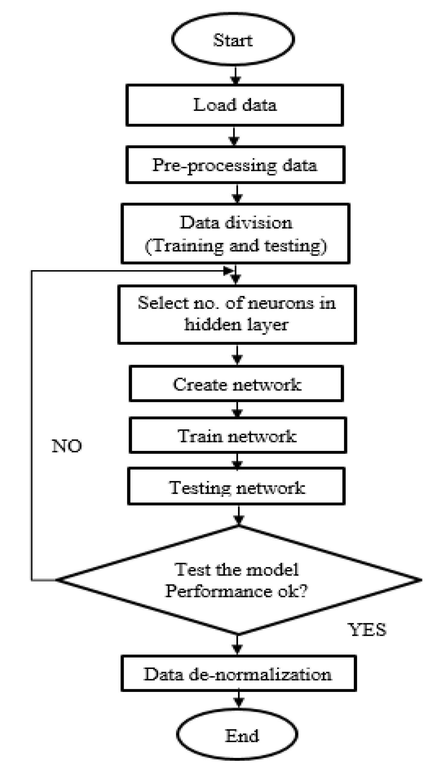
The FFNN structure comprises three layers including input layer, hidden layer and the output layer. The determination of number of neurons in the hidden layer is critical for effective learning and performance. In this work, the FFNN structure was varied from 1 to 10 hidden neurons and the performance was measured using MSE criteria. For each number of hidden neurons, the training was repeated eight times to determine the best, average, and worst performances. The process weights were first initialized to small random numbers prior to the training. The weights were adjusted till the error for the entire set was acceptably low before the training was terminated. In this work, the simulation results showed that the MSE for five hidden layer neurons with 10 weights for flux output, and seven hidden layer neurons with 14 weights for TMP output, gaves the best performance.

For the feed-forward neural network, the tan-sigmoid transfer function was employed for the hidden layer and linear weights for the output layer. The backpropagation was used for the network training of 1000 epochs as the set stooping criteria. Then, the FFNN model was provided with the testing data once the training stage was stopped. To ensure good prediction of models, the performance criteria using MSE, MAD, and R² were performed. The procedure of developing the FFNN is described in Figure 5.

2.4.2. Radial Basis Function Neural Network Method

The SMBR filtration data set was also used to develop the RBFNN model. The same procedure applied as in the FFNN for normalization of the data, choice of the training and testing data were applied in the RBFNN modelling. The normalization allowed the data to be transformed into trainable and convenient for the network learning. Furthermore, it made training faster and reduces the chances of duplication of data. The RBFNN structure consisted of three layers which were the input layer, hidden layer and the output layer. Choosing the number of neurons in the hidden layer is very crucial for effective learning and performance. In this work, the ANN structure was varied from 1 to 10 hidden neurons and the performance was measured using MSE, MAD, and R². For each number of hidden neurons, the training was repeated eight times to determine the best, average, and worst performances.

For RBFNN, the activation function depends on the best optimized center and the radial distance between input layer to the hidden layer and the output layer to the hidden layer as shown in Figure 6.

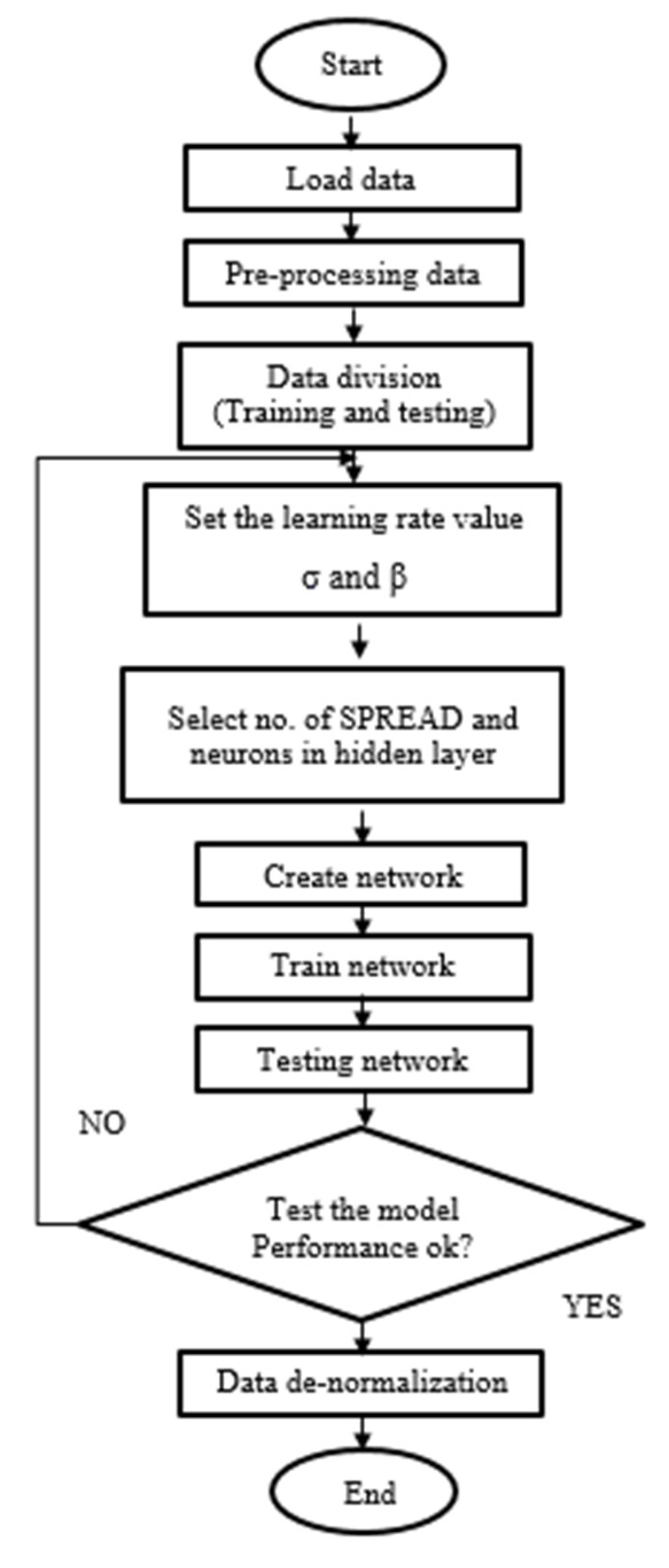
The adjustment of weight was carried out by selecting suitable learning rate values as well as spread values. Such spread value provides a measure of the sensitivity to input data. The larger the spread, the less the sensitivity of the radial. Two different learning rate values are used for each hidden layer and output layer. The learning rate, σ is used for hidden layer while the output layer uses learning rate, β. The best values of σ and β were given as σ = 10 and β = 5 for flux output while σ = 8 and β = 3 for TMP output. In order to effectively analyze the spread value with respect to hidden neuron, the number of hidden neurons is varied. In this work, it was varied from 1 to 10 hidden neurons. The spread value was selected based on the MSE criteria. Therefore, three hidden layer neurons with spread value of 1.0 for flux output, and spread value of 1.5 for TMP output, were chosen for the RBFNN model architecture.

The Gaussian transfer function was employed for the hidden layer and linear weights for the output layer as the ones widely used when modelling with radial basis function neural network. The network was trained using back propagation algorithm for the range of 1000 training epochs. After the training stage stopped, the RBFNN model was provided with the testing data. The prediction ability was measured based on the performance criteria using MSE, MAD, and R². The steps of developing the RBFNN are described in Figure 7.

2.4.3. Nonlinear Autoregressive Exogenous Neural Network Method

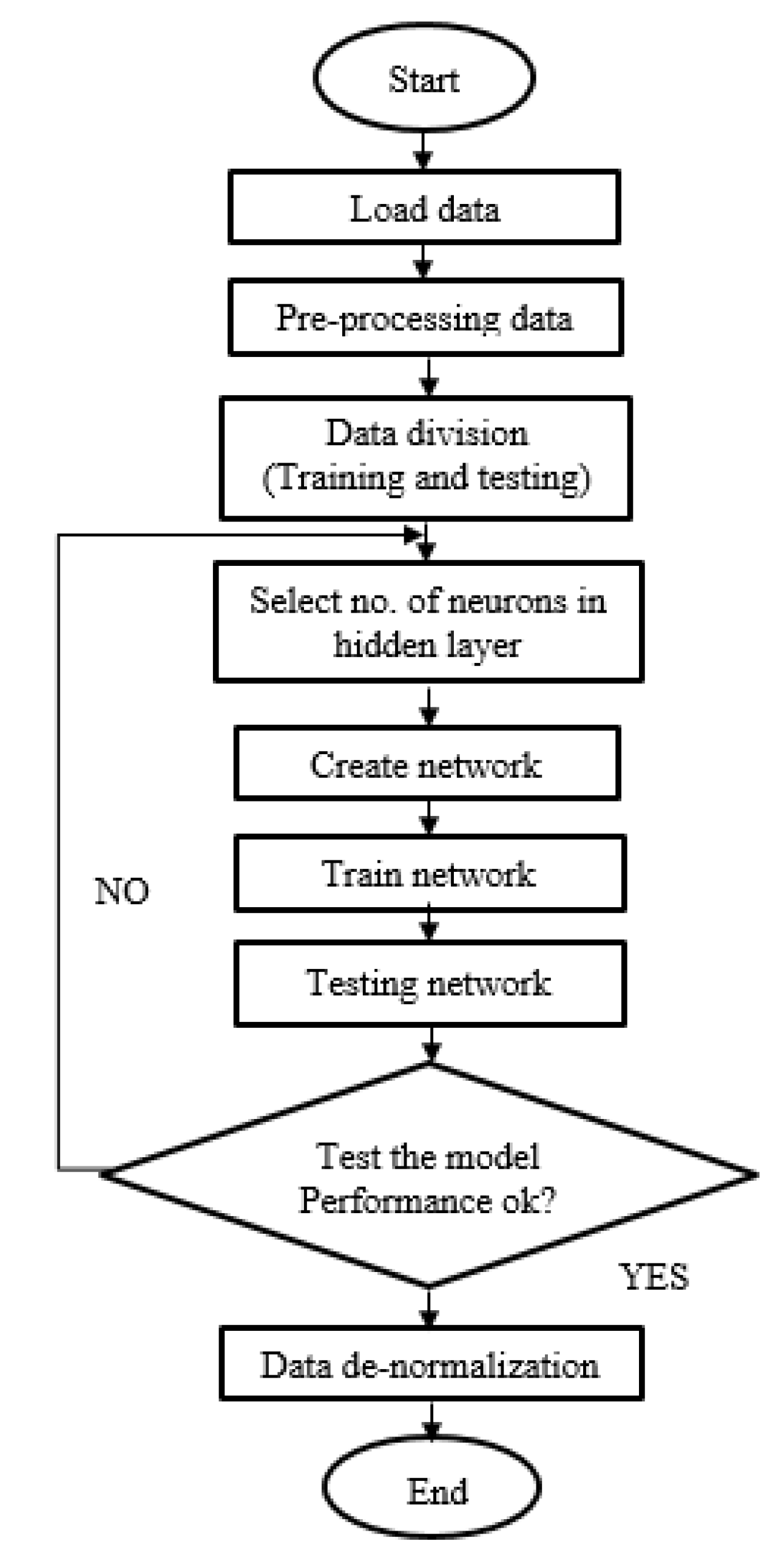
The SMBR filtration data set (4000 data samples) was utilized to develop the NARXNN models. The measured data were normalized so that the dataset was scaled in the range of (0, 1). The data were divided, as in the previous methods, into 60% for the training and 40% used for testing of the model. The determination of the structure for the NARXNN was crucial and required more effort to accomplish. The NARXNN structure consisted of three layers; the input layer, the hidden layer, and the output layer. Appropriate selection of the number of neurons in the hidden layer is very important for effective learning and performance. In this work, the NARXNN structure was varied from 1 to 10 hidden neurons and the performance was measured using MSE criteria. For each number of hidden neurons, the training was repeated eight times to determine the best, average, and worst performances. Before training, the process weights were initialized to small random numbers. The weights were adjusted till error got minimized for all training sets. In this work, the simulation result showed that the MSE for six hidden layer neurons with seven weights for flux output, and five hidden layer neuron with 11 weights for TMP output, gave the best performance.

The tan-sigmoid transfer function was employed for the hidden layer and linear weights for the output layer. They are widely used when modelling with nonlinear autoregressive exogenous neural network neural network. After selecting the learning algorithm, the number of training epochs was chosen in order to train the model. The backpropagation was utilized to train the network for 1000 training epochs as the set stooping criteria. After the training stage stopped, the NARXNN model was provided with the testing data. The prediction ability was measured based on the performance criteria using MSE, MAD, and R². The steps of developing the NARXNN are described are shown in Figure 8.

After realizing the desired model, the performance could also be evaluated using criteria presented in the following subsection. The training specifications for both forward and inverse model are presented in

Table 1. Activation function.

Parameter	Specification
Network Architecture	FFNN	RBFNN	NARXNN
Training algorithm	Levenberg Marquad
Activation function	Tan-sigmoid	Gaussian	Tan-sigmoid
Output activation	Pureline
Number of layers	3
Number of neuron hidden layer	Flux-5 TMP-7	Flux-3 TMP-3	Flux-6 TMP-5
Number of weights	Flux-10 TMP-14	Flux-10:5 TMP-8:3	Flux-7 TMP-11
Input	Permeate pump voltage
Outputs	Permeate flux and TMP
Training data	60%
Testing data	40%
Performance index	MSE, MAD, R2

. The training process involved iteratively comparing the input and target data and minimizing the error through weight adjustment until the error criteria set reduced to minimum nearest level.

2.5. Implementation of Neural Network Internal Model Control

This section presents the Neural Network Internal Model Control (IMC) methodology and its implementation to the Membrane Bioreactor System. For the IMC control architecture, it is crucial to have good estimation of model since the controller is designed based on the inverse of the model. Using the neural network, the training of the inverse model is similar to the training of the forward model. The training may vary based on the variables used as inputs and outputs of the model. The best hidden neuron structures from the network architecture for all ANN modelling methods were used to train the acquired set of 2400 data. The proper structure of the ANN model inverse model was needed. The inverse model of the SMBR filtration process built-up from FFNN, RBFNN and NARXNN which were trained by considering Flux and TMP as input data and voltage as an output data as shown in Figure 9. In this work, the backpropagation for feedforward neural network (FFNN) was used for calculating the gradients. Meanwhile, the Levenberg–Marquardt (LM) was the optimization algorithm used for training the neural network using the gradients computed with backpropagation.

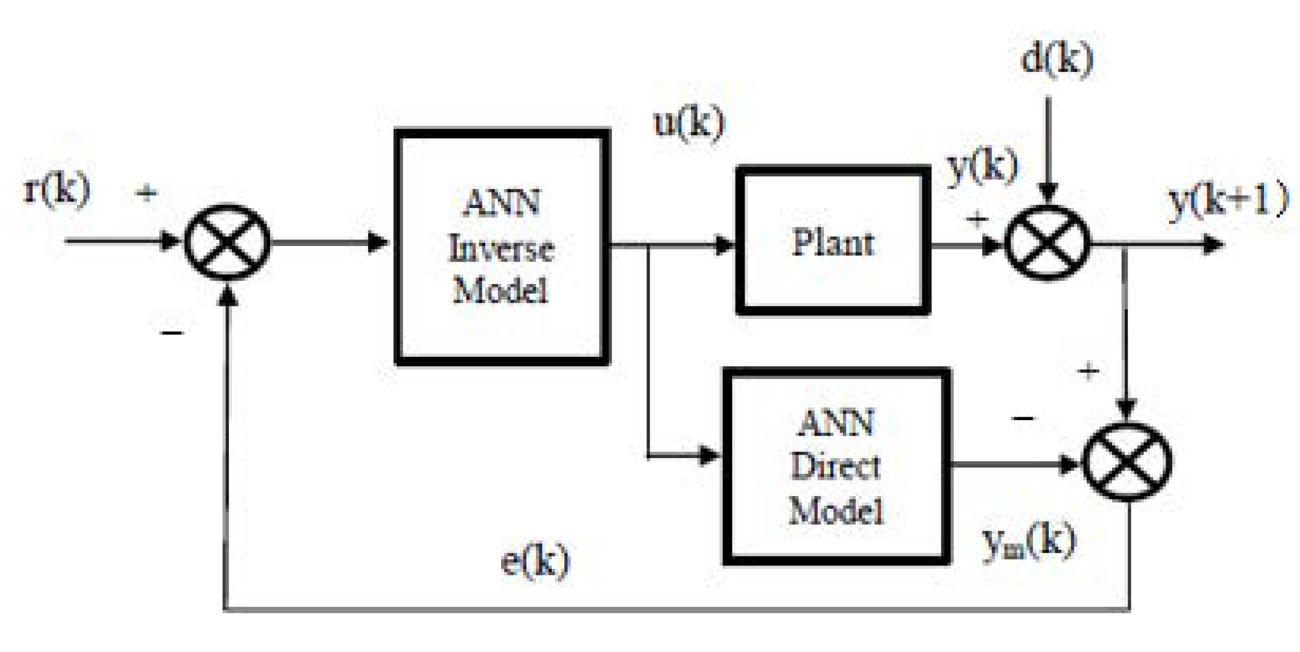
This Neural Network Internal Model Control (NNIMC) was developed to control the permeate flux as to prevent flux decline in the membrane filtration cycle due to the fouling problem. The ability of this controller to predict the plant behavior under any circumstances such as disturbance and set point change, among others, makes the controller worth implementing to control the SMBR filtration process. The NNIMC is a controller that is able to produce accurate results under nonlinear behaviour of the process plant. The disturbance rejection performance was tested through a step disturbance into the closed loop system. The Conventional IMC (C-IMC) was first developed using the best performance of modelling which was RBFNN. The block diagram of the C-IMC is shown in Figure 10. The neural network inverse model was obtained by inverting the neural network model describing the plant dynamic (using Newton’s method by solving numerically the control action from the formulation of the network forward model) or directly by using trained inverse model neural network controller. In this work, direct trained neural network was utilized to design the neural network controller.

Filter Design

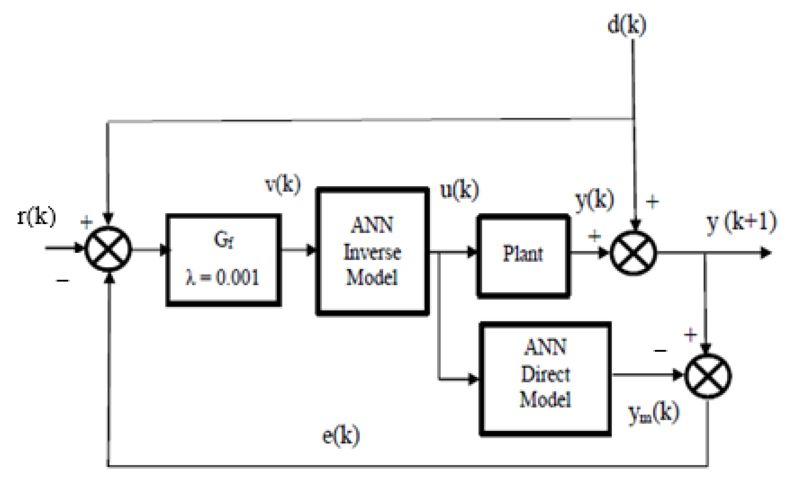
To improve robustness, the effects of mismatch between the process, and process model should be minimized. Since the differences between process and the process model usually occur at the systems high frequency response end, a low-pass filter G_f(s) is added to attenuate this effect [24]. Thus, IMC is designed using the inverse of the process model in series with a low-pass filter as shown in Figure 11. A low-pass filter was used in to filter high frequency signal components and adjusting the controller sensitivity. The filter transfer function used in this work is:

$$G_f\left(s\right)=\frac{1}{{\left(\lambda s+1\right)}^n}$$

(6)

where n is the order of the filter and λ is the filter time constant. The order of the filter was chosen so that similar to the order of the plant to ensure that the process is proper to prevent excessive differential control action. Hence, the second order filter was used. The filter time constant is an adjustable parameter which determines the speed of response. The filter parameter in the design can be chosen as a rule of thumb; hence the filter parameter values are often dictated by modeling errors, as already stated that in the design, it remains only a tunable parameter. Filter time constant shall be selected so as to obtain good closed-loop performance and disturbance rejection. The higher the value of λ, the higher the robustness of the control system. Increasing λ increased the closed loop time constant and slows the speed of the response, decreasing λ does the opposite. Usually the choice of the filter parameter depends on the allowable disturbance and noise amplification by the controller and on modeling errors. Filter time constant λ avoids the excessive noise amplification and accommodate the modeling errors. In this work, the range of the tuning parameter was varied from 0.0001 to 0.01. The best IMC filter time constant for the system was 0.001 which gave good performance both for set point tracking and disturbance rejection.

The additional filter was designed in order to improve the performance for set point and disturbance rejection. The control configuration modification consisted of a forward model, inverse model, plant, filter, and disturbance. The inverse model was obtained by a direct trained neural network using FFNN, RBFNN and NARXNN models. The inverse model acted as a controller in the system. In this work, the NNIMC with the additional filter in the system was analyzed and tested to improve the performance of system. To control fouling in membrane bioreactor filtration system, the second-order filter was used in the control scheme with the tuning parameter as 0.001. This modification had the effect of increasing system robustness in terms of disturbance rejection and hence the controller maintained its stability. To observe the effectiveness of filtering action in IMC, the performance comparison between C-IMC and the modified IMC neural network models (FFNN IMC, RBFNN IMC and NARXNN IMC) was performed.

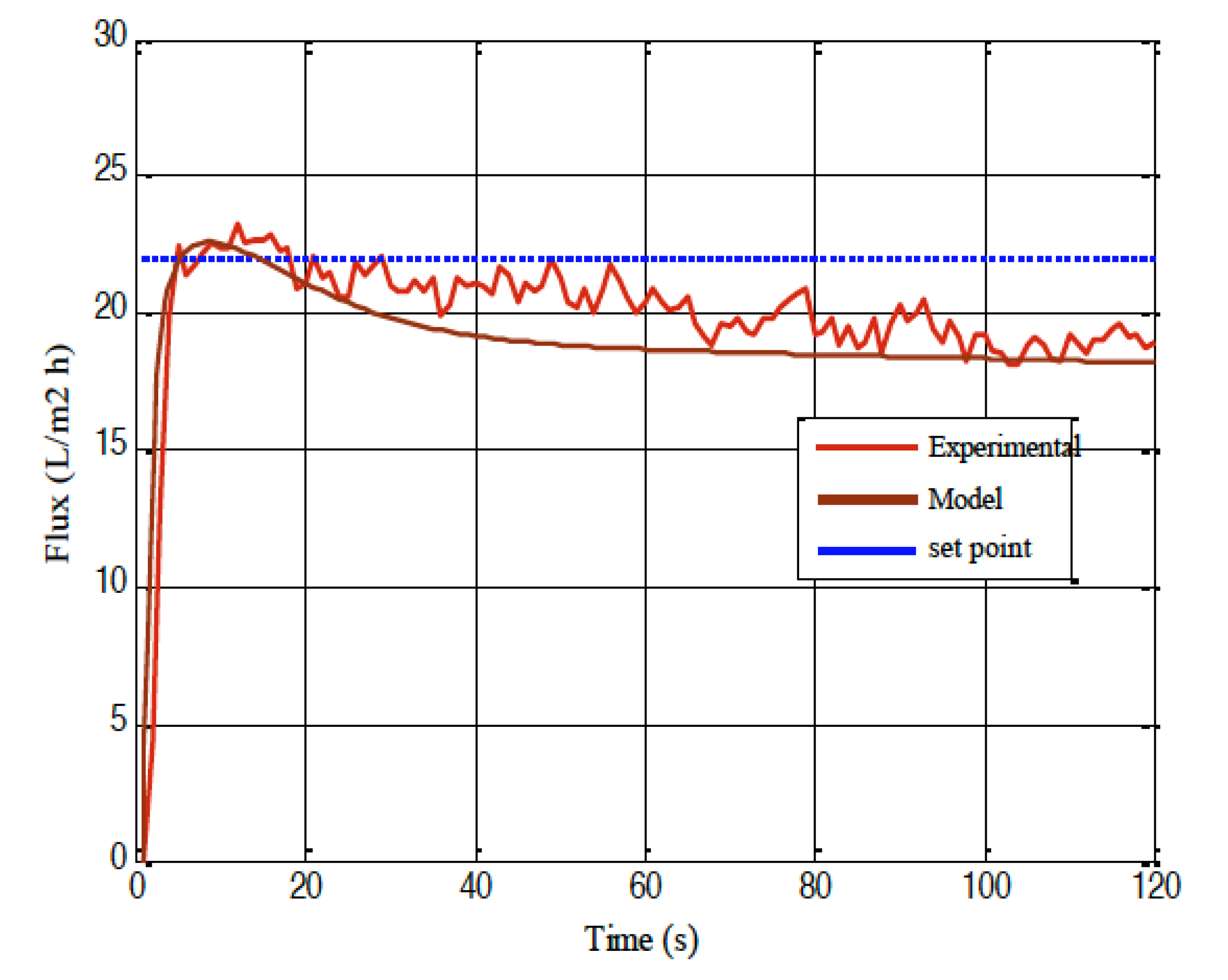
The selection of the IMC filter was based on preliminary dynamic information about open-loop process time constant. Figure 12 shows the open loop response of both the simulation model as well as the real system. In addition to seeing that the desired value for the flux was not achieved as it went descending, the open-loop time constant was approximately 1 s. Therefore, at first, values for the IMC time constant were set a little bit less than half of the open-loop time constant (0.25–0.5 s), but the flux response was too fast. A smaller filter time constant allowed for a smoother response and a more stable system. This is what motivated the search of the IMC filter time constant as lower than one order of magnitude than this initial value 0.0001 to 0.01. The final proposal was 0.001. This may seem a rather small value, however, as that one was showing better performance therefore was taken as the final value for the IMC filter, even the variability in the manipulated variable would not be large (limited).

3. Results and Discussion

This section presents the modelling and controller simulation results for the SMBR system. The dynamic behavior of the SMBR is identified or modelled before the controller design. The modelling part is the most important aspect in designing the control system for the SMBR. For modelling, the date set was divided into training (60%) and testing (40%). The permeate pump voltage was an input parameter and the outputs were the permeate flux and TMP. Three criteria were used to assess the performance of the models; MSE, MAD and R². Meanwhile, the controller performance was evaluated using rise time, settling time, and overshoot. The precision of the controller was measured using IAE, ISE, and ITAE.

3.1. Training and Testing of SMBR Filtration System

The output results of training and testing are plotted as shown in Figure 13 and Figure 14, respectively. Three different ANN model structures that were FFNN, RBFNN, and NARXNN were developed for flux and TMP outputs of the MBR filtration system. For the training results of flux and TMP, the RBFNN provided the highest accuracy, followed by NARXNN and FFNN algorithms. As can be seen in

Table 2. Performance evaluation for training results.

Flux Models	R2	MSE	MAD
FFNN	90.15	0.0057	0.0446
RBFNN	90.55	0.0055	0.0440
NARXNN	90.39	0.0056	0.0444
TMP Models	R2	MSE	MAD
FFNN	88.43	0.0061	0.0543
RBFNN	91.29	0.0050	0.0340
NARXNN	90.34	0.0059	0.0476

, The RBFNN showed an average of 90% for R² performance, both for flux and TMP models which are very good. The MSE for FFNN, RBFNN, and NARXNN was respectively 0.0057, 0.0050, and 0.0056. The MAD values are also depicted as shown in Table 2, with the lowest value contributed from the RBFNN for both flux and TMP. The RBFNN was shown to provide several advantages that made its implementation easier, its structure was simple, the convergence speed was fast when dealing with nonlinear function approximations. As per the fouling prediction, the better the signal prediction performed by the ANN, the better the capabilities to prevent undesired operation of the system. There were only three hidden neurons required by the RBFNN compared with FFNN and NARXNN which needed five and six hidden neurons, respectively. Therefore, even with no large differences, the RBFNN outperformed the other techniques.

For the testing results shown in

Table 3. Performance evaluation for testing results.

Flux Models	R2	MSE	MAD
FFNN	90.22	0.0063	0.0446
RBFNN	92.45	0.0050	0.0343
NARX NN	92.33	0.0052	0.0365
TMP Models	R2	MSE	MAD
FFNN	88.67	0.0061	0.0564
RBFNN	91.11	0.0051	0.0230
NARXNN	91.32	0.0053	0.0233

, the trend of performance is almost the same as given by the training results. For both flux and TMP, the RBFNN shows superior performance compared to the FFNN and NARXNN methods with respect to R², MSE, and MAD criteria.

For the case at hand, from the experiment work, an optimum air bubble (generated by a permeate pump voltage) is required to ensure the plant is operated at the correct setting of the plant operation. The critical flux tests and optimal relaxation test have been conducted as preliminary experiments to avoid pressure jump to happen during filtration process. The fouling development is closely related to the rapid increment of TMP, which caused the permeate flux to decline (see Figure 4). From the experiment conducted, the maximum permeate voltage is, when the TMP reached the maximum allowable point of the filtration process of SMBR. In this situation, the fouling is visible, and it can be observed from the declination of flux (see Figure 4). The maximum allowable voltage is 4 volt, and at this point, TMP reached almost 600 mbar which indicates rapid fouling development. The flux was around 35.2 L/m²h.

3.2. Step Response Performance Evaluation

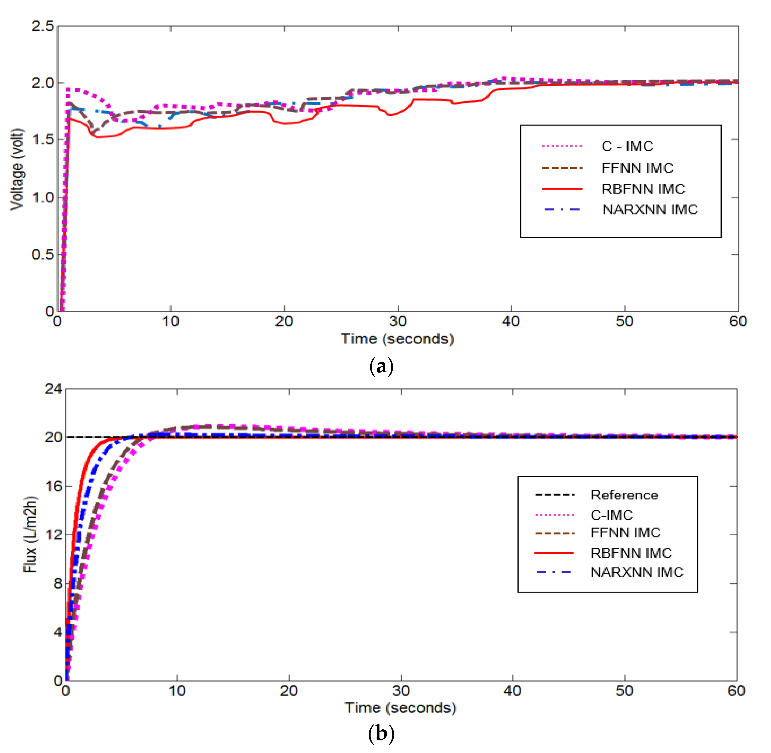
The step response evaluation was performed into the modified IMC neural network controllers and compared with the conventional IMC (C-IMC) both for setpoint and disturbance rejection performances. The setpoints for input–output response performance are presented in Figure 15a–c for all controllers. The operational setpoint for the permeate flux was given at 20 L/m²h. The numerical results are tabulated in

Table 4. Step response performance evaluations.

Controller/Criteria	Tr (s)	Ts (s)	OS (%)	IAE	ISE	ITAE
C-IMC	5.86	27.51	10.45	0.1178	0.2913	0.4245
FFNN IMC	4.53	25.77	6.73	0.0785	0.0083	0.0906
RBFNN IMC	1.51	3.75	2.44	0.0422	0.0024	0.0599
NARXNN IMC	2.04	4.52	3.98	0.0631	0.0054	0.0675

. It may be observed from Table 4 that the modified IMC neural network control showed good transient response and error performances for all criteria. The FFNN IMC and C-IMC depicted almost similar performance which settled at 25.77 s and 27.51 s, respectively. For overshoot criteria, the RBFNN IMC showed good results with only 2.44% and for NARXNN IMC it was 3.98%. The overshoot of the FFNN IMC was 6.73%, while high overshoot was produced by C-IMC with 10.45%. The TMP effect of the controller response indicated a minimal difference between each other. It could only be notified at the beginning of the controller response. From the overall result of the step response performances given in Table 4, the RBFNN IMC controller outperformed the C-IMC as well as the FFNN IMC and NARXNN IMC controllers.

3.3. Disturbance Rejection Analysis

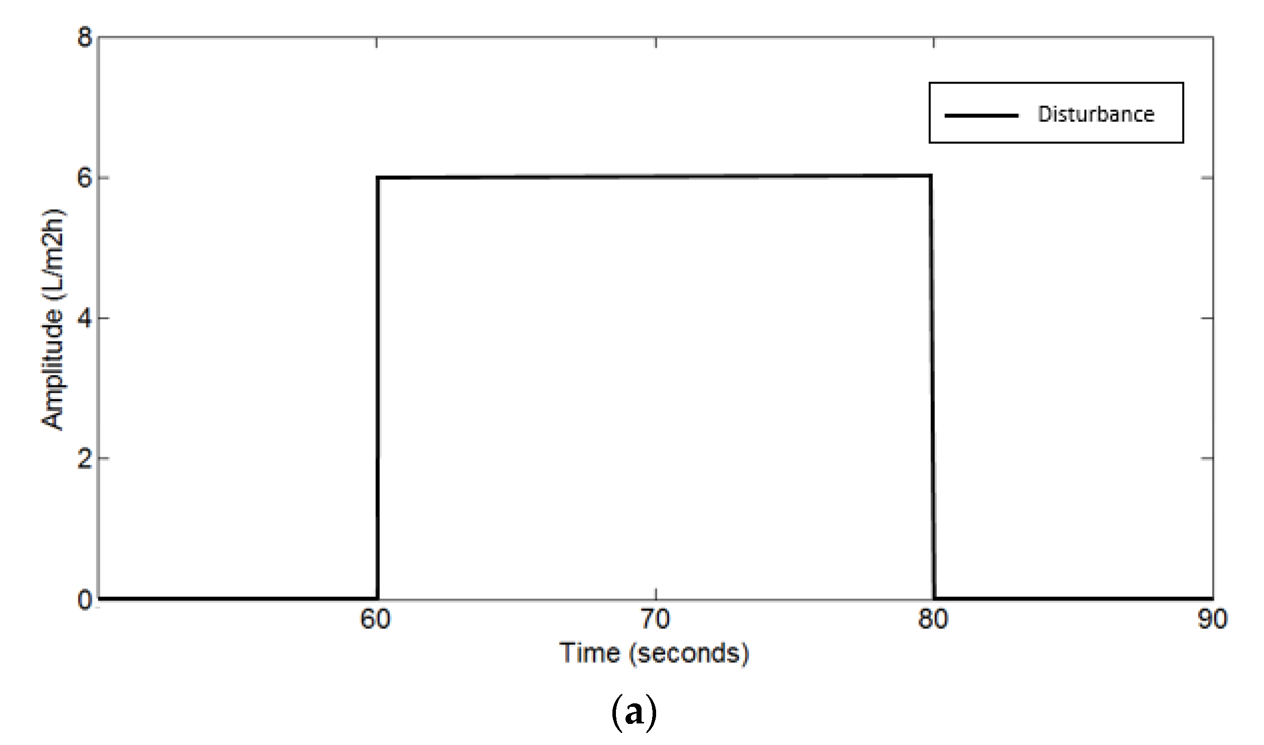
The purpose of disturbance rejection analysis is to show the robustness of the controllers despite disturbances. The disturbance was injected for an interval of 20 s into the system. The performance of the IMC controllers was evaluated and compared.

The disturbances tests were varied to investigate the robustness of the proposed controller in dealing with different amplitude of step disturbance. In this work, the output flux was increased to 2 L/m²h (10% magnitude), to 6 L/m²h (30% magnitude) and to 10 L/m²h (50% magnitude). An increased of amplitude disturbance given to the system increased the peak value.

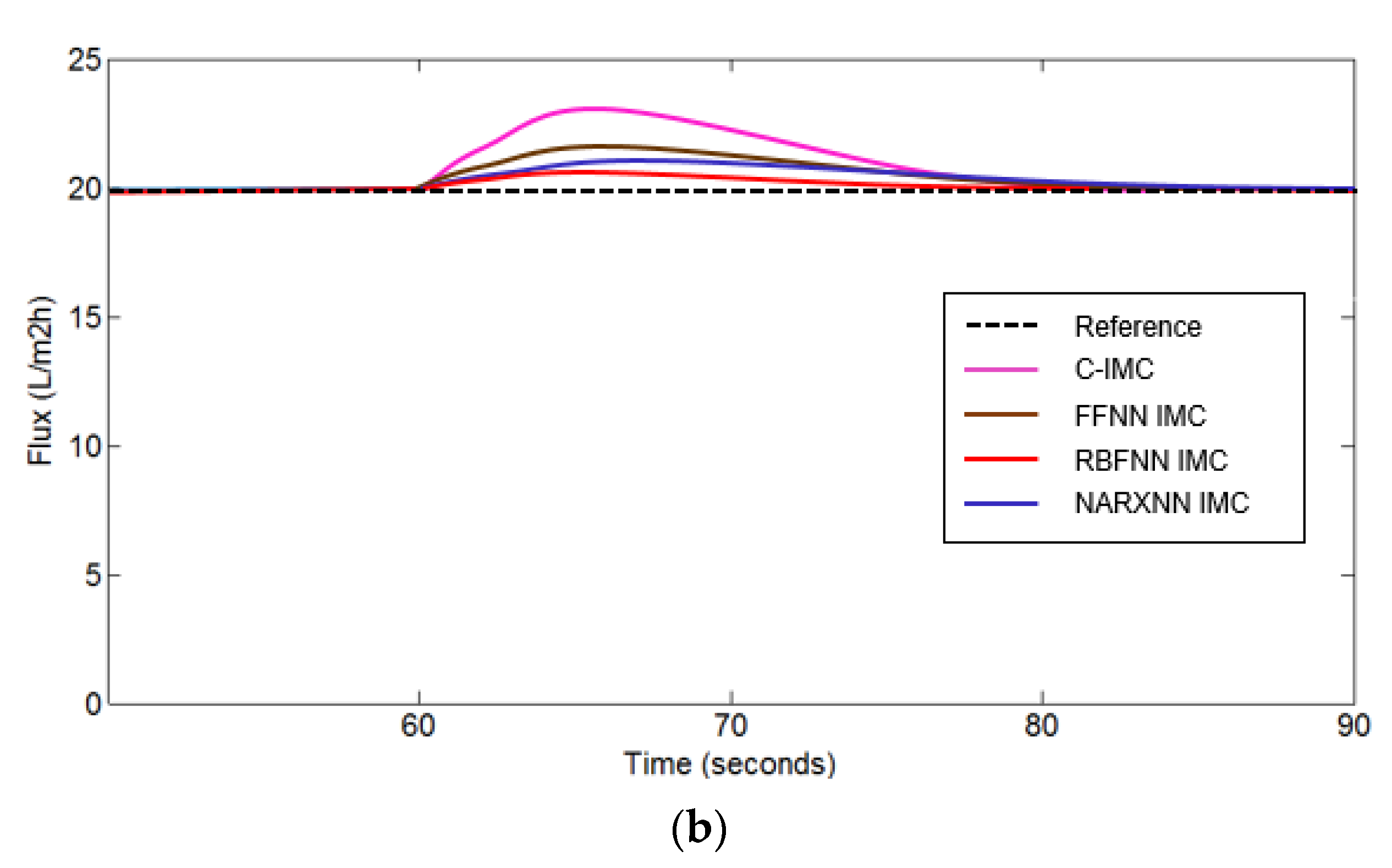
The output flux with 30% magnitude of step disturbances which resulted in 6 L/m²h was introduced at the interval time of 60 to 80 s and the performance of the system was observed as shown in Figure 16. As can be observed from Figure 16, the RBFNN IMC exhibited the best capability in rejecting the disturbance with a small overshoot (peak value) as compared with the other controllers. This was also the situation with the other tested disturbances.

The best controller for rejecting disturbance was given by the RBFNN IMC followed by NARXNN IMC and FFNN IMC. As expected, higher peak value was given by the conventional IMC for all disturbance tests and this may be due to the mismatch model conditions. This clearly demonstrated that the RBFNN IMC was effective and robust in rejecting disturbances.

3.4. Set Point Change

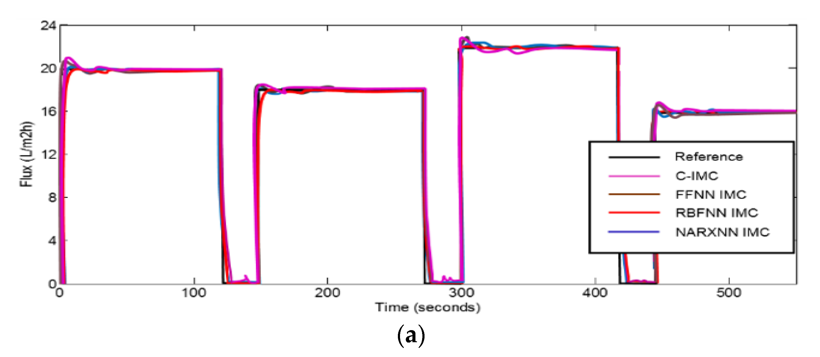
To ensure the robustness of the proposed controller, a setpoint change test was also performed to demonstrate the tracking setpoint at a different cycle. The setpoint was changed in four cycles as shown in Figure 17a–c and the performance of all controllers is presented. The setpoint of permeate flux was set at 20 and then it decreased to 18 followed by 22 and 16 respectively as shown in Figure 16a. From the operation point of view, it operated in four cycles of permeate with a period of 120 s for each cycle, while 30 s relaxation was set before change to a new set point.

The results indicated all controllers were able to track successfully the permeate flux setpoint changes. The RBFNN IMC showed good tracking performance with a small overshoot that appeared in all set points tested. The RBFNN IMC also showed little fluctuation in permeate flux control at all set points. The C-IMC exhibited slightly high overshoot with some oscillation, while the other two controllers were satisfactory.

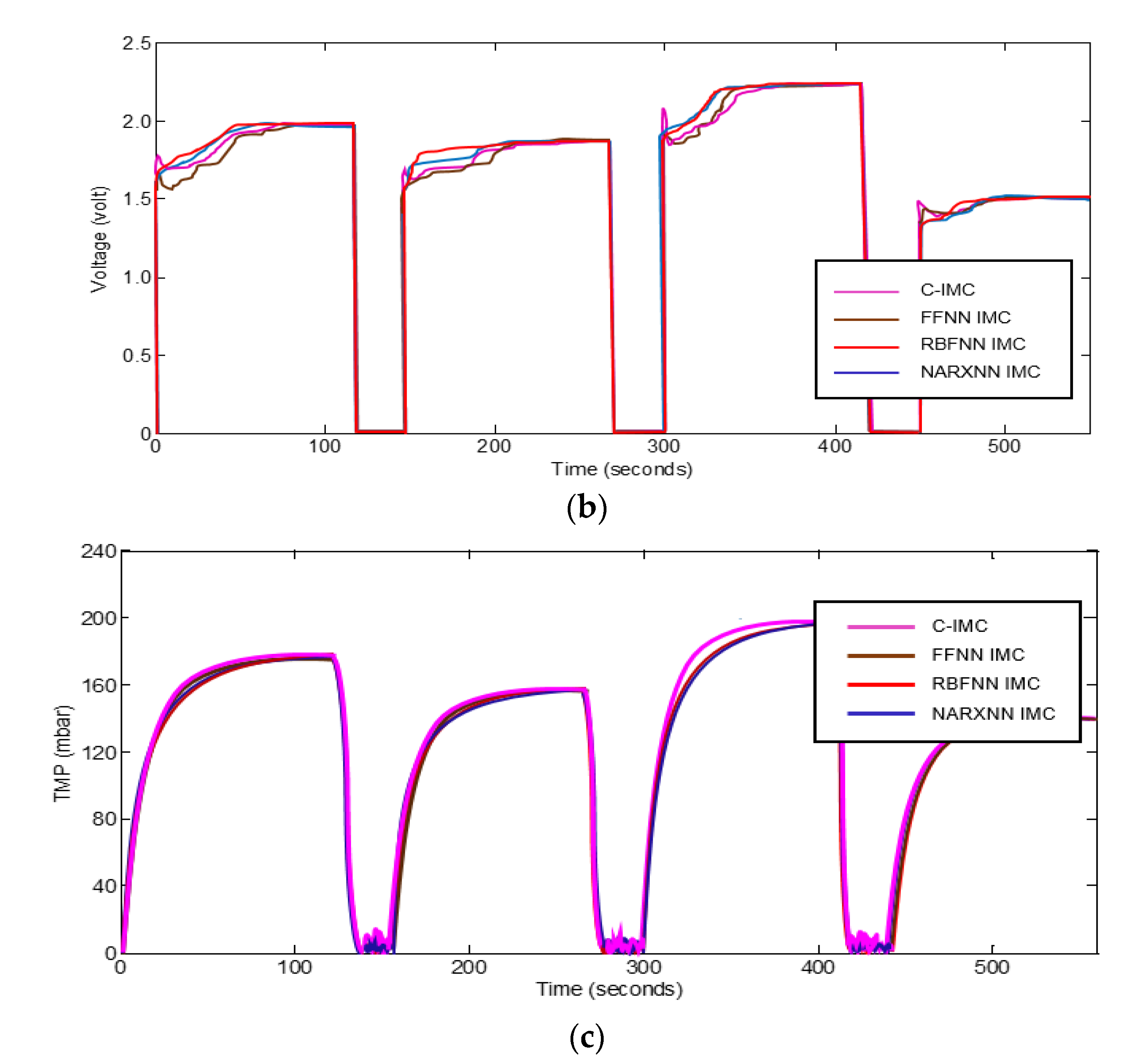
The behavior of voltage from the controllers towards the set-point tracking performance is illustrated in Figure 17b. It can be seen that all controllers exhibited similar responses, which fluctuated at the beginning of the simulation time and became more stable when the flux maintained at the set point. The C-IMC showed an excessive response of voltage at every setpoint changes test as shown in Figure 17b. The TMP profile is given in Figure 17c. Almost similar performance of the controllers is depicted. There was a slightly small deviation identified from the C-IMC controller when the TMP response was reached around 200 mbar. It is because of the high overshoot of the controller at the beginning of the cycle. Overall, the TMP profiles for each of the controllers reached the same TMP level in due course.

4. Conclusions

A new scheme for permeate flux control in SMBR by using an ANN-based IMC (or NNIMC) control structure has been investigated. The conducted work involved experimental work of SMBR system to obtain real data for the aeration fouling control system. The operating point of flux output is set to 20 L/m²h, whereby TMP is monitored so that it is operated around 200 mbar, with the permeate voltage of 2 volt. An aeration air flow is set between 6 to 8 liters per minute (LPM) to maintain high intensity of bubble flow and removing the fouling layer. The maximum allowable voltage is 4 volt, and at this point, TMP reaches almost 600 mbar which indicates rapid fouling development. The flux at this point is around 35.2 L/m²h (critical flux). The main observation that was highlighted during the experiment is, changes of the permeate pump voltage setting have an effect on permeate flux and TMP measurements

Good adaptation for RBFNN and NARXNN is achieved, both for training and testing runs which exceeded 90%. The network predictability can be improved with the increased training data set. In this work, about 60% of experimental data was used in training data set which capable to provide good learning process. The RBFNN specifically showed the highest accuracy and more reliable prediction, followed by the NARXNN and FFNN models. The RBFNN has shown to provide several advantages that makes easier its implementation, its structure is simple, the needed number of internal neurons is smaller and convergence speed is faster. As per the fouling prediction, as better the signal prediction performed by the ANN better the capabilities to prevent undesired operation of the system.

The ANN models were used for neural network internal model control design for set point tracking and disturbance rejection performances. It can be observed that RBFNN IMC and NARXNN IMC provide better performance with respect to IAE, ISE, ITAE, and overshoot for tracking and disturbance rejection performances. In addition, the effect of disturbances on flux output have been studied in a variety of magnitude steps. The RBFNN IMC performed well for all disturbance rejections (10%, 30%, 50%) compared to other IMC controllers. The RBFNN resulting control system, showed improved time response performance metrics over the other options. Whereas performance of the usual time response metrics. Settling time, for example, in NARXNN is around 80% of the one achieved by the RBFNN while not getting the 15% for FFNN. The situation is similar with respect to aggregated indexes. The IAE for RBFFN is at 67% of the one achieved by RBFFN, whereas FFNN stays at the 30% of the RBFFN achieved performance.

It can be concluded that better prediction performance can be obtained from well trained and tested ANN models. Alternatively, apply the external optimization techniques like particle swarm optimization and gravitational search algorithm. Other control techniques can be implemented to further improve the MBR filtration process such as fuzzy logic control, adaptive control, and inferential control.