Distributed Model Predictive Control Applied to a Sewer System

Abstract

In this work, a Distributed Model Predictive Control (MPC) methodology with fuzzy negotiation among subsystems has been developed and applied to a simulated sewer network. The wastewater treatment plant (WWTP) receiving this wastewater has also been considered in the methodology by means of an additional objective for the problem. In order to decompose the system into interconnected local subsystems, sectorization techniques have been applied based on structural analysis. In addition, a dynamic setpoint generation method has been added to improve system performance. The results obtained with the proposed methodology are compared to those obtained with standard centralized and decentralized model predictive controllers.

1. Introduction

Currently, it is a fact that urban wastewater treatment plants (WWTPs) have a high degree of interconnection with other elements, such as sewers, conduction systems, and storage tanks, which are part of the urban water system. Urban drainage systems (UDS) generally catch and carry both urban wastewater and that which comes from rainfall to WWTPs for treatment before being discharged into the environment, constituting a combined urban drainage system. During periods of heavy rain, the wastewater resulting from the mix can overload the urban system and produce overflows that can be harmful to the environment. Until now, UDS and WWTPs in general have been considered separately to solve their control problems.

In the case of UDS, the research has essentially consisted of the development of detailed process models that facilitate the design and simulation of different control strategies. The operational objectives are basically avoiding wastewater leaks from the collection network before being treated by the treatment plants, due to overflows in the storage tanks and at the entrance of the WWTP, optimizing the degree of use of the station by maximizing the inlet flow, and reducing the economic cost of operation [1,2]. Other problems that appear are the “first flush” problems, which occur after a dry season when abundant precipitation occurs, causing a large increase in the concentration of pollutants in the network water.

Some simulation models constitute benchmarks for the control systems of the sewer, such as [3]. On the one hand, the models try to describe with great precision the processes that take place in a drainage network (hydraulic and chemical processes of degradation of discharged pollutants) and, on the other, they have to be simple enough to be the target of simulations in the long term. In the development of these models, the characteristics of the wastewater collected according to the area (urban and industrial waters with different concentrations of pollutants), the rainwater reaching the network, and the time of year are taken into account, based on a large volume of collected data. As a result, typical patterns that attempt to cover a large number of situations have been developed [4]. From these models, simpler ones can be obtained to be used in the elaboration of certain types of control algorithms.

Regarding the control systems for UDS [5], they are usually classified into off-line controllers, which apply static rules, and improved on-line controllers that apply real-time control actions [3,6,7,8].

Table 1. Some features of real-time control systems.

Type	Based on	Pros	Cons
MPC	Optimization, needs a model	Predictive, Consider constraints and delays	Computational cost
LQR	Optimization, needs a model	Simplicity	Centralized, no constraints
RBC-FLC	Rules, heuristic	Model free	Needs expert knowledge
EA-PD	Optimization, model free	Non-linear systems	Computational cost

shows a summary of features for the real-time control systems:

In particular, simple RBC (Rule-Based Control) strategies have been applied in [9,10], offering as main disadvantage the increase of rules when the complexity of the system increases. Alternatively, FLC (Fuzzy Logic Control) based control systems that combine simple rules with an expert system and a flexible specification of the output parameters can be used [9,11,12,13,14]. An FLC is also used to reduce the volume and number of overflows in the Wilhelmshaven (Germany) UDS achieving both objectives [15]. The principles of FLC have been used to control the operation of the pumps in the collection network od the city of Taipei, achieving a more efficient drainage of rainwater, and thus preventing flooding [16]. Another type of algorithm, the LQR regulator, has been applied in [17] to flow control in a collection network in Bavaria (Germany). In this case, the control objectives were to minimize the overflows in the system by optimally using all the storage capacity of the UDS and emptying the network as soon as possible. Evolutionary Strategies (EA) mimic evolutionary principles to find optimal solutions [18]. For example, Genetic Algorithms have been applied to water quality management systems in [19] and to the optimal multiobjective control of UDS [20]. In [10], EA combined with self-adaptive algorithms has achieved an improvement in the quality of the water discharged into rivers, with reduced costs. In the control techniques based on Population Dynamics (PD), the designed controller poses a problem of resource location, and its interpretation can be related to biological evolutionary processes, without considering a system model, using game theory concepts. These strategies have been applied in [21,22], achieving a better use of network volume and avoiding overflows.

Regarding the architecture of the control systems used in UDS, one of the most common global control configurations is centralized control. However, the local control scheme may be a suitable solution if there are few actuators in the system [23]. In complex large-scale systems, it is common to have both levels of control (global and local). In this case, there can be up to three levels of control configuring a hierarchical control structure [24,25].

In the urban water systems, the interaction between the UDS and the WWTP is clear, since the outflow from the UDS is the inlet of the treatment plants. Consequently, to improve performance, the development and evaluation of control strategies for WWTPs should be addressed from a broader perspective [26]. However, there are only few works in the literature that take both systems into account in an integrated way and focus on the performance of the WWTP, using simplified models for the sewer networks [27,28]. In particular, the consideration of the integrated system allows for a bidirectional coupling of the conceptual models of the subsystems including WWTPs [29]. Regarding the applied control strategies, in [30], a heuristic-type control system based on rules that covers both situations of scarcity and abundance of water to be treated is described, also taking into account the operating costs of the entire system. Others, like [31], present strategies that combine RBC algorithms with Model Predictive Control (MPC).

MPC is a control methodology that uses a process prediction model to calculate the manipulated variables on a future horizon in order to optimize a certain cost function [32,33,34,35,36]. An MPC controller has four basic elements: a control-oriented mathematical model of the system, a cost function that expresses the control objective to be achieved, a set of system constraints, and a finite horizon optimization problem that is solved in a receding-horizon way [33]. In a hierarchical control structure, the MPC is normally used to generate optimal references for local controllers. The characteristics of MPC controllers have certain advantages for their application to UDS, particularly the ability to anticipate the system’s response to future rainfall events and the ability to consider delays and disturbances [32]. This controller has been applied to the UDS in [25], where a centralized predictive control has been developed according to a proposed model in which the state variables considered are the volumes of the network tanks, the control or manipulated variables are flow rates in the network pipes, and the measurable disturbances are the flows of rainwater. The restrictions in this case are given by the available volume of tanks and pipes, among others.

A prioritization of multi-objective cost functions is applied by means of the lexicographic technique in the control of a UDS in [37]. In [38], an MPC controller has been simulated in a part of Barcelona’s drainage network, in Spain, achieving significant reductions in floods and overflows [25,38,39,40]. Other cases in which MPC control algorithms have been studied and/or applied to UDS are [23,41,42], where both operation costs and overflows have been reduced using non-linear prediction models.

In large-scale systems, it may be advisable to divide the global process into simpler subsystems to facilitate the application of MPC algorithms [7]. In this case, prediction models and local cost functions are used, obtaining local solutions to the global control problem. If there is no exchange of information between subsystems, Decentralized Model Predictive Control is a possible solution, but a more efficient alternative is the Distributed Model Predictive Control (DMPC), where local controllers exchange information to calculate their own local solution, as in the cooperative (or Coordinated) Distributed Model Predictive Control [8,43,44,45]. Although there is a large amount of DMPC strategies applied to different processes [46,47,48], only a few deal with water management, such as the level control in tanks [49] and the coordination of drinking water supply networks [50,51,52]. To the knowledge of the authors, no applications to sewer systems have been developed.

The main contribution of this work consists in the development and application of a practical cooperative distributed model predictive control to a UDS, based on local linearized models of the system and fuzzy negotiation among subsystems [53]. Another contribution is the inclusion of the WWTP in the control strategy as an additional objective—more concretely, the optimization of the WWTP inlet flow. The benchmark described in [3] has been considered, with different disturbances, and the results have been compared with a centralized and decentralized MPC, to assess the suitability of the proposed methodology and its application to this system.

The article is structured as follows. After an introduction, the description of the system under study begins, along with the mathematical model used for the simulation and the model used by the control algorithm. In the following section, its sectorization is detailed. The article continues with the description of the centralized and distributed MPC control algorithms, showing the corresponding results in each case in two representative scenarios. The conclusions are presented at the end.

2. System Description and Evaluation Criteria

2.1. System Description

The sewer system used as a benchmark [3] (Figure 1) is made up of six rainwater and wastewater catchment areas (numbered from 1 to 6 in the figure), six wastewater storage tanks (ST1, …, ST6; one of them, ST5, is off-line), wastewater pipes, five valves and a pump for flow control, and a wastewater treatment plant (WWTP).

The objective of the sewer is to collect all the residual water and lead it to the WWTP, maintaining a supply flow with the least possible variability and as close to its nominal value as possible. This is achieved by retaining the volume collected in the tanks and releasing that volume when the collected flow is small. In addition, efforts are made to reduce as much as possible the overflows in the reservoirs in the face of extraordinarily intense precipitation, which can cause flooding and the dispersion of polluting substances potentially harmful to the environment.

The simulator has algorithms to generate different scenarios that take into account both the characteristics and the volume of urban wastewater discharged into the network and the runoff and filtrations collected by the network, produced by rainfall of different intensity and duration, in relation to the day of the week or season of the year considered.

To allow for the design and validation of the control algorithms, a simplified model has been developed. Firstly, only the hydraulic part of the benchmark has been considered. The ST5 tank has been removed, since, in the current configuration, it is not possible to exercise control over it. Thus, the ST6 tank has been renamed as tank 5 in Figure 2. The ST4 tank is considered to be equal to the rest, that is to say, the inlet valve is fixed so that all the water that enters the tank and the outlet flow is produced by opening another valve, rather than activating the pump. The simplified mathematical model of the process is made up of the following elements [54]:

-

Water catchment areas: all the water collected in the area constitutes an inlet flow to the system that is treated as a disturbance. The flows collected in each zone are denoted by q_ri, i = 1, …, 6.

-

Link elements: gravity residual water pipes in open channels, which connect the flows collected in each area with the tanks and the tanks with each other and with the treatment plant. They are modeled as first-order systems with very slow dynamics, according to their length. Their discrete mathematical model is the following:

$$q_i\left(k+1\right)=\left(1-\frac{T}{{\tau }_i}\right)q_i\left(k\right)+\left(\frac{T}{{\tau }_i}\right)q_{u,i}\left(k\right), i= 1,2,3\dots ,9,$$

(1)

where:

• q_i(k) is the output flow of the element i
• τ_i is the time constant of the element i
• T is the sampling period
• q_u,i(k) is the sum of inflows to the link element i

-

Storage tanks: reservoirs for storing wastewater. They are located in specific places throughout the network, with the possibility of overflow if a maximum level is reached. Their discrete model for the water level is:

$$\begin{gathered} h_i\left(k+1\right)=h_i\left(k\right)+\frac{T}{A_i}\left[u_{in,i}\left(k\right)-u_i\left(k\right)-q_{ov,i}\left(k\right)\right], q_{ov,i}\left(k\right)=\left\{\begin{array}{cc}0& h_i\left(k\right)\le h_{\max ,i}\\ \frac{A_i{d}_{0i}}{T}{\left[h_i\left(k\right)-h_{\max ,i}\right]}^{\frac{3}{2}}& h_i\left(k\right)>h_{\max ,i}\end{array}\right. \\ {u}_i\left(k\right)=v_i{c}_{0i}\sqrt{h_i\left(k\right)}, V_i\left(k\right)=A_i{h}_i\left(k\right), V_{\max ,i}\left(k\right)=A_i{h}_{\max ,i}\left(k\right), i= 1,2,3,4,5, \end{gathered}$$

(2)

where all parameters are referred to tank i and instant k:

• V_i(k) is the volume in use with water
• V_max,i is the maximum volume of the tank
• u_{in, i}(k) is the input flow rate
• q_{ov, i}(k) is the overflow flow rate
• d_0i is an experimental parameter related to overflow
• u_i(k) is the output flow rate
• h_i(k) is the water level
• h_max,i is the tank height
• A_i is the tank area
• v_i(k) is the opening of the tank outlet valve (control variable: v ∈ [0, 1])
• c_0i is an empirically calculated discharge coefficient for each tank that depends on the section of the outlet pipe

-

Nodes: they represent places of confluence of various residual water pipes. The resulting flow is considered the sum of the incoming flows.

In Figure 2, the complete system is shown by means of a block diagram built from the basic elements, where the catchments are represented by ovals, the link elements by rectangles, and the storage tanks by triangles. This system is analogous to the benchmark presented in Figure 1.

Then, the mathematical model corresponding to the diagram in Figure 2 was obtained. The states considered are the levels of the deposits 1, 2, 3, 4, and 5 (x₁,…,x₅) and the flow rates of the link elements 3, 7, 8, and 9, which correspond to the states (x₆,…,x₉). The output flow of link element 9 (state x₉) is in fact the inlet flow to the WWTP, provided that there is no overflow, that is, as long as it does not exceed the nominal value of the inlet flow to the WWTP. The output flows of the link elements of the catchments 1, 2, 4, 5, and 6, and the flow collected in zone 3, will be considered as measurable disturbances on the process: (d₁,…,d₆). The overflowed volume in tank 1 is collected again by the network and led to tank 4 thanks to the arrangement of the tank itself and that of the sewage network. The manipulated variables are the desired flows at the tank outputs, that in turn would constitute set points of local PID flow regulators at a lower level: (u₁,…,u₅). All states will be considered as outputs of the system, with a special interest in the input flow to the treatment plant. Hence, the states vector, the manipulated variables vector, and the disturbances vector are defined as follows in terms of the benchmark variables:

$$x=\left(h_1,h_2,h_3,h_4,h_5,q_3,q_7,q_8,q_9\right), u=\left(u_1,u_2,u_3,u_4,u_5\right), d=\left(q_1,q_2,q_4,q_5,q_6,q_{r3}\right),$$

(3)

The set of discrete differential equations of the non-linear mathematical model is:

$$\begin{gathered} x_1\left(k+1\right)=x_1\left(k\right)+\frac{T}{A_1}\left[d_1\left(k\right)-u_1\left(k\right)-q_{ov1}\left(k\right)\right] \\ {x}_2\left(k+1\right)=x_2\left(k\right)+\frac{T}{A_2}\left[d_2\left(k\right)-u_2\left(k\right)-q_{ov2}\left(k\right)\right] \\ {x}_3\left(k+1\right)=x_3\left(k\right)+\frac{T}{A_3}\left[x_6\left(k\right)-u_3\left(k\right)-q_{ov3}\left(k\right)\right] \\ {x}_4\left(k+1\right)=x_4\left(k\right)+\frac{T}{A_4}\left[d_3\left(k\right)+u_1\left(k\right)+q_{ov1}\left(k\right)+u_3\left(k\right)-u_4\left(k\right)-q_{ov4}\left(k\right)\right] \\ {x}_5\left(k+1\right)=x_5\left(k\right)+\frac{T}{A_5}\left[x_8\left(k\right)-u_5\left(k\right)-q_{ov5}\left(k\right)\right] \\ \mathrm{where} q_{ov,i}\left(k\right)=\left\{\begin{array}{cc}0& x_i\left(k\right)\le h_{\max i}\\ \frac{A_i{d}_{0i}}{T}{\left[x_i\left(k\right)-h_{\max i}\right]}^{\frac{3}{2}}& x_i\left(k\right)>h_{\max i}\end{array}\right., i= 1,\dots ,5 \\ {x}_6\left(k+1\right)=\left(1-\frac{T}{{\tau }_3}\right)x_6\left(k\right)+\left(\frac{T}{{\tau }_3}\right)\left[d_6\left(k\right)+u_2\left(k\right)\right] \\ {x}_7\left(k+1\right)=\left(1-\frac{T}{{\tau }_7}\right)x_7\left(k\right)+\left(\frac{T}{{\tau }_7}\right)u_4\left(k\right) \\ {x}_8\left(k+1\right)=\left(1-\frac{T}{{\tau }_8}\right)x_8\left(k\right)+\left(\frac{T}{{\tau }_8}\right)\left[d_4\left(k\right)+d_5\left(k\right)+x_7\left(k\right)\right] \\ {x}_9\left(k+1\right)=\left(1-\frac{T}{{\tau }_9}\right)x_9\left(k\right)+\left(\frac{T}{{\tau }_9}\right)u_5\left(k\right), \end{gathered}$$

(4)

From this model, a linear model of the system is obtained removing the overflow flow rate terms, to be used as a prediction model in the linear MPC algorithm. The state space model equations are the following:

$$\begin{gathered} x\left(k+1\right)=Ax\left(k\right)+B_{p}u\left(k\right)+B_{d}d\left(k\right)\Rightarrow x\left(k+1\right)=Ax\left(k\right)+B\left[\begin{array}{c}u\left(k\right)\\ d\left(k\right)\end{array} \right], \\ \mathrm{where}: B=[\begin{array}{cc}{B}_p& B_d\end{array}], x=\left(x_{1,}{x}_2,\dots ,x_9\right),d=\left(d_{1,}{d}_2,\dots ,d_6\right),u=\left(u_{1,}{u}_2,\dots ,u_5\right), \end{gathered}$$

(5)

And the matrices of the model are:

$$A=\left(\begin{array}{ccccccccc}1& 0& 0& 0& 0& 0& 0& 0& 0\\ 0& 1& 0& 0& 0& 0& 0& 0& 0\\ 0& 0& 1& 0& 0& \frac{T}{A_3}& 0& 0& 0\\ 0& 0& 0& 1& 0& 0& 0& 0& 0\\ 0& 0& 0& 0& 1& 0& 0& \frac{T}{A_5}& 0\\ 0& 0& 0& 0& 0& \left(1-\frac{T}{{\tau }_3}\right)& 0& 0& 0\\ 0& 0& 0& 0& 0& 0& \left(1-\frac{T}{{\tau }_7}\right)& 0& 0\\ 0& 0& 0& 0& 0& 0& \frac{T}{{\tau }_8}& \left(1-\frac{T}{{\tau }_8}\right)& 0\\ 0& 0& 0& 0& 0& 0& 0& 0& \left(1-\frac{T}{{\tau }_9}\right)\end{array}\right)B_p=\left(\begin{array}{ccccc}-\frac{T}{A_1}& 0& 0& 0& 0\\ 0& -\frac{T}{A_2}& 0& 0& 0\\ 0& 0& -\frac{T}{A_3}& 0& 0\\ \frac{T}{A_4}& 0& \frac{T}{A_4}& -\frac{T}{A_4}& 0\\ 0& 0& 0& 0& -\frac{T}{A_5}\\ 0& \frac{T}{{\tau }_3}& 0& 0& 0\\ 0& 0& 0& \frac{T}{{\tau }_7}& 0\\ 0& 0& 0& 0& 0\\ 0& 0& 0& 0& \frac{T}{{\tau }_9}\end{array}\right),$$

(6)

$$B_d=\left(\begin{array}{cccccc}\frac{T}{A_1}& 0& 0& 0& 0& 0\\ 0& \frac{T}{A_2}& 0& 0& 0& 0\\ 0& 0& 0& 0& 0& 0\\ 0& 0& \frac{T}{A_4}& 0& 0& 0\\ 0& 0& 0& 0& 0& 0\\ 0& 0& 0& 0& 0& \frac{T}{{\tau }_3}\\ 0& 0& 0& 0& 0& 0\\ 0& 0& 0& \frac{T}{{\tau }_8}& \frac{T}{{\tau }_8}& 0\\ 0& 0& 0& 0& 0& 0\end{array}\right)C=I_9,$$

2.2. Evaluation Criteria

The following evaluation criteria are used to analyze the behavior of the system and the effects of the applied control strategies. The evaluation considers different points of overflow in the sewer network and at the entrance of the treatment plant [3]. Some of them only consider hydraulic magnitudes, while others also consider variables related to water quality. Among the indices corresponding to the first group, the most used are shown below, where the subscript i represents the specific point in the system:

• Number of overflows (N_ov,i): this criterion represents the total number of overflow events that have taken place at a certain point in the network. Two overflow events that are less than an hour apart are considered a single event.
• Duration of overflow (T_ov,i): this criterion represents the cumulative sum of the duration of all overflow events at a certain point in the system at simulation time T_sim (d). If each event j lasts t_j days and n events take place, the overflow duration is given by the expression:

  $$T_{ov,i}={\displaystyle \sum _{j=1}^n{t}_j},$$

  (7)
• Overflow volume (V_ov,i) (m³): it is the total volume of wastewater discharged into the receiving waters receivers from a certain overflow point i. Considering simulation time T_sim and overflow q_ov,i(t):

  $$V_{ov,i}={\displaystyle \underset{0}{\overset{T_{sim}}{\int }}{q}_{ov,i}\left(t\right)dt},$$

  (8)

  and the total overflow volume is:

  $$V_{ov}={\displaystyle \sum _{i=1}^n{V}_{ov,i}},$$

  (9)
• Degree of usage of WWTP (G_u,i) (%): the ratio of the average flow rate in the simulation time and the nominal flow rate $q_{WWTPnom,i}$ of the plant i, in percent:

  $$G_{u,i}=\frac{100}{q_{WWTPnom,i}\cdot T_{sim}}{\displaystyle \underset{0}{\overset{T_{sim}}{\int }}{q}_{WWTP,i}\left(t\right)dt},$$

  (10)
• Smoothness in the application of control signals (flows) on the system (m⁶/d²): it can be measured from variations in control actions u(k) between the instant k and k − 1 in the simulation time, by means of the following expression:

  $$S={\displaystyle \sum _{k=1}^N{\left(u\left(k\right)-u\left(k-1\right)\right)}^T}\left(u\left(k\right)-u\left(k-1\right)\right), N=\frac{T_{sim}}{T},$$

  (11)

3. System Sectorization

Applying control techniques to large-scale systems usually involves dividing the global system into simpler subsystems. To this end, a structural analysis of the system has been carried out to determine the best way to sectorize the system, so that the subsystems obtained have a minimum degree of coupling and are controllable [55]. With this end, the reachability from the entrance of the system has been checked, and the direct graph of the system has been obtained.

Definition: A system S with a direct graph D = (U∪X∪Y, E) is input-reachable if X⊆ℜⁿ is a reachable set of U⊆ℜ^m, that is, for each node x∈X there is at least one node u∈U with a direct path to it.

Definition: A system S with a direct graph D = (U∪X∪Y, E) is output-reachable if X⊆ℜⁿ is an antecedent set of Y⊆ℜ^r, that is, for each node x∈X there is at least one node y∈Y with a direct path to it.

Then, a system S is reachable if it is input- and output-reachable. The study of the reachability of the system allows us to determine the possibilities of sectoring while maintaining the reachability of the subsystems obtained. It begins with obtaining the interconnection matrix E, which is defined from the matrices that determine the dynamic model of the system, A, B_p, and C, as:

$$\begin{gathered} E=\left(\begin{array}{ccc}\overline{A}& {\overline{B}}_p& 0\\ 0& 0& 0\\ \overline{C}& 0& 0\end{array}\right),\mathrm{where} \overline{A}, {\overline{B}}_p, \mathrm{and} \overline{C}\mathrm{are} \mathrm{given} \mathrm{by}: \\ {\overline{a}}_{ij}=\left\{\begin{array}{l}1,a_{ij}\ne 0\hfill \\ 0,a_{ij}=0\hfill \end{array}\right.,{\overline{b}}_{ij}=\left\{\begin{array}{l}1,b_{ij}\ne 0\hfill \\ 0,b_{ij}=0\hfill \end{array}\right.\mathrm{and} {\overline{c}}_{ij}=\left\{\begin{array}{l}1,c_{ij}\ne 0\hfill \\ 0,c_{ij}=0\hfill \end{array}\right., \end{gathered}$$

(12)

Reachability matrix R can be computed as $R=E\vee E^2\vee \dots \vee E^s$, with $s=\dim E$, and it has the following form:

$$R=\left(\begin{array}{ccc}F& G& 0\\ 0& 0& 0\\ H& \theta & 0\end{array}\right),$$

(13)

where F, G, H, and θ are binary matrices whose dimensions are consistent with E.

The system will be input- and output-reachable if and only if the binary matrix θ has neither zero rows nor zero columns [55].

For the sewer system considered here, the following matrix θ has been obtained, resulting in a system that is reachable from the input and the output:

$$\mathrm{\theta }=\left(\begin{array}{ccccc}1& 0& 0& 0& 0\\ 0& 1& 0& 0& 0\\ 0& 1& 1& 0& 0\\ 1& 0& 1& 1& 0\\ 0& 0& 0& 1& 1\\ 0& 1& 0& 0& 0\\ 0& 0& 0& 1& 0\\ 0& 0& 0& 1& 0\\ 0& 0& 0& 0& 1\end{array}\right),$$

(14)

Moreover, obtaining the direct graph of the system (Figure 3) will allow us to know the interactions between the different variables that are involved in the process and determine the best way to divide the global system into subsystems with minimal interaction [36], maintaining the reachability of the subsystems obtained.

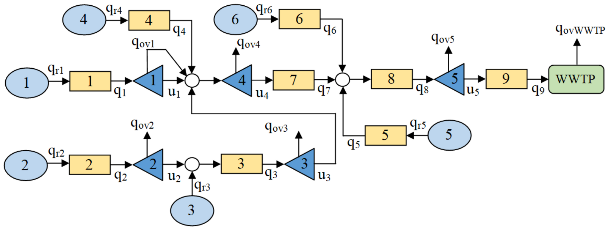
The graph shows a system coupled by the inputs. The sectoring has been carried out avoiding interactions between states of different subsystems and at the same time ensuring their reachability (Figure 4). The controllability of each subsystem can be verified. Accordingly, this work considers two subsystems, the first one englobing the tanks 1 to 4 together with link element 3, and the second one tank 5 and link elements 7, 8, and 9.

To apply the distributed MPC developed in Section 7, the state space local models of each subsystem are expressed as follows, where the coupling input u₄ is considered to belong to subsystem 1.

$$\begin{gathered} x_1\left(k+1\right)=A_1{x}_1\left(k\right)+B_{p11}{u}_1\left(k\right)+B_{p12}{u}_2\left(k\right)+B_{d11}{d}_1\left(k\right)+B_{d12}{d}_2\left(k\right), y_1\left(k\right)=C_1{x}_1\left(k\right), \mathrm{where}: \\ {x}_1=\left(x_1,x_2,x_3,x_4,x_6\right),u_1=\left(u_1,u_2,u_3,u_4\right), d_1=\left(d_1,d_2,d_3,d_6\right), \\ {x}_2\left(k+1\right)=A_2{x}_2\left(k\right)+B_{p21}{u}_1\left(k\right)+B_{p22}{u}_2\left(k\right)+B_{d21}{d}_1\left(k\right)+B_{d22}{d}_2\left(k\right), y_2\left(k\right)=C_2{x}_2\left(k\right), \mathrm{where}: \\ {x}_2=\left(x_5,x_7,x_8,x_9\right),u_2=\left(u_5\right), d_2=\left(d_4,d_5\right), \end{gathered}$$

(15)

Matrices A₁, B_p11, B_p12, A₂, B_p21, and B_p22 are formed by suitably selecting the rows and columns of A and B from the matrices (6). Note that B_p12 and B_d12 are null; B_p21 only has non-zero in the last column, and B_d21 is null, due to the plant’s configuration.

4. Control Problem

4.1. Control Objectives

The following evaluation criteria are used to analyze the behavior of the system, and the effect of the main control objective is to ensure an input flow to the WWTP as close as possible to its nominal value, making the most of its capacity, avoiding as much as possible overflows in the tanks and at the wastewater plant itself, and also minimizing operating costs. To achieve the proposed control objective, the outlet flow rates of the tanks (manipulated variables) are calculated to minimize the difference between the flow rate of the inlet to the treatment plant and its nominal value. Moreover, the volume of water at each instant is evenly distributed among all the tanks in the network, which is achieved by minimizing the difference between the water level of each tank and a dynamically calculated reference level to achieve that goal [54]. The uniform distribution of the water stored in the tanks will reduce the effects of the disturbances (collected flows at the catchment areas), minimizing the overflows. Mathematically, the control objective can be formulated by means of a cost function that includes the partial objectives previously exposed [54,56]:

$$J={\displaystyle \sum _{j=1}^M{\displaystyle \sum _{k=0}^N{w}_j{\varphi }_j\left(x\left(k\right),u\left(k\right)\right)}},$$

(16)

where N is the prediction horizon, φ_j is a partial objective, and w_j is the weight corresponding to each partial objective φ_j, with j = 1, ..., M.

In the problem considered, the following partial objectives are taken into account:

• Minimization of overflows and uniform distribution of the stored volume of water:

  $$\begin{gathered} {\varphi }_1\left(x\left(k\right)\right)={\displaystyle \sum _{i=1}^5{q}_i\left(k\right){\left(V_i\left(k\right)-v_i{V}_G\left(k\right)\right)}^2}, v_i=\frac{V_{i\max }}{{\displaystyle \sum _{j=1}^5{V}_{j\max }}}, V_G\left(k\right)={\displaystyle \sum _{j=1}^5{V}_j}\left(k\right), \\ \mathrm{with} q_i\left(k\right)=\left\{\begin{array}{cc}{f}_i& x_i\left(k\right)\le h_{\max i}\\ f_i\left(1+{\alpha }_i{\left(x_i\left(k\right)-h_{\max i}\right)}^2\right)& x_i\left(k\right)>h_{\max i}\end{array}\right., \end{gathered}$$

  (17)

  where $V_G$ is the total occupied volume in the sewer at instant k and v_i is a factor that represents the weight of the tank capacity i in the total available storage volume in the sewer. The variable weight q_i(k) allows for the overflows’ penalization, increasing its value proportionally to the corresponding overflow. Parameters f_i and α_i are used to prioritize overflows in some tanks.
• Maximum usage of the treatment plant and minimum overflow at the WWTP influent:

  $${\varphi }_2\left(x\left(k\right)\right)={\left(Q_{WWTP}\left(k\right)-Q_{WWTP\max }\right)}^2,$$

  (18)

  where Q_WWTP is the inlet flow to the WWTP at instant k and Q_WWTPmax its nominal value.
• Control efforts minimization:

  $${\varphi }_3\left(u\left(k\right)\right)={\displaystyle \sum _{i=1}^5{r}_i{\left(u_i\left(k\right)-u_{iref}\left(k\right)\right)}^2},$$

  (19)

  where u_iref are the output flows needed to keep the desired level in a tank, obtained by Bernoulli’s law. Weights r_i are tuning parameters.

4.2. Hierarchical Control System

The control system presents a hierarchical structure as shown in Figure 5 [23,25]. At the upper level, the level set point signals are generated for each tank to achieve the indicated control objectives. This will be done following the strategy of uniform distribution of the total volume occupied among all the deposits, called EFD (Equal Filling Degree) [57], which has been shown to be among the most effective dealing with overflow problems. Subsequently, the MPC controller calculates the set points to be applied to local controllers by solving a constrained optimization problem, maximizing the use of WWTP and reducing operating costs. Finally, the local controllers are in charge of the effective control of the process variables [58].

5. Centralized Predictive Control

5.1. Optimization Problem

The Centralized Predictive Control considered in this work includes a linear state space model for prediction, considering the effect of perturbations. The cost function (objective function) of the MPC is a quadratic form that takes into account both the tracking errors in the states and the deviations in the control sequence from the flow reference (therefore penalizing control efforts), assuming that the prediction and control horizons coincide and their value is N:

$$J\left(k,U\right)={\displaystyle \sum _{i=0}^{N-1}\left[{‖\widehat{x}\left(k+i\right)-x_{ref}‖}_{Q\left(k\right)}^2+{‖u\left(k+i\right)-u_{ref}‖}_R^2\right]+x^T\left(k+N\right)}Px\left(k+N\right),$$

(20)

where $x_{ref}\left(k\right)=(x_{1ref},x_{2ref},\dots ,x_{9ref})$ and $u_{ref}\left(k\right)=(u_{1ref},u_{2ref},\dots ,u_{5ref})$ are the states and inputs references, respectively, and $U(k)={\left[\begin{array}{cccc}u\left(k\right)& u\left(k+1\right)& \dots & u\left(k+N-1\right)\end{array}\right]}^T$.

The optimization problem for the centralized MPC is:

$$\begin{gathered} U_{}^{*}(k)=\underset{U\left(k+i\right)}{\arg \min J\left(k\right)}, U_{}^{*}(k)={\left[\begin{array}{cccc}{u}^{*}\left(k\right)& u^{*}\left(k+1\right)& \dots & u^{*}\left(k+N-1\right)\end{array}\right]}^T \\ \mathrm{subject} \mathrm{to}: \\ \widehat{x}\left(k+i+1\right)=A\widehat{x}\left(k+i\right)+B_{p}u\left(k+i\right)+B_{d}d\left(k+i\right), d\left(k+i\right)=d\left(k\right) \\ \widehat{x}\left(k\right)=x\left(k\right) \\ 0\le {\widehat{x}}_j\left(k+i\right)\le q_{\max j}, i=0,\dots ,N-1, j=6,\dots ,9 \\ 0\le u_j\left(k+i\right)\le u_{\max j}, i=0,\dots ,N-1, j=1,\dots ,5, \end{gathered}$$

(21)

where $q_{\max j}$ and $u_{\max j}$ are the upper bounds for flow in the linking elements and the tank outputs, respectively.

Matrices Q(k) and R and the horizon N are tuning parameters for the controller, and matrix P is a terminal penalty for MPC stability obtained by means of the Riccati equation [59]. Note that a variable diagonal matrix Q(k) has been considered to somehow prevent overflows in the tanks, excepting tank 1, because the overflow returns to the sewer. If an overflow is produced in a tank, the corresponding weight is increased to further penalize the deviation from the reference for that tank. The non-zero elements of Q(k) are q₁,…, q₅, and q₉, and are obtained by (17), where f_i and α_i are tuning parameters. The rest of the elements are zero because they correspond to state variables of link elements that are not necessary to follow any set point. Matrix R is a diagonal matrix that penalizes the variations in the flow set points with respect to their reference value, which is related to the cost of operation.

This optimization problem corresponds to a quadratic optimization problem (QP) with constraints [32]. The implemented algorithm keeps the last applied solution, so that if the optimization problem is not feasible, the last feasible solution is applied.

5.2. Set Point Calculations

To achieve optimal operation, we designed a hierarchical controller that modifies, in a higher layer, the tanks’ level set points according to the strategy of distributing the current volume of water among all the tanks in the most uniform way possible considering their capacity [57]. This is achieved by calculating for each one its reference level, based on the total capacity of the network and the capacity of that deposit at each sampling instant:

$$x_{iref}\left(k\right)=\left(\frac{V_G\left(k\right)}{A_i}\right)v_i,$$

(22)

where $x_{iref}\left(k\right)$ is the reference level for tank i at instant k. The references for the states $x_{6ref}$,$x_{7ref}$, and $x_{8ref}$ would be zero because they are outflows of link elements that are not considered. Moreover, $x_{9ref}=60.000$m³/d, which is the nominal influent flow to the WWTP.

The flow setpoints are calculated taking into account the desired level for each tank, according to expression:

$$u_{iref}\left(k\right)=c_{0i}\sqrt{x_{iref}\left(k\right)}, i=1,\dots ,5,$$

(23)

The references are updated every two sampling periods, which is sufficient considering the dynamics of the system and the disturbances.

6. Distributed Model Predictive Control (DMPC)

The DMPC algorithm considered in this work is based on [60], consisting of the minimization of local cost functions that depend on the future evolution of the inputs of each subsystem and the neighbor, using prediction models and local constraints. At each sampling period, agents get an optimal control sequence for their subsystem, keeping the neighbor control sequence constant, and then each agent solves another optimization problem that provides the control sequence for the neighbor, keeping theirs constant.

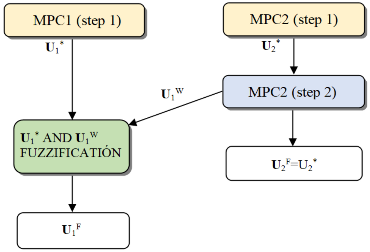
Due to the particular characteristics of this system, since there is no interaction of the inputs of subsystem 2 in subsystem 1, the procedure is simplified, and some of the optimization problems of the general method are not solved. Figure 6 gives an overview of the algorithm.

And it consists of several steps:

STEP 1: The state measurements $x_1\left(k\right)$ and $x_2\left(k\right)$ corresponding to each subsystem are obtained at instant k. Two local predictive control problems (MPC1 and MPC2) are solved, obtaining local solutions $U_1^{*}$ and $U_2^{*}$ for each subsystem:

MPC1 objective function:

$$\begin{gathered} J_1\left(k,U_1,U_2\right)={\displaystyle \sum _{i=0}^{N-1}\left[{‖{\widehat{x}}_1\left(k+i\right)-x_{1ref}\left(k\right)‖}_{Q_1\left(k\right)}^2+{‖u_1\left(k+i\right)-u_{1ref}\left(k\right)‖}_{R_1}^2\right]+x_1^T\left(k+N\right)}{P}_1{x}_1\left(k+N\right), \mathrm{where} \\ {x}_{1ref}\left(k\right)=(x_{1ref},x_{2ref},x_{3ref},x_{4ref},x_{6ref}),u_{1ref}\left(k\right)=(u_{1ref},u_{2ref},u_{3ref},u_{4ref}), \\ {U}_i(k)={\left[\begin{array}{cccc}{u}_i\left(k\right)& u_i\left(k+1\right)& \dots & u_i\left(k+N-1\right)\end{array}\right]}^T, i= 1,2, \end{gathered}$$

(24)

The optimization problem is:

$$\begin{gathered} U_1^{*}\left(k\right)=\underset{U_1\left(k+i\right)}{\arg \min J_1\left(k,U_1,U_2\right)},U_1^{*}(k)={\left[\begin{array}{cccc}{u}_1^{*}\left(k\right)& u_1^{*}\left(k+1\right)& \dots & u_1^{*}\left(k+N-1\right)\end{array}\right]}^T \\ \mathrm{subject} \mathrm{to}: \\ {\widehat{x}}_1\left(k+i+1\right)=A_1{\widehat{x}}_1\left(k+i\right)+B_{p11}{u}_1\left(k+i\right)+B_{p12}{u}_2\left(k+i\right)+B_{d11}{d}_1\left(k\right)+B_{d12}{d}_2\left(k\right) \\ {\widehat{x}}_1\left(k\right)=x_1\left(k\right) \\ 0\le {\widehat{x}}_6\left(k+i\right)\le q_{\max 6}, i=0,\dots ,N-1 \\ 0\le u_j\left(k+i\right)\le u_{\max j}, i=0,\dots ,N-1, j=1,\dots ,4, \end{gathered}$$

(25)

$U_2=U_2^S$, where $U_2^S$ is the previous optimal control sequence extended to the current instant, keeping constant the last value in the prediction horizon.

MPC2 objective function:

$$\begin{gathered} J_2\left(k,U_1,U_2\right)={\displaystyle \sum _{i=0}^{N-1}\left[{‖{\widehat{x}}_2\left(k+i\right)-x_{2ref}\left(k\right)‖}_{Q_2\left(k\right)}^2+{‖u_2\left(k+i\right)-u_{2ref}\left(k\right)‖}_{R_2}^2\right]+x_2^T\left(k+N\right)}{P}_2{x}_2\left(k+N\right), \mathrm{where} \\ {x}_{2ref}\left(k\right)=(x_{5ref},x_{7ref},x_{8ref},x_{9ref}),u_{2ref}\left(k\right)=(u_{5ref}), \\ {U}_i(k)={\left[\begin{array}{cccc}{u}_i\left(k\right)& u_i\left(k+1\right)& \dots & u_i\left(k+N-1\right)\end{array}\right]}^T, i= 1,2, \end{gathered}$$

(26)

The optimization problem is:

$$\begin{gathered} U_2^{*}\left(k\right)=\underset{U_2\left(k+i\right)}{\arg \min J_2\left(k,U_1,U_2\right)},U_2^{*}(k)={\left[\begin{array}{cccc}{u}_2^{*}\left(k\right)& u_2^{*}\left(k+1\right)& \dots & u_2^{*}\left(k+N-1\right)\end{array}\right]}^T \\ \mathrm{subject} \mathrm{to}: \\ {\widehat{x}}_2\left(k+i+1\right)=A_2{\widehat{x}}_2\left(k+i\right)+B_{p21}{u}_1\left(k+i\right)+B_{p22}{u}_2\left(k+i\right)+B_{d21}{d}_1\left(k\right)+B_{d22}{d}_2\left(k\right) \\ {\widehat{x}}_2\left(k\right)=x_2\left(k\right) \\ 0\le {\widehat{x}}_j\left(k+i\right)\le q_{\max j}, i=0,\dots ,N-1,j=7,8,9 \\ 0\le u_j\left(k+i\right)\le u_{\max j}, i=0,\dots ,N-1,j=5, \end{gathered}$$

(27)

$U_1=U_1^S$, where $U_1^S$ is the previous optimal control sequence extended to the current instant, as in (25).

STEP 2:

• Agent 1 (MPC 1) does not solve any optimization problem because $U_2$ does not affect this subsystem (there is no coupling).
• Agent 2 (MPC 2) minimizes J₂ with respect to $U_1$, keeping constant $U_2^{*}$, obtained in step 1. Note that u₄ is the only variable optimized, because the rest of the inputs do not affect the state in the prediction model, due to the zero columns in B₂₁.

  $$\begin{gathered} J_2\left(k,U_1,U_2^{*}\right)={\displaystyle \sum _{i=0}^{N-1}\left[{‖{\widehat{x}}_2\left(k+i\right)-x_{2ref}\left(k\right)‖}_{Q_2\left(k\right)}^2+{‖u_2\left(k+i\right)-u_{2ref}\left(k\right)‖}_{R_2}^2\right]+x_2^T\left(k+N\right)}{P}_2{x}_2\left(k+N\right), \mathrm{where} \\ {x}_{2ref}\left(k\right)=(x_{5ref},x_{7ref},x_{8ref},x_{9ref}),u_{2ref}\left(k\right)=(u_{5ref}), \end{gathered}$$

  (28)

The optimization problem is:

$$\begin{gathered} U_1^w\left(k\right)=\underset{U_2\left(k+i\right)}{\arg \min J_2\left(k,U_1,U_2^{*}\right)},U_1^W(k)={\left[\begin{array}{cccc}{u}_1^W\left(k\right)& u_1^W\left(k+1\right)& \dots & u_1^W\left(k+N-1\right)\end{array}\right]}^T \\ \mathrm{subject} \mathrm{to}: \\ {\widehat{x}}_2\left(k+i+1\right)=A_2{\widehat{x}}_2\left(k+i\right)+B_{p21}{u}_1\left(k+i\right)+B_{p22}{u}_2\left(k+i\right)+B_{d21}{d}_1\left(k\right)+B_{d22}{d}_2\left(k\right) \\ {\widehat{x}}_2\left(k\right)=x_2\left(k\right) \\ 0\le {\widehat{x}}_j\left(k+i\right)\le q_{\max j}, i=0,\dots ,N-1,j=7,8,9 \\ 0\le u_j\left(k+i\right)\le u_{\max j}, i=0,\dots ,N-1,j=1,2,3,4, \end{gathered}$$

(29)

STEP 3: Information exchange: agent 2 sends $U_1^w$ to agent 1.

STEP 4: Feasibility test: It is necessary to check if the states of subsystem 1 satisfy the constraints of this subsystem, provided that $U_1^w$ is obtained by the other agent. If the constraints are not fulfilled, this control action will not be considered for negotiation in the following step.

STEP 5: Agent 1 applies a fuzzy negotiation between the two available control signals, which takes into account the average input flow rate to the wastewater treatment plant, ${\overline{q}}_{WWTP}$, and the average overflow, ${\overline{q}}_{ov}$.

7. Fuzzy Negotiation

The fuzzy negotiation generates the final control actions for the first subsystem $U_1^f$, because $U_2^f$ = $U_2^{*}$ has already mentioned. The starting point for the negotiation are two solutions obtained in Steps 1 and 2 of the algorithm, $U_1^{*}$ and $U_1^w$. In order to apply the fuzzy criteria, the average input flow to the WWTP, ${\overline{q}}_{WWTP,j}$ and the volume of water that has overflowed on average in the prediction horizon ${\overline{q}}_{ov,j}$ are calculated for each of the negotiating control actions. For this, local prediction models are used and local solutions are taken into account, as well as disturbances:

$${\overline{q}}_{WWTP,j}\left(k\right)=\frac{1}{N}{\displaystyle \sum _{i=1}^N{\widehat{x}}_{9j}}\left(k+i\right),{\overline{q}}_{ov,j}\left(k\right)=\frac{1}{N}{\displaystyle \sum _{m=2}^5}{\displaystyle \sum _{i=1}^N{\widehat{q}}_{ov,jm}}\left(k+i\right),j=1,2,$$

(30)

7.1. Fuzzification

Fuzzification consists of the transformation of imprecise knowledge into fuzzy sets. Specific numerical values of a property are transformed into fuzzy values for each linguistic variable (degrees of membership) to make decisions as humans do [61,62]. In this case, the fuzzy sets proposed for each variable have been obtained in a heuristic way, in order to get the best performance of the system. Therefore, the values for the flow rates a, b, and c that determine the precise shape of the fuzzy sets are the following (in m³/d):

$$\begin{gathered} {\mu }_{low}\left({\overline{q}}_{WWTP}\right)=\left\{\begin{array}{l}1,{\overline{q}}_{WWTP}<a\\ \frac{b-{\overline{q}}_{WWTP}}{b-a},a\le {\overline{q}}_{WWTP}<b\\ 0,{\overline{q}}_{WWTP}\ge b\end{array}\right. \\ {\mu }_{ideal}\left({\overline{q}}_{WWTP}\right)=\left\{\begin{array}{l}0,{\overline{q}}_{WWTP}<b \mathbf{ó} {\overline{q}}_{WWTP}\ge c\\ \frac{{\overline{q}}_{WWTP}-a}{b-a},a\le {\overline{q}}_{WWTP}<b\\ \frac{c-{\overline{q}}_{WWTP}}{c-b},b\le {\overline{q}}_{WWTP}<c\end{array}\right. \\ {\mu }_{high}\left({\overline{q}}_{WWTP}\right)=\left\{\begin{array}{l}0,{\overline{q}}_{WWTP}<b\\ \frac{{\overline{q}}_{WWTP}-b}{c-b},b\le {\overline{q}}_{WWTP}<c\\ 1,{\overline{q}}_{WWTP}\ge c\end{array}\right., \end{gathered}$$

(31)

$$\begin{gathered} {\mu }_{negligible}\left({\overline{q}}_{ov}\right)=\left\{\begin{array}{l}1,{\overline{q}}_{ov}<a\\ \frac{b-{\overline{q}}_{ov}}{b-a},a\le {\overline{q}}_{ov}<b\\ 0,{\overline{q}}_{ov}\ge b\end{array}\right. \\ {\mu }_{noticeable}\left({\overline{q}}_{ov}\right)=\left\{\begin{array}{l}0,{\overline{q}}_{ov}<a\\ \frac{{\overline{q}}_{ov}-a}{b-a},a\le {\overline{q}}_{ov}<b\\ 1,{\overline{q}}_{ov}\ge b\end{array}\right., \end{gathered}$$

(32)

The graphic representation of these sets is shown in Figure 7 and Figure 8.

The numerical values considered in each case appear in

Table 2. Fuzzy sets definition.

	a	b	c
$\mu \left({\overline{q}}_{WWTP}\right)$	56,000	58,000	60,000
$\mu \left({\overline{q}}_{ov}\right)$	1000	2000	-

.

7.2. Fuzzy Rules

The evaluation of the rules provides the fitness of a possible control action based on the imprecise knowledge defined by the values of the specific membership functions defined before. The set of rules represents all the possibilities of combinations of linguistic labels in the two antecedents, to provide results for all the universe of discourse:

• IF ${\overline{q}}_{WWTP}$ is ideal AND ${\overline{q}}_{ov}$ is negligible, THEN the solution is excellent.
• IF ${\overline{q}}_{WWTP}$ is ideal AND ${\overline{q}}_{ov}$ is noticeable, THEN the solution is good.
• IF ${\overline{q}}_{WWTP}$ is low AND ${\overline{q}}_{ov}$ is negligible, THEN the solution is good.
• IF ${\overline{q}}_{WWTP}$ is low AND ${\overline{q}}_{ov}$ is noticeable, THEN the solution is poor.
• IF ${\overline{q}}_{WWTP}$ is high AND ${\overline{q}}_{ov}$ is negligible, THEN the solution is good.
• IF ${\overline{q}}_{WWTP}$ is high AND ${\overline{q}}_{ov}$ is noticeable, THEN the solution is fair.

These rules are applied to the two possible solutions available in agent 1 for negotiation. The aggregated antecedent (logical AND) is obtained by using function min. Then, an example of an equation is:

$${\mu }_{ij}=\min \left({\mu }_i\left({\overline{q}}_{WWTPj}\right),{\mu }_i\left({\overline{q}}_{ovj}\right)\right),$$

(33)

where $i=1,\dots 6$ is the number of rule, and $j=1,2$ is the solution considered for negotiation ($U_1^{*}$ or $U_1^w$).

7.3. Defuzzification

Defuzzification consists of obtaining a characterization of each control action by means of a precise numerical value from the fuzzy values obtained in the evaluation of the rules. There are numerous procedures for this, and in this work it was done by applying the centroid method to the membership sets of Figure 9 where the values of $U_p$ and $U_m$ are selected taking into account which solution, $U_1^{*}$ or $U_1^w$, provides a smaller value of the global cost function:

$$\begin{gathered} U_p=U_1^{*} \mathrm{if} J\left(k,U_1^{*},U_2^{*}\right)\le J\left(k,U_1^w,U_2^{*}\right) \\ {U}_m=U_1^w\mathrm{if} J\left(k,U_1^{*},U_2^{*}\right)\le J\left(k,U_1^w,U_2^{*}\right) \end{gathered}$$

(34)

and vice versa if $J\left(k,U_1^{*},U_2^{*}\right)>J\left(k,U_1^w,U_2^{*}\right)$.

Then, the degree of membership for the consequents of the rules is calculated using the RSS method (Root Sum Squared [61]), considering that the rules are applied to both control actions to negotiate. The degree of membership for the excellent, good, fair, and poor membership sets, are denoted as ${\mu }_e$, ${\mu }_b$, ${\mu }_r$, and ${\mu }_m$, respectively:

$$\begin{gathered} {\mu }_e=\sqrt{{\mu }_{11}^2+{\mu }_{12}^2} \\ {\mu }_b=\sqrt{{\mu }_{21}^2+{\mu }_{31}^2+{\mu }_{51}^2+{\mu }_{22}^2+{\mu }_{32}^2+{\mu }_{52}^2} \\ {\mu }_r=\sqrt{{\mu }_{61}^2+{\mu }_{62}^2} \\ {\mu }_m=\sqrt{{\mu }_{41}^2+{\mu }_{42}^2}, \end{gathered}$$

(35)

Finally, $U_1^F$ is obtained as follows (centroid method [61]):

$$\begin{gathered} U_1^F=\frac{U_p\cdot {\mu }_m+U_{pm1}\cdot {\mu }_r+U_{pm2}\cdot {\mu }_b+U_m\cdot {\mu }_e}{{\mu }_m+{\mu }_r+{\mu }_b+{\mu }_e}, \mathrm{where}: \\ {U}_{pm1}=\frac{U_m-U_p}{3}\mathrm{and} U_{pm2}=2\frac{U_m-U_p}{3}, \end{gathered}$$

(36)

8. Results

In this section, some simulation results considering two different scenarios obtained from the sewer benchmark are presented. In order to reduce the computational time, two periods of 10 days have been taken out from a series that extends to two years, choosing periods where the flows variations are more relevant.

Both scenarios represent specific periods of a humid season with rainfall (Figure 10), the second one with more rainfall collected (Figure 11).

For each scenario, to validate the results of the methodology proposed in the paper, four cases have been developed. The first case (without control, CASE 1) is equivalent to keeping all the valves at their maximum opening. The second case (Decentralized MPC, CASE 2) considers two local MPCs according to the models obtained in (15). The third case (DMPC with fuzzy negotiation, CASE 3) is the methodology proposed in the paper, and CASE 4 is a centralized MPC. The received water comes from the normal discharge of urban wastewater and more or less intense rains, depending on the season, which are the ones that mainly cause the overflow in the tanks and at the entrance of the WWTP. For all simulations, the prediction horizon selected is N = 5, and the weights in the cost function are shown in

Table 3. Tuning parameters.

Weights for (12)	Weights for (13)	Weights for (15)
$w_i=1,i=1,2,3$	$f_i=10,i=1,2,3,4,5$	$r_i={10}^{-8}, i=1,\dots ,11$
	${\alpha }_i=10,i=2,3,4,5$
	$q_9={10}^{-5}$

.

The system parameters have been taken from [3] and are shown in

Table 4. System parameters.

Parameter	Units	Values
A1, …, A5 tank areas	m2	1188, 252, 348, 852, 2988
c01, …, c05 discharge coefficients	m5/2/d	1.89, 0.40, 0.55, 1.36, 6.12 (×104)
hmax1, …, hmax5 tank heights	m	5 (for all)
hmin1, …, hmin5 minimum levels	m	0 (for all)
qmax1, …, qmax9 maximum flow rates at the link elements outlet	m3/d	5.99, 1.27, 3.02, 4.29, 4.29, 15.06, 4.29, 23.64, 6 (×104)
T sampling time	d	0.0021
τ1, …, τ9 link elements time constants	d	0.0313, 0.0104, 0.0104, 0.0208, 0.0208, 0.073, 0.0208, 0.0104, 0.0104
umax1, …, umax5 maximum flow rates at the tanks outlet	m3/d	5.98, 1.27, 1.75, 4.29, 19.34 (×104)
d01, …, d05 weir factors	-	0.9091, 2.1429, 1.5517, 1.2676, 0.5422

.

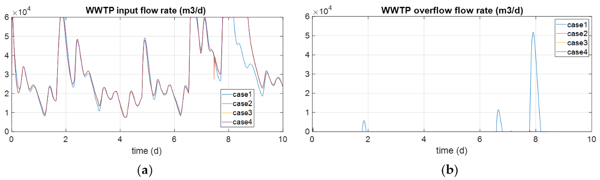
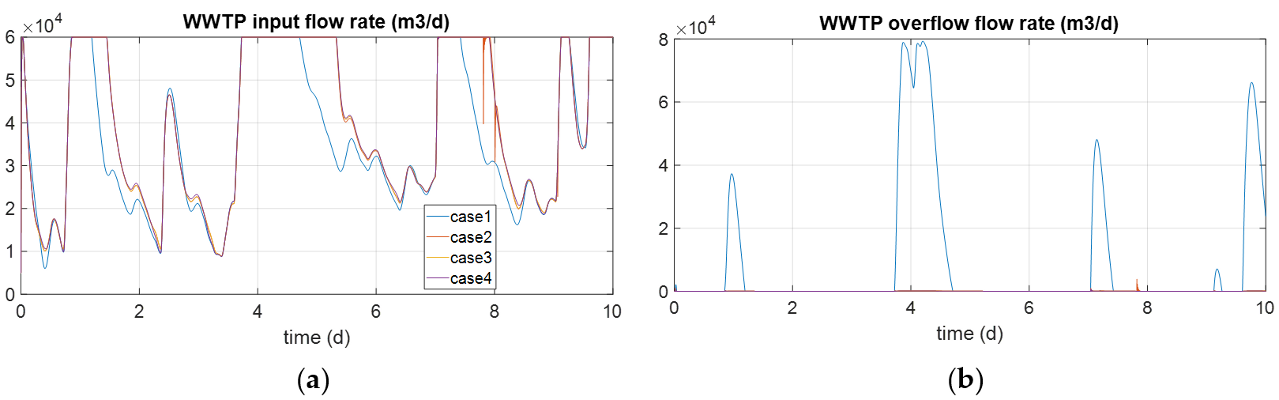
Some simulation graphic results are shown below for scenario 1. As can be seen in Figure 12, the inflow to WWTP is very similar (b), as well as the overflow flow rate (a), except in the case without control. The differences between the cases considered are better revealed in the numerical results of

Table 5. Numeric results for scenario 1.

Data	No Control	Decentralized MPC	DMPC with Fuzzy Negoc.	Centralized MPC
Nov,11	0	1	1	1
Nov,2	1	1	1	1
Nov,3	1	1	1	1
Nov,4	1	1	1	1
Nov,5	0	1	1	1
Nov,WWTP	5	4	4	4
Nov	8	9	9	9
Tov,11	0	0.0583	0.0583	0.0604
Tov,2	0.0375	0.0396	0.0396	0.0396
Tov,3	0.0875	0.0813	0.0813	0.0813
Tov,4	0.2625	0.1375	0.1708	0.1604
Tov,5	0	0.1167	0.0958	0.1000
Tov,WWTP	0.8146	1.2688	1.2708	1.2563
Vov,11	0	1438.5	1440.0	1155.8
Vov,2	168.3654	175.2992	175.2992	174.8339
Vov,3	527.9974	545.3469	544.9625	542.2737
Vov,4	6224.4	4250.2	4637.8	4240.2
Vov,5	0	1722.2	1147.0	1363.9
Vov,WWTP	14376	65.3614	64.6751	66.2179
Vov	21297	6758.3	6569.7	6387.5
QWWTP	30124	31537	31556	31583
Gu	50.2067	52.5620	52.5933	52.6386
S	-	1.0983 × 1011	6.0324 × 1010	6.2001 × 1010

¹ The overflow volume in tank 1 returns to the network due to the sewer configuration. Therefore, it is not added to V_ov.

. For brevity, only tank 4 level (a) and outflow set point (b) in each case are shown in Figure 13.

The evolution of the water level in tank 4 can be seen together with the reference proposed by the upper layer of the hierarchical controller. The reference tracking is considerably better for cases 2, 3, and 4 than for case 1 (without control). Therefore, if no control is applied, more overflow is produced at the inlet of the WWTP, because not enough water is maintained in the sewer tanks. The controlled cases also improve the total number of overflows at the inlet of the WWTP and the total volume of overflow water (Table 4). Regarding the inlet flow to the WWTP, it is difficult to keep the nominal value q_WWTPnom, because the water received in the catchments has large variations and most of the time is not enough to reach that value. However, when control is applied, more water is stored in tank 5, allowing for a better regulation of the nominal value of the WWTP inlet flow (Figure 12a).

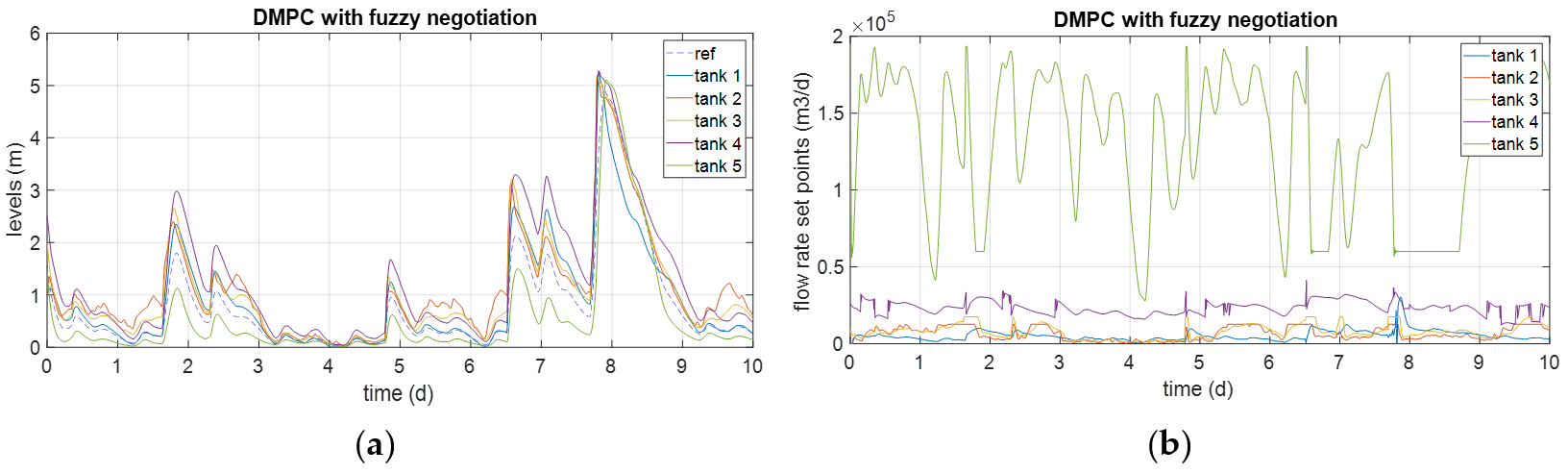
In Figure 14, level (a) and output flow rate set point (b) can be observed for every tank in case 3, corresponding to a Distributed MPC with fuzzy negotiation. Levels are represented together with the reference level calculated at each instant according to (22). Some of them are closer than others to the reference value to minimize the volume of overflowed water and optimize the inflow to the WWTP.

For scenario 2, some graphic results are shown in Figure 15 and Figure 16.

The results for scenario 2 present a larger number of overflow events (N_ov) and a larger overflow (V_ov) due to the increase of the water received (disturbances). On the other hand, the usage of the WWTP (G_u) and the Q_WWTP average are due to the larger availability of water to keep the WWTP working close to the nominal operation point.

In Table 5 (for scenario 1) and

Table 6. Numeric results for scenario 2.

Data	No Control	Decentralized MPC	DMPC with Fuzzy Negoc.	Centralized MPC
Nov,11	3	3	3	3
Nov,2	3	3	3	3
Nov,3	4	4	4	4
Nov,4	4	4	4	4
Nov,5	2	2	2	2
Nov,WWTP	6	6	6	6
Nov	22	22	22	22
Tov,11	0.1750	0.3958	0.4021	0.4333
Tov,2	0.1750	0.3750	0.3833	0.5000
Tov,3	0.5958	0.4958	0.5292	0.6188
Tov,4	1.5521	0.9063	0.9938	0.9562
Tov,5	0.2687	0.8583	0.8042	0.8146
Tov,WWTP	2.2729	3.5333	3.5646	3.5583
Vov,11	3457.7	19,497	19,585	17,682
Vov,2	1299.1	2777.8	2770.4	3403.4
Vov,3	5996.7	5891.4	5837.9	5876.5
Vov,4	54707	42,133	48,679	42,387
Vov,5	8826.6	57,569	50,456	55,440
Vov,WWTP	89,632	260.8809	237.2997	241.2602
Vov	160,460	108,630	107,980	107,350
QWWTP	35,830	39694	39725	39,774
Gu	59.7160	66.1573	66.2077	66.2894
S	-	2.0269 × 1011	6.9150 × 1010	7.1428 × 1010

¹ The overflow volume in tank 1 returns to the network due to the sewer configuration. Therefore, it is not added to V_ov.

(for scenario 2), the performance indices presented in Section 2.2 are presented for the four cases. Case 1 (without control) is the worst for all indices, as expected, and the centralized MPC presents the best performance for indices such as the average flow entering the WWTP (Q_WWTP), the degree of usage of WWTP (G_u), and the total volume overflow (V_ov). However, the DMPC with fuzzy negotiation does not show an important decrease of those indices, with the advantage of using local simpler models and optimization problems. Moreover, the use of DMPC provides the smallest S, due to the smoothing effect of the fuzzy sets considered for negotiation. The case of Decentralized MPC provides the worst performance indices because the local controllers do not exchange information and the existing coupling in the network is not considered.

Finally, to analyze the influence of the fuzzy set design on the performance of the distributed control algorithm, the location of the fuzzy sets has been changed according to

Table 7. Fuzzy sets definition for different DMPC cases.

	$\mathit{\mu }\left({\overline{\mathit{q}}}_{\mathit{W}\mathit{W}\mathit{T}\mathit{P}}\right)$			$\mathit{\mu }\left({\overline{\mathit{q}}}_{\mathit{o}\mathit{v}}\right)$
Case	a	b	c	a	b
DMPC 1	56,000	58,000	60,000	1000	2000
DMPC 2	54,000	56,000	58,000	1000	2000
DMPC 3	58,000	60,000	62,000	1000	2000
DMPC 4	56,000	58,000	60,000	0000	1000
DMPC 5	56,000	58,000	60,000	2000	3000

, but their shape was preserved. Results are presented in

Table 8. Numeric results for scenario 1 varying DMPC fuzzy sets.

Data	DMPC1	DMPC2	DMPC3	DMPC4	DMPC5
Tov,11	0.0583	0.0583	0.0583	0.0583	0.0583
Tov,2	0.0396	0.0396	0.0396	0.0396	0.0396
Tov,3	0.0813	0.0813	0.0813	0.0813	0.0813
Tov,4	0.1708	0.1708	0.1583	0.1708	0.1708
Tov,5	0.0958	0.0958	0.1042	0.0958	0.0958
Tov,WWTP	1.2708	1.2708	1.2646	1.2708	1.2708
Vov,11	1440.0	1440.0	1461.0	1440.0	1440.0
Vov,2	175.2992	175.2992	175.3114	175.2992	175.2992
Vov,3	544.9625	544.9625	545.1972	544.9625	544.9625
Vov,4	4637.8	4637.8	4417.7	4637.8	4637.8
Vov,5	1147.0	1147.0	1392.6	1147.0	1147.0
Vov,WWTP	64.6751	64.6751	65.2556	64.5500	64.6878
Vov	6569.7	6569.7	6596.1	6569.5	6569.7
QWWTP	31,556	31,556	31,553	31,556	31,556
Gu	52.5933	52.5933	52.5889	52.5933	52.5933
S	6.0324 × 1010	6.0144 × 1010	6.0583 × 1010	6.0322 × 1010	6.0325 × 1010

¹ The overflow volume in tank 1 returns to the network due to the sewer’s configuration. Therefore, it is not added to V_ov.

. The DMPC1 and DMPC2 cases present practically identical results. Therefore, it follows that the influence of the position variation of the fuzzy sets is negligible. By comparing DMPC2 and DMPC3, it can be seen that the degree of usage of the WWTP is slightly smaller in the case of DMPC3 because the center of the fuzzy set has been moved to the WWTP constraint of 60,000 m³/d. By comparing DMPC3 and DMPC4, the overflow (V_ov) is larger for DMPC4 because the fuzzy set considers as negligible overflows of larger amount. Anyway, the results are very similar because the limits of the fuzzy sets are very next to each other.

9. Conclusions

In this document, a DMPC with fuzzy negotiation has been developed and applied to a sewer network, with good results in comparison with centralized and decentralized MPC. As expected, centralized MPC provides the best performance because the controller makes use of the full linearized model of the process. However, the DMPC performance is similar, dealing with simpler local optimization problems and other common advantages of distributed strategies, such as fault tolerance. As for the comparison with a decentralized MPC, where there is no communication among agents, the negotiation improves the results significantly. The methodology developed is based on linearized local models, which further simplifies the MPC optimization problems solved by each subsystem. Moreover, the fuzzy negotiation allows for the inclusion of expert process knowledge by means of fuzzy sets whose precise shape is defined by flows and intuitive fuzzy rules that can be adjusted depending on the specific needs of the network. In this way, no other cumbersome tuning parameters have been added to the negotiation procedure.

The methodology proposed here is currently valid only for two subsystems, but it can easily be extended to a larger number of local systems due to the use of standard sectorization techniques and introducing, for example, the concept of neighborhood, where the coupling among subsystems is high. Due to the use of the benchmark [3], it would also be possible to include the concentration of the most relevant pollutants in the procedure. Although UDS control is mainly commanded by flow and level dynamics, due to the irrelevant biological degradation of pollutants in the sewer, future works will consider some of them, e.g., the Total Suspended Solids concentration, with the aim of improving the industrial applicability of the controller.