Hybrid Modeling for Simultaneous Prediction of Flux, Rejection Factor and Concentration in Two-Component Crossflow Ultrafiltration

Abstract

Ultrafiltration is a powerful method used in virtually every pharmaceutical bioprocess. Depending on the process stage, the product-to-impurity ratio differs. The impact of impurities on the process depends on various factors. Solely mechanistic models are currently not sufficient to entirely describe these complex interactions. We have established two hybrid models for predicting the flux evolution, the protein rejection factor and two components’ concentration during crossflow ultrafiltration. The hybrid models were compared to the standard mechanistic modeling approach based on the stagnant film theory. The hybrid models accurately predicted the flux and concentration over a wide range of process parameters and product-to-impurity ratios based on a minimum set of training experiments. Incorporating both components into the modeling approach was essential to yielding precise results. The stagnant film model exhibited larger errors and no predictions regarding the impurity could be made, since it is based on the main product only. Further, the developed hybrid models exhibit excellent interpolation properties and enable both multi-step ahead flux predictions as well as time-resolved impurity forecasts, which is considered to be a critical quality attribute in many bioprocesses. Therefore, the developed hybrid models present the basis for next generation bioprocessing when implemented as soft sensors for real-time monitoring of processes.

1. Introduction

Membrane separation is a unit operation used in virtually all bioprocesses. One prominent type, crossflow ultrafiltration, is widely used from cell harvest and virus clearance approaches to product concentration steps. In downstream processing of biopharmaceuticals, ultrafiltration (UF) is commonly applied for concentration and buffer exchange after the capture step. It is also applied after virus filtration in single-pass mode to concentrate the sample before it is loaded onto the polishing chromatography, or after polishing to reach the final conditions for product formulation [1]. These process steps entail varying ratios of process and impurities to product concentration.

Modeling of process steps is of increasing importance for bioprocesses. Such process models increase understanding of processes, facilitate the discovery of optimal process conditions and are indispensable for model predictive control. The latter is a cornerstone of Quality by Design and Process Analytical Technology, which is recommended by authorities for biopharmaceutical production. The right balance of model complexity and usability is crucial to employ such models effectively for different unit operations.

To simplify the modeling of downstream processes, a common assumption is to reduce the overall sample composition down to a single target molecule. Coefficients and parameters used in mechanistic models, such as mass transfer models, are often approximated, taking only the target molecule into account. Such models may be limited if the sample contains high levels of impurity.

For some process steps, such as polishing chromatography [2] or ultra/diafiltration [3,4] before formulation, this assumption of one-component solutions is realistic, since the product is already of high purity at this process stage. For earlier process steps, however, this simplification deviates substantially from reality and can lead to erroneous models, e.g., for filtration steps after the capture step. Here, the neglected presence of host cell proteins [5], DNA [6], or protein aggregates [7] can strongly distort the prediction of the model, since effects like membrane fouling and interactions between the product and impurities are not considered. In more complex mechanistic models, if the impurities are well characterized, such effects can be considered. For example, for crossflow filtration, a hard sphere-based mixture model, including multiphase computational fluid dynamics and concentration polarization, was applied to a whey protein solution, leading to a permeate flux prediction error within 20% [8]. Other work has shown that mechanistic models of pore blockage and cake filtration can also predict filter fouling during virus filtration, as a function of the protein of interest, virus and membrane [9]. The initial and late stage of the filtration, however, was dominated by different mechanisms, rendering it difficult to build a valid model for the entire process. The influence of two components on (crossflow) UF was found to affect the process in different ways, from strong [10] to weak [11] to varying [5,12,13,14] protein-protein (or protein-membrane) interactions. To account for the highly different effects of all components on the process, the experimental part of data generation to estimate the parameters for mechanistic models might become very labor-intensive and the calculations rather complex. Further, if the overall behavior of the process changes because of varying concentrations of impurities, the assumptions of mechanistic models might not hold, to the detriment of the prediction.

One advantage of machine learning supported modeling approaches is that the effects of the impurity on flux and membrane fouling do not need to be fully quantified by the operator [15]. The quantification of these phenomena is performed by machine learning tools, such as an artificial neural network (ANN) [16]. Hybrid models combine the advantages of data-driven black box models (such as ANNs), correlating input with output variables (such as the concentration of impurity with the decrease in flux) with knowledge-based mechanistic models (white box models) derived from conservation of kinetic laws [17]. Hybrid models have been applied to bioprocesses for upstream [18] and downstream applications [19,20].

To compare the predictive power of a model concerning the training space, two terms are often used: interpolation and extrapolation. Interpolation allows the model to make predictions for parameters that lie within the range of training experiments. A model with good interpolation capabilities can make predictions with fewer training observations, since it is able to make reliable estimates of the spaces between the observations. A model with poor interpolation capabilities requires more granular coverage of the training space to make accurate predictions of test experiments. Extrapolation (also called range extrapolation) describes the extent to which a model can make predictions if the tested input parameters are outside the training space. A model with good extrapolation capabilities can make accurate predictions for parameters beyond the training space. A detailed explanation of interpolation and extrapolation in hybrid modeling is given in [21].

Recently, we have shown the benefits of hybrid modeling for the prediction of UF flux evolution. However, this previous model was only established for a one-component system [22]. In the present study, we extended the hybrid model to describe the impact of a modeled protein impurity on the decrease of the permeate flux over time in crossflow UF including the rejection behavior of the product and the impurity. This enables the operator to gain a more detailed understanding of the process. In addition, the impurity concentration is a critical quality attribute (CQA) in almost all manufacturing bioprocesses and if it is too high, the produced batch must be discarded. The presented hybrid models can predict the impurity concentration up front, and potentially minimizes the risk of batch rejection.

Product and impurity were mimicked with different ratios of bovine serum albumin (BSA) to lysozyme concentrations in the starting solution. BSA and lysozyme exhibit different physicochemical properties to facilitate separation and quantification. While BSA was fully retained by the membrane, lysozyme was only partially retained, rendering the predictions of the permeate flux over time even more complex. In a first assessment, we compared the abilities of the well-established mechanistic stagnant film model (SFM) and the recently established one-component hybrid to predict the filtration progress of a two-component solution. Further, we presented two hybrid model structures to predict the evolution of permeate flux and protein concentration of product and impurity by multi-step ahead predictions. One hybrid model included a static lysozyme rejection factor (R_Lys), while the other updated R_Lys dynamically in an iterative way. These model outputs were influenced by the transmembrane pressure (TMP), crossflow velocity (CF), the initial BSA concentration c_B,BSA and lysozyme bulk concentration c_B,Lys. Finally, these novel hybrid model structures were compared to the SFM regarding flux and concentration prediction.

2. Materials and Methods

2.1. Equipment and Chemicals

All UF experiments were performed on an ÄKTA Crossflow system (Cytiva, Marlborough, MA, USA) controlled by UNICORN 5.31 software. The reservoir tank held up to 1100 mL of bulk solution. The system featured an inline pH probe and UV monitor on the permeate side and a pressure-based reservoir level sensor. The experiments were performed with a Sartocon Slice Hydrosart Cassette hydrophilic, stabilized cellulose-based membrane (Sartorius AG, Göttingen, Germany) with a membrane area of 200 cm². The model proteins were BSA and lysozyme (A2153 and L6876, both purchased from Sigma-Aldrich, St. Louis, MO, USA). The molecular weight cutoff (MWCO) of the membranes was 30 kDa, chosen so that BSA (66 kDa) was fully retained and lysozyme (14 kDa) was partially retained. BSA and lysozyme were chosen to mimic the protein of interest and process-related impurities, respectively. A filtration buffer of 50 mM phosphate-buffered saline (PBS), pH 8, was used.

2.2. Training and Test Data Generation

For the training experiments, the bulk reservoir was filled with 1000 mL of the lowest bulk BSA and/or lysozyme concentration c_B,BSA and c_B,Lys (see

Table A1. Summary of all training data including measured c_B,BSA, c_B,Lys, and observed flux.

Training Set	Observation	cB,Lys [g/L]	cB,BSA [g/L]	Flux at TMP 0.8 bar [LMH]	Flux at TMP 1.3 bar [LMH]	Flux at TMP 1.8 bar [LMH]	Flux at TMP 2.3 bar [LMH]	Flux at TMP 2.8 bar [LMH]
1	100	0.28	3.77	87.6	113.3	121.0	121.5	119.1
		0.5	8.48	78.0	93.3	96.3	95.6	93.4
		0.76	14.38	70.1	80.5	81.6	80.0	77.7
		1.51	24.68	60.7	67.5	67.5	65.9	63.9
		2.3	48.72	46.8	50.7	50.1	48.6	47.1
		3.81	77.93	34.0	36.6	36.2	35.1	34.0
	200	0.28	3.77	92.9	136.3	157.6	164.5	164.2
		0.5	8.48	89.3	121.2	131.9	132.7	130.3
		0.76	14.38	82.8	106.5	112.3	111	108.3
		1.51	24.68	74.2	91.1	93.5	91.6	88.8
		2.3	48.72	59.2	68.6	69.2	67.1	64.7
		3.81	77.93	43.3	49.3	49.4	47.8	46.2
	300	0.28	3.77	92.0	143.4	178.3	194.8	199.8
		0.5	8.48	90.2	133.8	155.6	161.5	161.1
		0.76	14.38	85.6	121.5	135.2	136.9	134.7
		1.51	24.68	78.8	106.2	114.0	113.4	110.7
		2.3	48.72	65.1	82.2	85.1	83.2	80.6
		3.81	77.93	48.4	59.2	60.4	58.9	56.9
2a	100	3.19	-	97.6	150.1	195.1	232.6	260.6
		4.73	-	97.9	146.5	186.1	218.2	244.8
		8.11	-	97.6	144.7	181.1	209.5	235.8
		11.99	-	96.8	142.2	176.8	205.2	231.8
		23.79	-	95.0	137.5	171.0	199.1	221.8
		32.95	-	85.7	124.9	152.3	172.4	187.2
	200	0.39	-	98.3	151.9	196.6	233.6	264.2
		0.44	-	99	150.8	192.2	224.3	252.4
		0.53	-	98.3	148.7	187.9	218.9	244.8
		0.72	-	98.3	146.9	184.7	215.3	241.6
		0.9	-	96.8	143.3	178.9	208.4	232.9
		1.48	-	89.3	128.9	160.9	186.5	204.1
	300	3.19	-	97.2	152.28	198.36	236.52	267.84
		4.73	-	97.56	150.84	195.48	229.68	258.12
		8.11	-	96.84	149.4	192.24	225	252.36
		11.99	-	96.84	148.32	189.36	222.12	249.84
		23.79	-	96.12	145.08	183.6	215.28	240.84
		32.95	-	86.76	129.96	165.6	192.6	212.76
2b	100	3.19	-	86.0	113.8	121.0	115.6	105.5
		4.73	-	67.3	81.0	84.2	82.4	79.9
		8.11	-	59.8	69.8	71.6	70.6	68.8
		11.99	-	55.1	62.6	63.4	61.9	60.5
		23.79	-	45.7	50.0	49.7	47.9	46.8
		32.95	-	36.0	37.8	36.4	35.3	34.2
	200	3.19	-	88.2	121.7	135.7	137.9	134.3
		4.73	-	74.5	96.1	105.8	108.4	108.0
		8.11	-	67.7	85.7	92.9	94.3	93.6
		11.99	-	63.0	78.5	83.9	84.2	82.8
		23.79	-	54.0	64.8	67.0	65.5	63.4
		32.95	-	43.9	50.0	49.7	47.9	46.8
	300	3.19	-	85.0	121.0	140.0	148.7	151.2
		4.73	-	74.9	102.6	117.7	125.6	128.5
		8.11	-	69.5	93.2	105.8	111.6	113.0
		11.99	-	65.5	87.5	97.6	100.8	100.8
		23.79	-	57.2	73.8	79.2	79.6	78.1
		32.95	-	50.0	62.6	64.8	-	-
3a	100	-	3.65	90.8	119.6	131.9	136.5	138.3
		-	7.45	84.9	106.8	114.8	117.4	117.2
		-	14.65	76.6	92.4	97.0	97.3	96.4
		-	20.06	68.2	82.1	85.5	85.1	83.3
		-	24.4	67.2	78.7	82.0	82.0	80.8
		-	44.78	53.2	61.4	63.2	62.9	61.6
	200	-	3.65	97.9	144	171.7	185.4	191.5
		-	7.45	96.1	135	154.4	162	164.5
		-	14.65	90.4	119.9	132.1	135.7	135
		-	20.06	81.4	108.4	118.4	119.9	118.1
		-	24.4	82.1	104.8	113	114.5	113
		-	44.78	67.3	82.4	86.8	86.8	85
	300	-	3.65	98.4	151.4	190.8	214.9	228.5
		-	7.45	98.6	147.2	178.4	194.4	201.0
		-	14.65	93.8	134.4	155.9	164.9	167.2
		-	20.06	87.5	124.9	143.4	149.2	149.0
		-	24.4	87.6	120.8	136.0	141.1	141.3
		-	44.78	74.6	97.9	106.1	107.9	106.8
3b	100	-	70.12	40.7	46.4	47.3	46.6	45.5
		-	80.15	39.4	45.5	46.9	46.6	45.8
		-	131.69	24.0	28.8	29.9	29.6	29.0
		-	179.95	13.6	18.1	19.6	19.7	19.7
		-	231.67	6.3	10.9	13.1	13.8	13.7
		-	277.25	0.0	5.5	7.7	8.8	9.4
	200	-	70.12	53.6	64.1	66.2	65.5	63.4
		-	80.15	50.8	61.2	63.7	63.4	62.6
		-	131.69	31.8	38.9	40.3	40	39.2
		-	179.95	17.3	23.5	25.7	26	25.7
		-	231.67	7.2	13.8	16.3	17.4	17.5
		-	277.25	5.9	9.4	10.8	-	-
	300	-	70.12	62.6	79.0	83.3	82.6	63.5
		-	80.15	58.2	73.3	78.0	78.3	62.5
		-	131.69	37.1	46.8	49.5	49.3	39.2
		-	179.95	19.5	27.5	30.3	30.9	25.7
		-	231.67	-	-	-	-	17.5
		-	277.25	-	-	-	-	-

). The following two steps were then alternated. First, the TMP and CF were increased stepwise, while the permeate was redirected to the feed reservoir to keep the protein concentration c_B constant. For each combination of TMP and CF, the permeate flux was recorded. Second, the sample was concentrated until the next desired c_B was reached. These two steps were repeated at all concentrations given in Table A1. A total of 90 equilibrium fluxes were recorded for different concentrations and combinations of TMP and CF. Our previous work with a one-component system [22] showed that this training set size was sufficient to develop a well-trained hybrid model with accurate flux predictions. A detailed summary of all scouted TMPs, CFs, c_Bs and recorded fluxes is given in Table A1. Samples were taken after each concentration step for offline measurement. A more detailed description of the methodology for the training experiment is given in an earlier publication [22].

During the test experiments, samples were taken from the retentate and permeate. The measured retentate and permeate concentrations were used to calculate the rejection factor R of the model proteins. A summary of the performed test sets is provided in

Table A2. Summary of the test sets with varying initial c_Bs, CF, and TMP.

Test Set Number	TMP [bar]	CF [mL/min]	Initial cB,BSA [g/L]	Final cB,BSA [g/L]	Initial cB,Lys [g/L]	Final cB,Lys [g/L]
1	1.8	200	4.00	78.11	0.28	4.36
2	1.8	200	3.79	62.48	0.50	6.16
3	2.8	300	3.82	54.95	0.32	4.35
4	2.5	280	4.56	97.59	0.28	3.52
5	1.6	230	5.97	132.81	0.15	1.96
6	1.4	270	8.80	162.45	0.19	2.79
7	2.0	350	3.62	73.62	0.34	4.65
8	1.8	260	2.38	45.42	0.57	6.82
9	1.8	200	6.68	132.70	0.00	0.00

.

2.3. Concentration Polarization Correction

When concentrating the sample throughout the training experiments, we observed that the measured c_B,BSA was lower than the expected concentration calculated from permeate volume (V_P) and mass balance. The difference between observed and calculated concentration increased with concentration (see Figure A3B). This was because the concentration polarization (CP) layer—the protein gradient that forms on the surface of the membrane—increased with c_B,BSA. This deviation was considered for the test experiments by employing a quadratic polynomial function (Equation A1) and used to correct the calculated c_B,BSA.

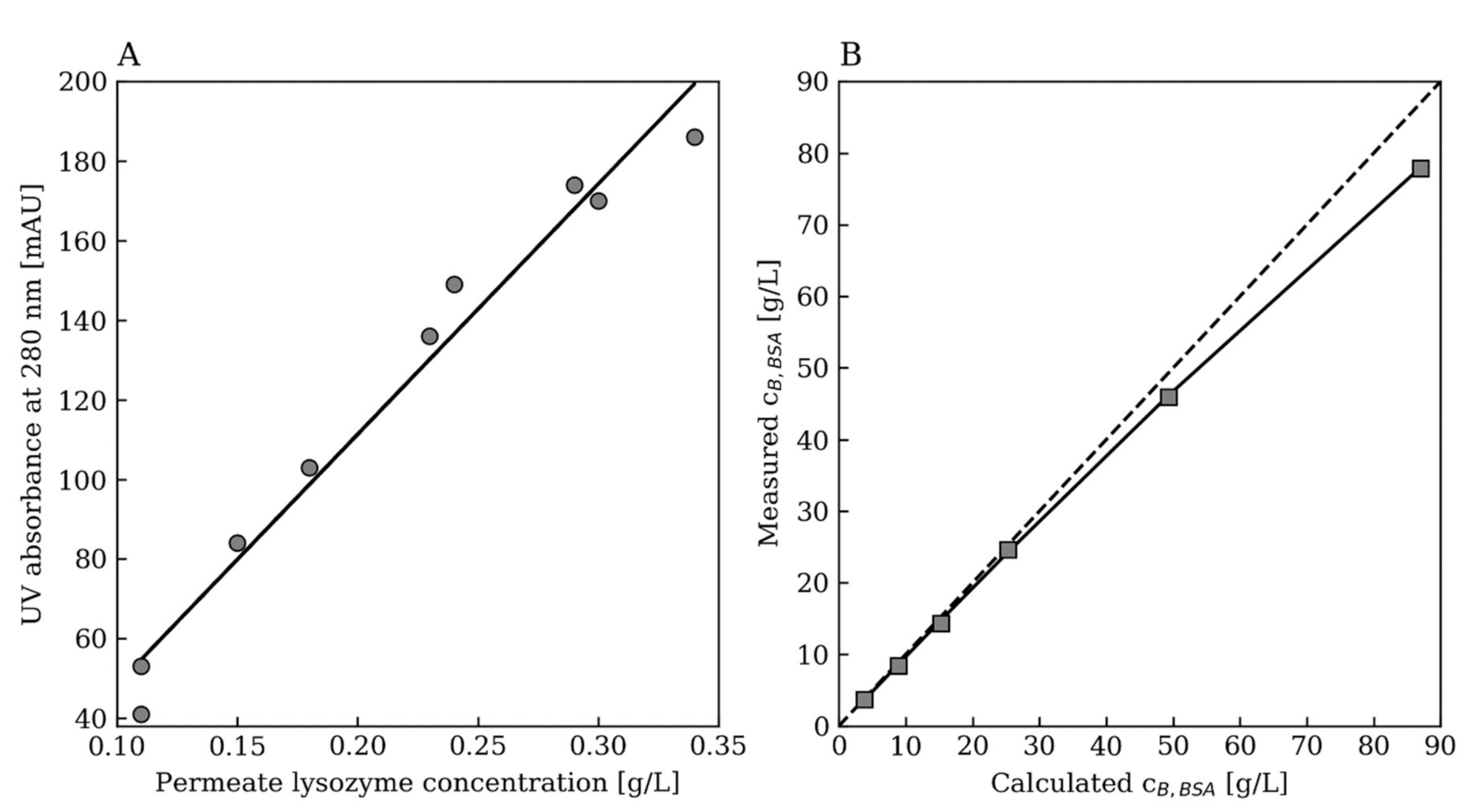
2.4. Protein Quantification

BSA and lysozyme concentrations were determined with an analytical high-performance size-exclusion chromatography (SEC-HPLC) using a TSKgel G3000SWXL column (5 µm, 7.8 × 300 mm; TOSOH, Shiba, Tokyo, Japan). The separation was performed under isocratic conditions with 50 mM sodium phosphate, 200 mM NaCl, pH 6.5 as running buffer at a flow rate of 0.4 mL/min. Samples were diluted to a final concentration of 0.1 to 1.0 g/L using 50 mM PBS, pH 8 and filtered through a 0.22 μm Millex-GV Filter (Merck Millipore, Billerica, MA, USA) prior to analysis. The injection volume was 10 μL per sample. Due to the difference in the size of BSA and lysozyme, the peaks were fully separated and could be quantified independently, using standard calibrations from BSA and lysozyme stock solutions.

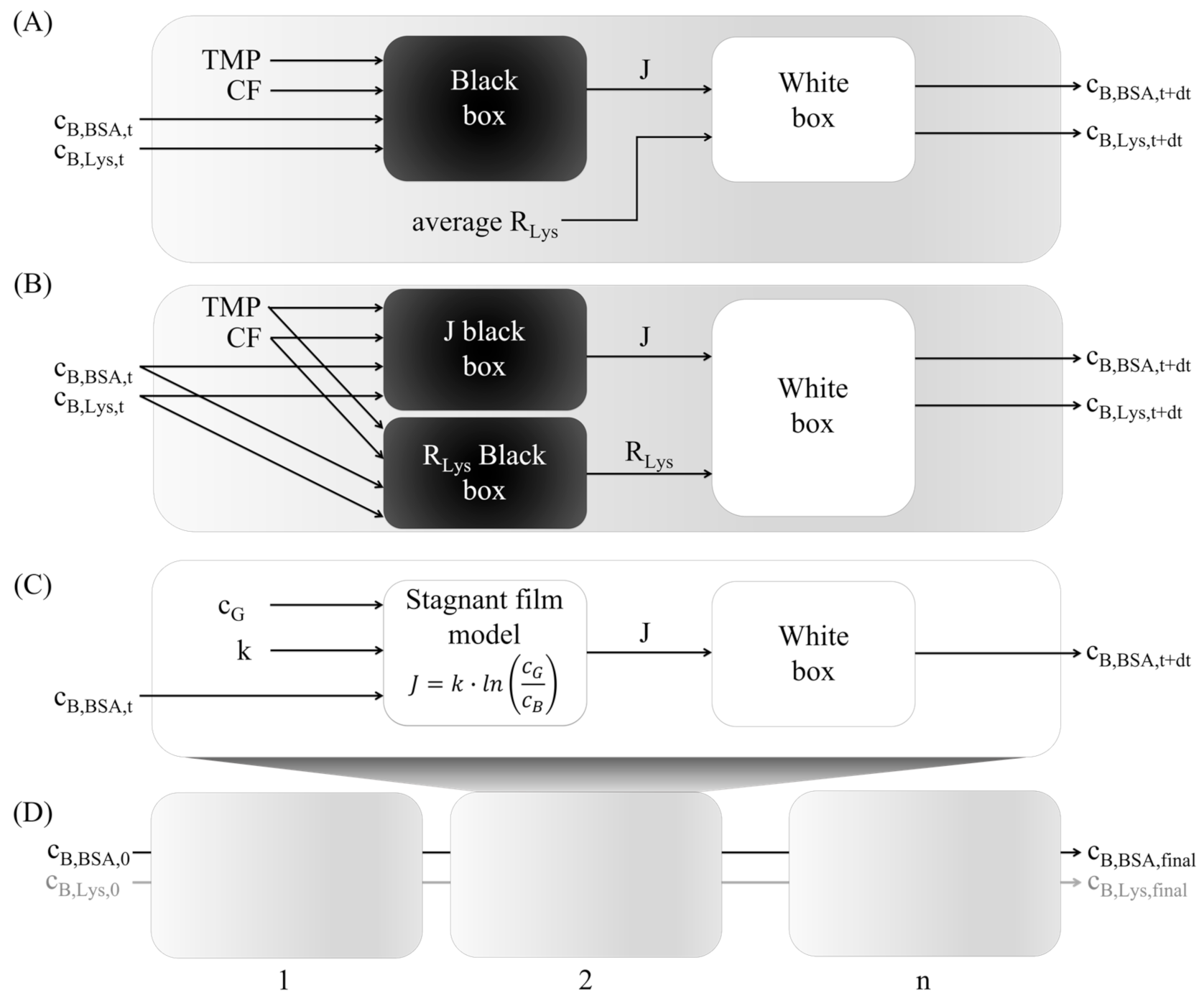
2.5. Hybrid Modeling

2.5.1. Black Box Model

The black box inside the first hybrid model (HM 1) aimed to predict the flux based on the combination of inputs parameters: TMP, CF and the bulk protein concentrations of BSA and lysozyme, c_B,BSA and c_B,Lys, respectively. In the second hybrid model (HM 2), an additional black box was employed to predict the rejection factor of lysozyme R_Lys (Figure 1B). An ANN was utilized for this purpose and optimized by varying the number of hidden nodes from 1 to 7. The ANN was set up with the feedforwardnet function and trained with the trainbr function, using MATLAB 2018b. A detailed description is the ANN structure and optimizer function is given in the Appendix A.

2.5.2. White Box Model

The white box model is the mechanistic part of the hybrid model and consisted of a mass balance. The incrementally decreasing bulk volume (dV_B in Equation (1)) was derived from the permeate flux (J), which is the output of the black box, and the membrane area (A). The rejection factor R for component i was calculated with Equation (2), considering the concentration of i in both the retentate (c_R; in crossflow filtration c_R is equal to c_B) and the permeate (c_P). Equation (1) and Equation (2) were used to predict c_B of each component and Equation (3) to calculate the V_B after dt.

$$\frac{{\mathrm{dV}}_{\mathrm{B}}}{\mathrm{dt}}=-\mathrm{A}·\mathrm{J}$$

(1)

$${\mathrm{R}}_{\mathrm{i}}=1-\frac{{\mathrm{c}}_{\mathrm{P},\mathrm{i}}}{{\mathrm{c}}_{\mathrm{R},\mathrm{i}}}$$

(2)

$$\frac{\mathrm{d}\left({\mathrm{c}}_{\mathrm{B},\mathrm{i}}·{\mathrm{V}}_{\mathrm{B}}\right)}{\mathrm{dt}}={\left(\mathrm{A}·\mathrm{J}·{\mathrm{c}}_{\mathrm{B},\mathrm{i}}\right)}^{{\mathrm{R}}_{\mathrm{i}}}$$

(3)

2.5.3. Training and Test Data

R_Lys was calculated from the training set with the UV absorbance at 280 nm on the permeate side. A separate lysozyme training run was performed to correlate the UV signal at 280 nm with the permeate concentration determined by SEC-HPLC. The correlation curve (Figure A3A) with an R² of 0.97 was used to calculate c_P,Lys, and subsequently R_Lys for all observations of the training set was used to train the black box.

The observed flux and R_Lys were compared to the predictions of the hybrid models using the normalized root-mean-square error (NRMSE)

$$\mathrm{NRMSE}=100·\frac{\sqrt{\frac{1}{\mathrm{n}}{\sum }_{\mathrm{i}=1}^{\mathrm{n}}{\left({\mathrm{y}}_{\mathrm{i}}-{\hat{\mathrm{y}}}_{\mathrm{i}}\right)}^2}}{{\mathrm{y}}_{\max }-{\mathrm{y}}_{\min }}$$

(4)

where n is the number of overserved fluxes y_i and the corresponding predicted fluxes ${\widehat{y}}_i$. The normalization y_max−y_min allows a fair comparison of various fluxes due to different concentrations and process parameters.

2.5.4. Multistep-Ahead Hybrid Model

The structures of the investigated hybrid model are given in Figure 1. The first and simplest HM 1 (Figure 1A) assumed a constant R_Lys of 0.77 for all test sets based on the weighted average of all permeate and retentate concentrations samples taken throughout the training experiment. The weighted average considered the variation in c_B,Lys and sample intervals using trapezoid rule integration. For the second HM 2 structure (Figure 1B), the flux and R_Lys were predicted separately, using two different black box models. The flux and R_Lys were fed into the same white box model, which yielded the predicted c_B,BSA and c_B,Lys after a defined time increment. The developed hybrid model is capable of predicting multiple steps ahead, as depicted in Figure 1D. The multi-step ahead structure uses HM 1, HM 2 or the SFM to predict c_B,BSA and c_B,Lys for a time increment (dt). The concentrations of the first iteration were used to calculate future fluxes and c_Bs of the second iteration, and so on. Multiple iterations were performed until the desired stop criterion was reached. In our case, the stop criterion was the final retentate volume.

The presented hybrid models were used to predict the evolution of flux and R_Lys throughout the UF process. Furthermore, the models yielded a prediction for the final c_B,BSA and c_B,Lys. The final c_B,BSA and c_B,Lys predictions were compared to the final c_B,BSA and c_B,Lys measured by SEC-HPLC. The model errors were compared using the NRMSE.

Figure 2 shows a flowchart of the hybrid model methodology applied for crossflow filtration. Training experiments were performed by variations in the parameters that are expected to influence the flux. Following this, the model was trained on this training set with a defined experimental design space. The established models were applied to a validation data set that was not used for training. The model structure was optimized by varying the tuning parameters, e.g., number of nodes in an ANN and adding or removing training parameters. The model with the tuning parameters that led to the lowest error in the validation set was then applied to independent test runs with static process conditions.

2.5.5. Stagnant Film Theory

The presented hybrid models were compared to the established SFM. The SFM derives predictions from the mass transfer model described by convective transport toward the membrane and back-diffusion caused by the concentration gradient [23]. According to the SFM, the flux J is related to the bulk concentration c_B of a single component by

$$\mathrm{J}=\mathrm{k}·\ln \left(\frac{{\mathrm{c}}_{\mathrm{G}}}{{\mathrm{c}}_{\mathrm{B}}}\right)$$

(5)

where c_G is the gel layer concentration at the membrane surface and k is the mass transfer coefficient that depends on the diffusion coefficient and the thickness of the gel layer [23]. The SFM is valid in the pressure-independent region of the filtration. Since k and c_G cannot be adjusted directly during the filtration, a correlation between the adjustable parameters TMP and CF, and k and c_G was required. When plotting the flux versus log(c_B) for a constant TMP and CF, k and c_G are estimated by the slope of linear regression and c_G was estimated by extrapolating the regression line to the intersection with the abscissa (Figure A6). It has been shown that this way of calculating k yields more accurate results than the Sherwood correlation [24,25,26] and more solid predictions compared to the osmotic pressure model [27] for similar settings. To compare the SFM to the hybrid models, the black box was replaced by the SFM in Equation (5) using the parameters k and c_G instead of TMP and CF (Figure 1C). In test runs, where the TMP and CF conditions were not covered in the training set, k and c_G were estimated using linear interpolation.

3. Results and Discussion

3.1. Training Data Description

The data sets for training the hybrid models were generated from filtering BSA and lysozyme with a 30 kDa MWCO cellulose-based membrane (Hydrosart). A total of three training sets were generated covering three CFs (100, 200 and 300 mL/min) and five TMPs (0.8, 1.3, 1.8, 2.3 and 2.8 bar). The three training sets containing BSA, lysozyme and a combination of both are shown in Figure 3. In the combined training set, the protein concentration of BSA c_{B, BSA} ranged from 3.77 g/L to 77.93 g/L and of lysozyme c_{B, Lys} from 0.28 g/L to 3.81 g/L. The concentration ranges for all training sets are summarized in Table A1. For a better comparison of Figure 3A–D, the x-axis of Figure 3C,D are reduced. The entire graphs are given in Figure A2.

Generally, increasing bulk concentrations c_B led to lower fluxes, while increasing TMP and CF led to higher fluxes in all training sets. This is in accordance with the underlying mechanisms: higher bulk concentrations lead to higher concentrations in the boundary layer and a more prominent effect of the back diffusion along the concentration gradient. An increased TMP leads to higher convective flow towards the membrane, but also to a faster accumulation of the protein at the boundary layer. High CF decreases the thickness of the concentration polarization layer by rectangular displacement. The training set obtained from experiments using only BSA exhibited higher fluxes then the two-component training set. Additionally, the flux decreased faster during filtration of the two-component solution (Figure 3B) compared to the filtration of lysozyme only (Figure 3D). This indicated an increased membrane resistance through the fouling effect on the Hydrosart membrane caused by lysozyme. Being smaller than the pores, lysozyme adsorbed at the inner pore channels [28,29] and reduced its diameter and subsequently the flux through the membrane and the membrane’s selectivity.

The two-component training set (Figure 3A,B) was used to train the black box of the hybrid models and to obtain the mechanistic model parameters k and c_G. The data set with lysozyme solely (Figure 3D) was used for two reasons: first, to investigate the effect of TMP and CF on the permeability of lysozyme and whether R_Lys had to be recalculated for varying input parameters (Figure A5); second, to correlate the permeate lysozyme concentration with the UV signal on the permeate side. This correlation was used to calculate R_Lys (Equation (2)) for each observation of the combined training set (Figure 3A,B), using solely the permeate UV signal. Another training experiment was performed with BSA solely (Figure 3C). The observed fluxes and estimated SFM parameters k and c_G were used to investigate model behavior and error when lysozyme was present in the test set but absent in the training set.

3.2. Comparison of the Hybrid Models to the Stagnant Film Theory

The optimal ANN structure in the hybrid models was determined by varying the number of hidden nodes from one to seven and recording the average error of 20 repetitions on the training set. The ANN with four hidden nodes yielded the lowest NRMSE for both HM 1 and HM 2, with an average of 3.4% NRMSE. Higher numbers of hidden nodes led to an error increase due to training set overfitting (Figure A1).

With the SFM, the flux can only be modeled for a one-component system; no adaptations for a two- or multi-component system have been published in the literature so far. In the following, BSA was assumed to be the only component since its concentration was four to 46 times higher than lysozyme in the test runs (Table A2). The k and c_G values of BSA, however, change in the presence of lysozyme. To allow a fair comparison between the hybrid models (which can incorporate multiple components as inputs) and the SFM, both sets of k and c_G were evaluated. Both experiments were carried out with BSA alone. The combination of BSA with lysozyme was used for flux prediction and the results were compared to the prediction of the hybrid models.

The hybrid model trained solely on BSA (Figure 4, red dotted line) and the SFM using k and c_G based solely on BSA (Figure 4, dark grey dot-dashed line) were able to predict a UF process with only BSA present (Figure 4A, black line), but failed to predict the UF flux of BSA and lysozyme (Figure 4B, black line). The latter failed due to membrane fouling by lysozyme and therefore the reduced flux and prolonged process times could not be described by any of these models.

In contrast, the hybrid model trained with BSA (Figure 3C) and BSA with lysozyme (Figure 3A,B) training runs (Figure 4, blue dashed line) were able to predict both UF processes: BSA solely and BSA with lysozyme (Figure 4, black lines). These results showed that already low amounts of lysozyme drastically changed the initial flux and flux evolution of the UF process and that incorporating both components in the model was essential for accurate predictions. On the contrary, SFM based on the training run containing BSA with lysozyme was also able to predict the two-component test run well (Figure 4B, light grey dot-dot-dashed line), but showed a drastic offset when predicting a test run with only BSA (Figure 4A, light grey dot-dot-dashed line). The k values from the two-component training set (

Table A5. Mass transfer coefficient k and gel concentration c_G for SFM based on BSA (left) and BSA with lysozyme (right).

k based on BSA					k based on BSA with lysozyme
		Feedflow [mL/min]					Feedflow [mL/min]
		100	200	300			100	200	300
TMP [bar]	0.8	47.36	36.23	31.63	TMP [bar]	0.8	17.61	33.84	14.03
	1.3	54.67	41.97	32.33		1.3	25.03	36.12	27.92
	1.8	54.51	42.14	30.13		1.8	27.59	36.75	39.06
	2.3	53.40	41.63	28.99		2.3	28.11	38.22	44.73
	2.8	53.75	42.97	27.95		2.8	27.70	38.58	46.84
cG based on BSA					cG based on BSA with lysozyme
		Feedflow [mL/min]					Feedflow [mL/min]
		100	200	300			100	200	300
TMP [bar]	0.8	277.83	303.41	279.25	TMP [bar]	0.8	665.40	280.12	4421.42
	1.3	302.79	330.45	323.30		1.3	355.06	312.56	887.24
	1.8	322.39	345.88	355.30		1.8	288.49	277.52	419.22
	2.3	332.29	353.74	369.46		2.3	264.69	273.21	304.56
	2.8	323.99	327.45	378.28		2.8	256.72	252.80	263.97

) were generally lower than those calculated from solely BSA, since membrane fouling due to lysozyme was assumed. In the absence of lysozyme, however, no membrane fouling occurred and the flux for the same c_B,BSA was higher.

In summary, the HM could predict both scenarios, since the varying concentration of lysozyme and its influence on the membrane fouling was integrated into the black box. However, the SFM only predicted one scenario well, depending on which k and c_G were used. For the following two-component predictions, the SFM parameters were based on the two-component training set.

3.3. Comparison of Hybrid Model Performance

To further investigate both the interpolation and extrapolation capability of both HMs and the SFM model, a series of test runs were conducted under conditions that were partially not covered by the training sets. To test the hybrid models based on the two-component training set, additional test runs on BSA solutions spiked with lysozyme were performed. The two established hybrid model structures were compared for their R_Lys, flux and final c_B predictions individually. R_Lys effects the in-process c_B,Lys prediction and subsequently the flux and final c_B,Lys. Additionally, the two hybrid models were compared to the SFM in terms of flux and c_B,BSA prediction. c_B,Lys, and R_Lys could not be compared, since SFM can be applied to one-component only.

The test data consisted of nine UF runs performed at different TMP, CF, initial c_B,BSA and c_B,Lys conditions. Test runs 1−4 were performed within the training space. This meant that TMP and CF were within the training parameters (Figure 5A, blue area) and the initial c_B,BSA, and c_B,Lys was higher than the initial training concentrations (Figure 5B, blue area). The test runs 1, 2 and 9 were performed in the center of the TMP and CF training space (Figure 5A), with test run 9 containing no lysozyme. Test run 3 was performed at the outer limit of the TMP and CF training space, to investigate how the predictions of the hybrid models changed at the border. Test run 4 was performed under TMP and CF conditions not covered by the training set but within the training space, to investigate the interpolation capabilities of the model. Test runs 5, 6, 7 and 8 were performed under conditions that were partially outside the training space, such as initial c_B,Lys (8), initial c_B,Lys (5, 6) and CF (7), to test the extrapolation capabilities. The test run parameters are summarized in Figure 5 and Table A2.

3.3.1. Flux Prediction

Regarding the prediction of the flux evolution, the two hybrid models performed similarly (Figure 6A,C,E, Figure 7A,C,E and Figure A4A,C,E). Most test run predictions exhibited a small initial offset. At the beginning of the test experiments, the membrane was clean, while during the training set the membrane exhibited some lysozyme fouling and equilibrium of the concentration polarization layer due to the long training process time. This led to an initially underestimated flux. The offset became more pronounced when initial c_B,Lys was higher than 0.3 g/L (test runs 2, 3, 4, 5 and 8; Figure 6C,E, Figure 7A and Figure A4A,C), indicating a stronger membrane fouling at this concentration. Even though all hybrid models were trained with c_B,Lys higher than 0.3 g/L, the timely increasing membrane resistance due to fouling reached an equilibrium only after several minutes. After this point, the flux was predicted correctly. The highest initial offset was given in test run 8 (Figure A4A), which exhibited the highest initial c_B,Lys and therefore more fouling. Test run 7 (Figure 7E) was performed at CF 350 mL/min, which was outside the training space. Both hybrid models predicted the flux of test run 7 (Figure 7E) well, indicating that the models were not necessarily limited by the training space and showed good extrapolation capabilities of the input parameter CF. Test runs 4, 5 and 6 (Figure 6C,E and Figure 7C) exhibited TMPs and CFs within the training space parameters and all predicted well. The good flux predictions of these test runs showed the excellent interpolation capabilities of the ANN-aided hybrid models.

The SFM predicted the initial flux and flux evolution inside the training space well (test runs 1, 3 and 4; Figure 6A,C, and Figure A4C). However, for the test runs outside the training space, higher errors were exhibited (test runs 5, 6 and 8; Figure 6E, Figure 7C and Figure A4A). Outside the training space, k and c_G were extrapolated from the training data, which potentially increased flux prediction uncertainty. Furthermore, high lysozyme concentrations also led to higher errors due to stronger fouling over time and not being able to incorporate the second component in the SFM. Here, the SFM underestimated the initial flux drastically (test runs 2 and 8; Figure 7A and Figure A4A). For test run 9 (Figure A4E)—only BSA, no lysozyme—the SFM with k and c_G were exceptionally based on BSA training data (Figure 3C) to allow fair comparison. In this case, the SFM yielded good initial flux predictions, but deviations at the end of the process, while HM 1 and 2 both showed excellent flux prediction over the entire process. On average, the flux prediction error of SFM was 6% NRMSE, while the error of the two hybrid models was 4.1% and 3.9% NRMSE (Figure 8A).

3.3.2. Rejection Factor Prediction for Lysozyme

The rejection factor for lysozyme R_Lys increased throughout the UF run, from around 0.6 to almost 1.0, as shown in Figure 6, Figure 7 and Figure A4. The pores became increasingly blocked throughout the UF process, most probably because lysozyme was absorbed in their inner wall, increasing the rejection factor. Results showed that there was no consistent correlation between the TMP and R_Lys, or CF and R_Lys (Figure A5). Therefore, the influence of TMP and CF on c_P,Lys was neglected when creating the calibration between UV absorbance and lysozyme permeate concentration. The rejection factor of BSA was 1 for all experiments. The model errors are given in Figure 8B.

Hybrid Model 1: Constant Lysozyme Rejection Factor

In HM 1 the rejection factor for lysozyme R_Lys was assumed to be constant over time for all test runs, where lysozyme was present and therefore exhibited the largest R_Lys error (38% NRMSE) compared to HM 2 (see Figure 8A). All test runs (Figure 6, Figure 7 and Figure A4) show that HM 1 overestimated R_Lys at the beginning of all UF runs and underestimated it at the end. The average R_Lys based on training data fitted all independently generated test data very well but lacked the ability to adjust to the increasing R_Lys.

Hybrid Model 2: Dynamic Lysozyme Rejection Factor

In contrast to keeping the rejection factor constant, as in HM 1, a second black box was introduced in HM 2 to predict R_Lys dynamically. This prediction was independent of the flux prediction but was based on the same four input parameters, namely TMP, CF, initial c_B,BSA and initial c_B,Lys. The NRMSE of the newly introduced black box was evaluated by comparing the observed R_Lys values to the predicted R_Lys. Since the correlation of R_Lys and V_P is quite simple, an ANN with one hidden node was used for R_Lys prediction (Figure A1C). For comparison, a multiple linear regression (MLR) model was also tested as an alternative black box, resulting in a less complex hybrid model that required less computation time and facilitated easier interpretability. However, the ANN with one node was chosen instead of the MLR, because of the lower prediction error regarding R_Lys and final c_B,Lys (see

Table A4. HM 2 black box for R_Lys prediction. Comparison between an ANN with one hidden node and MLR regarding, final c_B,Lys, R_Lys and flux prediction error.

Test Run Number	NRMSE Final cB,Lys [%]		NRMSE RLys [%]		NRMSE Flux [%]
	1-node ANN	MLR	1-node ANN	MLR	1-node ANN	MLR
1	4.1	5.7	6.2	9.9	2.1	2.3
2	4.9	6.4	14.7	26.9	4.1	3.9
3	4.3	4.3	20.4	20.9	3.2	3.3
4	3.4	4.7	6.9	21.1	3.7	3.8
5	11.9	6.4	25.7	34.5	4.9	5.1
6	12.1	11.6	24.5	69.4	3.3	3.5
7	9.4	16.1	6.2	20.0	4.5	4.4
8	13.0	38.4	10.0	55.5	8.0	7.5
Average	7.9	11.7	14.3	32.3	3.9	4.0

).

HM 2, with an average R_Lys NRMSE of 14%, performed better than HM 1. The improvement was achieved as HM 2 considered the increasing R_Lys over the process, which subsequently strongly influenced the final c_B,Lys prediction (Section 3.3.3). In test runs 5 and 6 (Figure 6F and Figure 7D) the prediction from HM 2 overestimated R_Lys. These test runs exhibited a low TMP and high c_B,BSA. The hybrid model assumed that the CP layer of BSA and fouling due to lysozyme were at an equilibrium, at which the lysozyme transmission was lower than in the test runs, where the CP layer was still building up. Low TMP additionally prolonged the time to reach flux steady state. R_Lys of the other test runs 1, 2, 4, 7 and 8 (Figure 6B,D, Figure 7B,F and Figure A4B) were predicted accurately with HM 2.

Even though HM 2 performed better than HM 1 in R_Lys prediction, the flux predictions were almost identical (NRMSE 3.9 and 4.1 %). This indicated that they were not affected by small variations or changes in c_B,Lys.

3.3.3. Endpoint Bulk Concentration

Since R_BSA was 1, all models—HM and SFM—predicted the same c_B,BSA at the final retentate volume, with an average error of 4.2% (

Table A3. Summary of the test sets with varying initial c_Bs, CF, and TMP, and the number of samples taken to calculate the observed R.

Test Set Number	NRMSE Flux [%]			NRMSE RLys [%]		NRMSE final cB,Lys [%]		NRMSE Final cB,BSA [%]
	HM 1	HM 2	SFM	HM 1	HM 2	HM 1	HM 2	HM 1	HM 2	SFM
1	2.3 ± 0.3	2.1 ± 0.3	5.3	32.5 ± 0.0	6.2 ± 0.2	7.4 ± 0.0	4.1 ± 0.0	4.6	4.6	4.6
2	4.3 ± 0.2	4.1 ± 0.1	7.2	39.7 ± 0.0	14.7 ± 2.2	7.9 ± 0.0	4.9 ± 0.3	3.8	3.8	3.8
3	3.6 ± 0.2	3.2 ± 0.2	3.0	40.3 ± 0.0	20.4 ± 0.5	13.0 ± 0.0	4.3 ± 0.0	2.2	2.2	2.2
4	3.9 ± 0.3	3.7 ± 0.2	5.0	34.9 ± 0.0	6.9 ± 0.6	6.7 ± 0.0	3.4 ± 0.2	0.7	0.7	0.7
5	4.8 ± 0.3	4.9 ± 0.4	8.5	32.6 ± 0.0	25.7 ± 1.3	3.2 ± 0.0	11.9 ± 0.5	8.7	8.7	8.7
6	3.4 ± 0.3	3.3 ± 0.5	9.3	45.3 ± 0.0	24.5 ±1.3	7.6 ± 0.0	12.1 ± 0.4	0.1	0.1	0.1
7	4.7 ± 0.3	4.5 ± 0.4	4.4	40.6 ± 0.0	6.2 ±0.7	3.9 ± 0.0	9.4 ± 0.3	6.6	6.6	6.6
8	8.2 ± 0.2	8.0 ± 0.3	6.3	35.6 ± 0.0	10.0 ±2.0	1.9 ± 0.0	13.0 ± 1.6	7.2	7.2	7.2
9	1.7 ± 0.5	1.7 ± 0.4	4.9	0.0	0.0	0.0	0.0	4.6	4.6	4.6

). BSA did not show membrane fouling and was quantitatively recovered at the end of the process. The predictions of the final c_B,Lys varied because of the different R_Lys predictions. The discussion for c_B,Lys prediction was divided into the test runs performed strictly inside and outside the training space, since the hybrid models performed differently.

Within the training space—test runs 1−4—HM 1 and HM 2 performed in accordance with the R_Lys predictions (Figure 8C). HM 1 exhibited the highest error of 9% since R_Lys was not adjusted over the processing time. HM 2 recalculated R_Lys with every iteration; its c_B,Lys predictions were in good accordance with the measured concentrations, with an NRMSE of 4% and superior to HM 1. Similarly to the R_Lys, the accuracy of the final c_B,Lys prediction benefited from two separately trained black boxes.

In cases where at least one input parameter was outside of the training space—test runs 5−8—HM 1 performed best with an average NRMSE of 4% (Figure 8D). In comparison, HM 2 yielded worse final c_B,Lys predictions, exhibiting a three-fold increase in NRMSE (12%). Even though R_Lys was updated in HM 2, it was overestimated throughout most of the test runs, leading to higher c_B,Lys prediction and a cumulated NRMSE that increased with the duration of the process. In contrast, using HM 1 the initial R_Lys over-prediction and under-prediction balanced out and yielded acceptable final c_B,Lys predictions.

In summary, the more complex HM 2 showed superior performance within the trained space, which is the case for most modeling applications. It can predict the flux, R_Lys and therefore the concentration, of both components at any time point of the process. For predictions outside the trained space, the simpler and more robust HM 1 performed better, giving accurate predictions on flux and the fully retained main component BSA. It can offer valuable insights when exploring parameter ranges if the desired optimal process conditions are not met in the trained space, before it is expanded and used to retrain new hybrid models.

4. Conclusions

UF modeling increases process understanding which is key for predicting process performance. The interactions of various components means that mechanistic modeling approaches for multi-component solutions might become very complex and require many experiments.

We developed and compared hybrid models to predict flux, rejection behavior and concentrations for UF of two-component solutions. The models were trained on training experiments that were generated in less than eight hours and tested on independently performed UF runs with varying product and impurity concentrations, TMPs and CFs. We showed that the hybrid model HM 2, with a dynamic impurity rejection factor containing two black boxes, exhibited the best predictions for impurity rejection behavior and final concentration within the trained parameter space and had excellent interpolation properties. The simpler HM 1 yielded stable predictions beyond the trained space, rendering it a valuable tool for extrapolation. Both hybrid models performed similarly well in predicting flux and mimicked product concentration. The SFM with mechanistic parameters exhibited higher flux prediction errors than both hybrid models and could not predict the lysozyme rejection factor and final concentration, since it can only assume a one-component system. Our results show that it is crucial to quantify and incorporate all components, including the impurities, to gain accurate and reliable process models. These variations can be included more easily in the hybrid model approach than in mechanistic models such as SFM, with low experimental effort and no mechanistic parameter adaption required.

A limitation of the presented models is the time-dependent fouling of the mimicked impurity at high initial concentrations. However, at the expected concentration ranges, e.g., after the chromatography capture step, the effect can be neglected.

The proposed hybrid model structure can be used not only for the reliable prediction of final product concentrations, but also of the concentration of various quantifiable classes of impurities. Since impurities are a critical quality attribute (CQA) in many manufacturing bioprocesses, time-resolved concentration predictions help to better understand the process’s outcome upfront. Furthermore, by taking adequate measures a potential batch rejection due to high impurity concentration can be avoided. The product and impurities can be measured with online sensors or correlated with offline analytics using soft sensors. In combination, with closed-loop process controllers, these hybrid models are a valuable tool for increased process understanding and advanced process control.

References

1. Kelley, B. Downstream Processing of monoclonal Antibodies: Current practice and future opportunities. In Process Scale Purification of Antibodies; John Wiley & Sons: Hoboken, NJ, USA, 2017; pp. 1–21. [Google Scholar]
2. Benner, S.W.; Welsh, J.P.; Rauscher, M.A.; Pollard, J.M. Prediction of lab and manufacturing scale chromatography performance using mini-columns and mechanistic modeling. J. Chromatogr. A 2019, 1593, 54–62. [Google Scholar] [CrossRef] [PubMed]
3. Hebbi, V.; Roy, S.; Rathore, A.S.; Shukla, A. Modeling and prediction of excipient and pH drifts during ultrafiltration/diafiltration of monoclonal antibody biotherapeutic for high concentration formulations. Sep. Purif. Technol. 2020, 238, 116392. [Google Scholar] [CrossRef]
4. Baek, Y.; Singh, N.; Arunkumar, A.; Zydney, A. Ultrafiltration behavior of an Fc-fusion protein: Filtrate flux data and modeling. J. Membr. Sci. 2017, 528, 171–177. [Google Scholar] [CrossRef]
5. Berg, G.V.D.; Smolders, C. Concentration polarization phenomena during dead-end ultrafiltration of protein mixtures. The influence of solute-solute interactions. J. Membr. Sci. 1989, 47, 1–24. [Google Scholar] [CrossRef] [Green Version]
6. Borujeni, E.E.; Zydney, A.L. Membrane fouling during ultrafiltration of plasmid DNA through semipermeable membranes. J. Membr. Sci. 2014, 450, 189–196. [Google Scholar] [CrossRef]
7. Jim, K.; Fane, A.; Fell, C.; Joy, D. Fouling mechanisms of membranes during protein ultrafiltration. J. Membr. Sci. 1992, 68, 79–91. [Google Scholar] [CrossRef]
8. Haribabu, M.; Dunstan, D.E.; Martin, G.J.; Davidson, M.R.; Harvie, D.J.E. Simulating the ultrafiltration of whey proteins isolate using a mixture model. J. Membr. Sci. 2020, 613, 118388. [Google Scholar] [CrossRef]
9. Namila, F.; Zhang, D.; Traylor, S.; Nguyen, T.; Singh, N.; Wickramasinghe, R.; Qian, X.; Wickramasinghe, S.R. The effects of buffer condition on the fouling behavior of MVM virus filtration of an Fc-fusion protein. Biotechnol. Bioeng. 2019, 116, 2621–2631. [Google Scholar] [CrossRef]
10. Saksena, S.; Zydney, A.L. Influence of protein-protein interactions on bulk mass transport during ultrafiltration. J. Membr. Sci. 1997, 125, 93–108. [Google Scholar] [CrossRef]
11. Matsuyama, H.; Shimomura, T.; Teramoto, M. Formation and characteristics of dynamic membrane for ultrafiltration of protein in binary protein system. J. Membr. Sci. 1994, 92, 107–115. [Google Scholar] [CrossRef]
12. Iritani, E.; Mukai, Y.; Murase, T. Separation of binary protein mixtures by ultrafiltration. Filtr. Sep. 1997, 34, 967–973. [Google Scholar] [CrossRef]
13. Teng, M.-Y.; Lin, S.-H.; Wu, C.-Y.; Juang, R.-S. Factors affecting selective rejection of proteins within a binary mixture during cross-flow ultrafiltration. J. Membr. Sci. 2006, 281, 103–110. [Google Scholar] [CrossRef]
14. Müller, C.; Agarwal, G.; Melin, T.; Wintgens, T. Study of ultrafiltration of a single and binary protein solution in a thin spiral channel module. J. Membr. Sci. 2003, 227, 51–69. [Google Scholar] [CrossRef]
15. Chen, H.; Kim, A.S. Prediction of permeate flux decline in crossflow membrane filtration of colloidal suspension: A radial basis function neural network approach. Desalination 2006, 192, 415–428. [Google Scholar] [CrossRef] [Green Version]
16. Melcher, M.; Scharl, T.; Spangl, B.; Luchner, M.; Cserjan, M.; Bayer, K.; Leisch, F.; Striedner, G. The potential of random forest and neural networks for biomass and recombinant protein modeling in Escherichia coli fed-batch fermentations. Biotechnol. J. 2015, 10, 1770–1782, 2015. [Google Scholar] [CrossRef] [PubMed]
17. Glassey, J.; Von Stosch, M. Hybrid Modeling in Process Industries, 1st ed.; CRC Press: Boca Raton, FL, USA, 2018. [Google Scholar]
18. Bayer, B.; von Stosch, M.; Striedner, G.; Duerkop, M. Comparison of Modeling Methods for DoE-Based Holistic Upstream Process Characterization. Biotechnol. J. 2020, 15, 1900551. [Google Scholar] [CrossRef] [PubMed] [Green Version]
19. Díaz, V.H.G.; Prado-Rubio, O.A.; Willis, M.J.; Von Stosch, M. Dynamic Hybrid Model for Ultrafiltration Membrane Processes; Elsevier: Amsterdam, The Netherlands, 2017; Volume 40, pp. 193–198. [Google Scholar]
20. Chew, C.M.; Aroua, M.K.T.; Hussain, M.A. A practical hybrid modelling approach for the prediction of potential fouling parameters in ultrafiltration membrane water treatment plant. J. Ind. Eng. Chem. 2017, 45, 145–155. [Google Scholar] [CrossRef]
21. Van Can, H.J.L.; Braake, H.A.B.T.; Dubbelman, S.; Hellinga, C.; Luyben, K.C.A.M.; Heijnen, J.J. Understanding and applying the extrapolation properties of serial gray-box models. AIChE J. 1998, 44, 1071–1089. [Google Scholar] [CrossRef]
22. Krippl, M.; Dürauer, A.; Duerkop, M. Hybrid modeling of cross-flow filtration: Predicting the flux evolution and duration of ultrafiltration processes. Sep. Purif. Technol. 2020, 248, 117064. [Google Scholar] [CrossRef]
23. Zydney, A.L. Stagnant film model for concentration polarization in membrane systems. J. Membr. Sci. 1997, 130, 275–281. [Google Scholar] [CrossRef]
24. Van den Berg, G.B.; Smolders, C.A. Flux decline in ultrafiltration processes. Desalination 1990, 77, 101–133. [Google Scholar] [CrossRef] [Green Version]
25. Berg, G.V.D.; Smolders, C. The boundary-layer resistance model for unstirred ultrafiltration. A new approach. J. Membr. Sci. 1989, 40, 149–172. [Google Scholar] [CrossRef] [Green Version]
26. Berg, G.V.D.; Racz, I.; Smolders, C. Mass transfer coefficients in cross-flow ultrafiltration. J. Membr. Sci. 1989, 47, 25–51. [Google Scholar] [CrossRef] [Green Version]
27. Thiess, H.; Leuthold, M.; Grummert, U.; Strube, J. Module design for ultrafiltration in biotechnology: Hydraulic analysis and statistical modeling. J. Membr. Sci. 2017, 540, 440–453. [Google Scholar] [CrossRef]
28. Iritani, E. A Review on Modeling of Pore-Blocking Behaviors of Membranes During Pressurized Membrane Filtration. Dry. Technol. 2013, 31, 146–162. [Google Scholar] [CrossRef]
29. Kujundzic, E.; Greenberg, A.R.; Fong, R.; Hernandez, M. Monitoring Protein Fouling on Polymeric Membranes Using Ultrasonic Frequency-Domain Reflectometry. Membranes 2011, 1, 195–216. [Google Scholar] [CrossRef] [PubMed] [Green Version]
Figure 1. Schematic representation of the two hybrid model and mechanistic model structures, with implementation in the multi-step ahead model. (A) Hybrid model 1 (HM 1) using static, average RLys from the training set, (B) hybrid model 2 (HM 2) with two separate black boxes for flux and dynamic RLys prediction, (C) stagnant film model (SFM). (D) Multi-step ahead hybrid model structure.
Processes 08 01625 g001
Figure 2. Flowchart of the hybrid model methodology for application in crossflow filtration.
Processes 08 01625 g002
Figure 3. Training data sets including different protein concentrations and different TMPs at CF 200 mL/min: two-component training set containing (A) BSA and (B) lysozyme in the same solution (blue); one-component solution of (C) BSA (red) and (D) lysozyme (green).
Processes 08 01625 g003
Figure 4. Comparing flux prediction of the test set containing (A) BSA (TMP 1.8 bar, CF 200 mL/min, initial cB,BSA 6.68 g/L) and (B) BSA with lysozyme (TMP 2.1 bar, CF 250 mL/min, initial cB,BSA 3.71 g/L, initial cB,Lys 0.38 g/L), with: hybrid model HM 1 trained on BSA solely (red dotted line) and the BSA and two-component training set (blue dashed line); SFM based on BSA solely (dark grey dot-dashed line) and two-component training set (light grey dot-dot-dashed line).
Processes 08 01625 g004
Figure 5. Schematic depiction of the training space (blue area) for: (A) TMP and CF of training runs (white dots) and test runs (grey dots); (B) initial to final cB,BSA and cB,Lys of the test runs (grey dots with grey solid lines) and the covered concentration range of the three training runs (white dots with black solid lines).
Processes 08 01625 g005
Figure 6. Comparison of observed and predicted flux and RLys. (A) The flux over time of test run 1, (B) RLys over permeate volume of test run 1, (C) the flux over time of test run 4, (D) RLys over permeate volume of test run 4, (E) the flux over time of test run 5, (F) RLys over permeate volume of test run 5.
Processes 08 01625 g006
Figure 7. Comparison of observed and predicted flux and RLys. (A) The flux over time of test run 2, (B) RLys over permeate volume of test run 2, (C) the flux over time of test run 6, (D) RLys over permeate volume of test run 6, (E) the flux over time of test run 7, (F) RLys over permeate volume of test run 7.
Processes 08 01625 g007
Figure 8. Summary of the prediction errors of HM 1, HM 2 and SFM in terms of (A) flux, (B) RLys, (C) final cB,Lys for test runs 1 to 4 with all parameters—TMP, CF, initial cB,BSA and cB,Lys—inside the training space and (D) final cB,Lys for test runs 5 to 8 performed partly outside the training space.
Processes 08 01625 g008
Publisher’s Note: MDPI stays neutral with regard to jurisdictional claims in published maps and institutional affiliations.