Digital Twinning Process for Stirred Tank Reactors/Separation Unit Operations through Tandem Experimental/Computational Fluid Dynamics (CFD) Simulations

Abstract

Computational fluid dynamics simulations (CFD) were used to evaluate mixing in baffled and unbaffled vessels. The Reynolds-averaged Navier−Stokes k–ε model was implemented in OpenFOAM for obtaining the fluid flow field. The 95% homogenization times were determined by tracer tests. Experimental tests were conducted by injecting sodium chloride into the vessel and measuring the conductivity with two conductivity probes, while the simulations replicated the experimental conditions with the calculation of the transport of species. It was found that the geometry of the system had a great effect on the mixing time, since the irregular flow distribution, which can be obtained with baffles, can lead to local stagnation zones, which will increase the time needed to achieve the homogenization of the solute. It was also found that measuring local, pointwise concentrations can lead to a high underestimation of the global mixing time required for the homogenization of the entire vessel. Dissolution of sucrose was also studied experimentally and by mathematical modeling. The dissolution of sucrose was found to be kinetically limited and a very good agreement was found between the experiments and the modeling approach. The extent of the applicability of CFD simulations was evaluated for enabling rapid process design via simulations.

1. Introduction

Stirred tanks are widely used in various fields, such as chemical, biotechnological, pharmaceutical and mineral industries. Local fluid dynamics and associated phenomena such as chemical reactions and mass transfer have been successfully predicted by means of computational fluid dynamics (CFD). Mixing and dissolution are important industrial processes and are the focus of this article [1]. Inhomogeneity of a fluid is reduced by the elimination of concentration, temperature and residual system gradients by the process of mixing, which is a composite process, consisting of distribution, dispersion and diffusion. Distribution is the process where the fluid circulates in the order of magnitude of the mixing vessel. Dispersion is the process of breaking up a stream into gradually smaller vortices. Diffusion is the process that is of the smallest size class and is generally a slow phenomenon. In the process of active mixing, however, the distances over which the process occurs are short and is thus the process is rapid [2]. The determination of the hydrodynamics in a stirred vessel is a complex process due to turbulent structures shifting in space and time. Factors impacting these structures are agitator type, power input, the ratio between agitator diameter and vessel diameter, agitator location and the physical properties of the liquid [3].

Turbulence is a key property of most flows encountered in industrial settings. Achieving an appropriate amount of turbulence is a process of great importance. Fluid flow is the most turbulent in the immediate proximity of the agitator and is diminished radially towards the outer regions of the stirred tank. The intensity of turbulence at a certain location in the tank is also dependent on the type of agitator used. The hydrodynamic environment of a stirred vessel is also dependent on the geometry of the agitation system, physical properties of its components and the potential interactions between these components. To determine the mixing time, parameters such as: (i) mixing speed, (ii) shape and diameter of the stirred tank and the agitator, (iii) number and iv) placement of baffles and the properties of the liquid must be taken into consideration [4]. An unsuitable mixer is characterized by a low proportion of mechanical energy that is translated to the liquid, compared to the total mechanical energy input. The impeller induces high-velocity fluid flow, which transfers inertia to the adjacent liquid. This results in a gradual homogenization of the liquid. With an increased viscosity of the liquid, the difficulty of homogenization increases, as viscosity opposes the flow of the liquid [5].

In the past, accurate flow analysis with CFD was limited due to low memory and computational power, meaning that stirred vessel design was limited to empirical correlations [6]. The advances in computational power and computer memory over the last 20 years have led to an increased use of CFD for reactor design. This coalesced with the desire of the industry for shorter development cycles, faster product launch and optimization of existing processes and efficient development of new products [7]. Large progress has been made in the last decade regarding the optimization and construction, as well as numerical and experimental analysis in mixing vessels, and several quality reviews are available on this topic [8].

Stirred vessels are one of the most widely used reactor types, due to their ability to create desired flow profiles. They offer a high control of various transport processes. Their efficiency can be optimized with the application of appropriate changes to the reactor equipment or by altering the process parameters. The large amount of parameters affecting the flow field makes it difficult to choose the optimal set of variables due to the difficulty of determining the quantitative impact and consequences of each parameter altered. Empirical relationships are often untrustworthy throughout the process. Currently, the biggest obstacle is the comparatively poor understanding of industrial equipment compared to laboratory equipment. This makes the assessment of the impact of unconventional geometry used in industrial tanks on the correlations difficult [9]. Baffles are often used in stirred vessels to increase mixing speed, especially in the transient regime between laminar and turbulent flow. Baffles are not always applicable, due to the standards of the pharmaceutical industry [10]. They can also create dead zones, which sometimes slow down the mixing process. For example, when powders are dosed in the stirred vessel the baffles are also omitted [11]. The stirred vessels are often subjected to Clean in place/Steam in place (CIP/SIP) procedures, which are difficult to perform on tanks with baffles [9]. Moreover, when considering agitation in fermenters, shear forces are very important due to cell sensitivity. Hydrodynamic and mechanical stress must be minimized in order to avoid cell death [12].

Dissolution and stirring of liquids are related phenomena, as the concentration of the solute in the liquid phase affects the transfer of a substance from the solid to the liquid phase. The rate of the dissolution process depends on the system observed. To create an accurate model of dissolution, various parameters have to be taken into consideration such as heat and mass transfer, kinetics and mixing parameters [13]. The speed of the process may depend on the kinetics or transport of the substance. To optimize the process, the transport properties of the system have to be known. Two-phase solid–liquid systems are commonly used in the industry due to their reliability and flexibility. In these systems, mechanical mixing is used to expose the entire outer surface of the solid phase to the liquid phase. The mass transfer coefficient in two-phase systems is dependent on the proportion of suspended particles, which depends on the properties of turbulence in the stirred vessel [14]. To accurately predict the behavior of the stirring systems, important parameters such as temperature, pressure, the density of a liquid and solid particles and the rheological properties of liquid must be taken into consideration. Several studies were performed to characterize the mixing and dissolving process, but due to the complexity of solid–liquid interactions, it is difficult to obtain a full understanding of these processes [2].

Coroneo et al. [1] focused on verifying the numerical issues of RANS-based (Reynolds-averaged Navier–Stokes) simulations of single-phase stirred vessels in which they studied the effects of grid size and discretization schemes on global parameters (mean velocity, turbulent energy dissipation rate and homogenization). The experimental set-up simulated was a fully baffled cylindrical vessel closed with a lid and filled with water. Agitation was conducted by a Rushton turbine with a diameter of one-third of the vessel diameter. The work studied the transient homogenization process of a passive tracer (Rhodamine G), which was injected rapidly through a tube placed axially under the liquid surface. Tracer dispersion was measured by planar laser-induced fluorescence (PLIF). It was found that the numerical aspects were critical in the prediction of tracer homogenization dynamics, which were compared to experimentally determined curves, obtained by PLIF. The simulations were found to be accurate, even when the injection step was modeled simplistically if the grid-independent turbulent flow field was simulated before the injection step) [1].

Babnik et al. [15] reviewed the literature of CFD simulations of mixing in the pharmaceutical industry and found CFD to be expanding into many industrial sectors, due to increased availability of advanced open-source and commercial CFD software and an increase in computational power. The topic of mixing is of special importance to the pharmaceutical industry and mixing is a common unit operation in industrial processes. The complete three-dimensional geometry of the vessel and stirrer are seldom considered as a part of empirical and semi-empirical correlations, despite its importance to processes such as dissolution, crystallization, compounding and biotechnological processes in bioreactors such as cell production. The information obtained by CFD for such processes is important for it can aid in the selection of process equipment, especially stirrer geometry, mixing speed and the procedure of efficient scale-up/scale-down. It was found that the research performed by the pharmaceutical industry and the details of their technological processes are rarely attainable, so the available literature is limited [15].

An in-depth analysis of mixing was performed by Zalc et al. [16] High-accuracy CFD results for laminar flow in a stirred tank agitated by three Rushton turbines were obtained. Large, segregated regions with sizes and shapes that vary greatly over a small range of Reynolds numbers were revealed by investigating asymptotic mixing performance as a function of the Reynolds number employing Poincaré sections. Mixing distribution intensities were examined by computing the stretching field which determined the injection locations for additive dispersion in the tank. The mechanism of laminar mixing by Rushton turbines was revealed by examining mixing dynamics with particle tracking. The computed mixing structures acquired by CFD are compared with experimental results of dye concentration using planar laser-induced fluorescence. Asymptotic evolution of mixing patterns was observed. Large differences in the mixing behavior for the four different flow conditions were confirmed by simulations of dye concentration fields as the function of the Reynolds number. The stretching field revealed strong axial segregation and the study enabled an accurate prediction of poorly mixed regions [17].

Turbulent flow of viscous fluids is often encountered in the pharmaceutical industry. The flow of viscoplastic Carbopol solutions in stirred vessel systems was characterized by Russel et al. [17]. Dye visualization techniques were implemented over multiple scales and CFD of flow was performed. Various Carbopol 980 fluids were agitated with centrally-mounted, geometrically-similar Rushton turbine impellers. The dimensionless cavern diameters were scaled against a combination of dimensionless parameters (modified power-law Reynolds number, yield stress Reynolds number, flow behavior index and impeller geometry constant). Additional data were collected using a pitched blade turbine. These results are relevant in the context of scale-up/scale-down processes in stirred tanks when mixing complex fluids and can be used to show that flow similarity can be achieved in these systems if the processes are appropriately scaled [17].

Predicting mixing and mass transfer phenomena in agitated bioreactors is fundamental for process development and scale-up, as shown by Bach et al. [18]. Key process parameters, such as mixing time and volumetric mass transfer coefficient are essential for the development of a bioprocess. The characteristics of mixing and mass transfer of a high-power agitated pilot-scale bioreactor were determined using a novel combination of computational fluid dynamics (CFD) and experimental investigations. A standard RANS k–ε model was used to predict the turbulence inside the reaction vessel. Mixing time was studied by carrying out tracer experiments for both Newtonian and non–Newtonian fluids at different viscosities and mixing speeds while tracing conductivity. The mixing performance was simulated with CFD and compared with experimental results. The mass transfer coefficients were determined from six Trichoderma reesei fermentations in distinctly different and well-determined process environments. For predicting mass transfer, Higbie’s penetration model from two-phase CFD simulations using a correlation of bubble size and power input was used and was in accordance with experimental results. The work promises the possibility of using validated CFD models to accurately predict the two-phase fluid dynamic performance of an agitated pilot-scale bioreactor and to illustrate the effect of changing the physical process conditions [18].

2. Materials and Methods

2.1. Tracer Test

Sodium chloride (pro analysi Kemika) was dissolved in distilled water in advance to prepare a 1 M tracer solution. Distilled water was poured into the reactor vessel (Mettler Toledo RC1e system) where it was kept at 25 °C. After the equilibrium state was reached, 0.1 vol% of the tracer solution was added to the liquid surface. Extra precaution was taken during the tracer injection to minimize variance between parallels. The conductivity of the solution was determined with two conductivity probes (eDAQ Quad MF isoPod; EPU452). Conductivity measurements were acquired every half a second. The experimental conditions are presented in

Table 1. Experiments—tracer test.

	Stirrer Type	Baffles	Volume (L)	Mixing Speed (rpm)
A	Pitch	Yes	1	30, 90, 120, 200
B	Pitch	Yes	1.5	30, 90, 120, 200
C	Non-pitch	No	1	30, 90, 120
D	Non-pitch	No	1.5	30, 90, 120
E	Pitch	No	1	30, 90, 120, 200
F	Pitch	No	1.5	30, 90, 120, 200
G	Non-pitch	Yes	1	30, 90, 120, 200
H	Non-pitch	Yes	1.5	30, 90, 120, 200

200 rpm was not used for experiments C and D because of vortex formation.

. All the geometries A–H are available in the Supplementary data. The location and size of the tracer is represented by the orange sphere. The geometries were meshed with the OpenFOAM snappyHexMesh mesh generator. Grid independence was tested for each geometry, so that meshes with 300,000 to 3,000,000 cells were generated, and the solutions, which did not change any further when increasing the mesh size, were chosen. The rotating frame of reference technique was used to simulate the mixing inside the vessel. All the boundary conditions were no-slip except at the fluid surface where the free slip boundary condition was prescribed.

2.2. Dissolution

Sucrose (extra pure MERCK 1 kg) was used as a model compound for dissolution testing. Sucrose crystals were firstly milled and sieved to obtain crystals in the size range from 250 to 500 μm. Experiments were performed with the same mixing equipment as the tracer tests. Dissolution tests were carried out by dissolving 30 g of sucrose into the mixing vessel. Sucrose concentration in the vessel was measured with FTIR (Mettler Toledo ReactIR 45). A K6 Dicomp (16 mm) probe was used as it offered the best contrast ratio. A new background was recorded after each experiment. IR response curves were normalized to obtain comparable results. The experimental conditions for dissolution are presented in

Table 2. Configuration of dissolution experiments.

	Stirrer Type	Baffles	Volume (L)	Speed (rpm)
D1	Pitch	Yes	1	120, 150, 200
D2	Pitch	No	1	120, 150, 200
D3	Non-pitch	No	1	120, 150, 200, 300
D4	Non-pitch	Yes	1	120, 150, 200

.

2.3. Mathematical Background

The dissolution process is governed by two sub-processes, dissolution kinetics (1) and mass transfer (2). Dissolution kinetics describe dissolution from the solid phase into the liquid phase, while mass transfer describes advective transport of the solute to surrounding bulk solution. Dissolution rate can be described by the Noyes–Whitney equation [19]:

$$\frac{d{n}_{crystals,i}}{dt}=-k_s{S}_i(c_{eq}-c_{surface,i})$$

(1)

where n_crystals represents the number of crystals, k_s represents the dissolution coefficient, S_i represents the surface area and c represents the concentration.

Mass transfer from the particle surrounding to the bulk liquid can be described by the equation:

$$\frac{d{n}_{dissolved}}{dt}=k_c{S}_i(c_{surface,i}-c_{solution})$$

(2)

where k_c represents the mass transport coefficient, and c is the concentration. Dissolution can be limited by any of the sub-processes. During the dissolution, the concentration of the solute in the solution surrounding the particles increases. The solute must go through the diffusion layer to dissolve into the bulk solution. If the bulk solution concentration equals the equilibrium concentration, the equilibrium state is reached and the dissolution rate equals the crystallization rate. The rate of dissolution diffusion layer thickness can be decreased by increasing the Reynolds number of the surrounding flow. In this regime, the dissolution process is limited by the advection of the solute to the surrounding bulk solution. At a certain point, increasing the Reynolds number no longer affects the dissolution rate and the dissolution process becomes limited by dissolution kinetics. All material that is dissolved has to be transferred from the particle surface to the bulk flow by the moving fluid; therefore, (1) equals (2) and the surface concentration can be expressed as:

$$c_{surface,i}=\frac{k_c{c}_{solution}+k_s{c}_{eq}}{k_c+k_s}$$

(3)

In a turbulent regime, turbulent non-dimensional numbers can be used to describe the flow parameters. Reynolds (4), Schmidt (5) and Sherwood numbers (6) can be used to describe the dissolution process in the turbulent flow. Many different models have been developed [13,15,16]. Mass transfer coefficients can be expressed from the Reynolds (Re), Sherwood (Sh), and Schmidt (Sc) numbers:

$$Re=\frac{d_i\rho v_f}{\mu }$$

(4)

$$Sc=\frac{\mu }{\rho D_{suc,water}}$$

(5)

$$Sh=\frac{k_c{d}_i}{D_{suc,water}}$$

(6)

where d_i is a characteristic linear dimension, ρ is density, v_f represents flow speed, µ represents dynamic viscosity of the fluid, D_suc,water is diffusion of sucrose, V is volume, r_i is particle diameter. The following Sherwood correlation can be applied [20], which was also used in a previous work [21]:

$$Sh=2+0.6R{e}^{0.5}S{c}^{0.33}$$

(7)

Geometries for experiments (A–H) were prepared in the computer software FreeCAD [22] and exported for use with OpenFOAM, which was used for simulating the flow in mixing vessels. The geometry was meshed and the k–ε turbulent equations were used for obtaining the solution [23]. The transport equations for the kinetic energy is:

$$\frac{D}{Dt}(\rho k)=\mathit{\nabla }(\rho D_k\mathit{\nabla }k)+P-\rho \epsilon$$

and for its dissipation [24]:

$$\frac{D}{Dt}(\rho \epsilon )=\mathit{\nabla }(\rho D_{\epsilon }\mathit{\nabla }\epsilon )+\frac{C_1\epsilon }{k}(P+C_3\frac{2}{3}k\mathit{\nabla }u)-C_2\rho \frac{{\epsilon }^2}{k}$$

where ε is rate of dissipation of turbulence energy, k is turbulence kinetic energy, C₁, C₂ and C₃ are coefficients in approximated turbulent transport and P is the production of turbulent kinetic energy.

2.4. Simulations

The moving reference frame method was used for rotor simulation. The no-slip condition was used for all boundary conditions but the liquid surface where free slip was used. Post-processing and visualization were performed in ParaFoam. Flow parameters from fluid dynamics simulations were used for dissolution simulation. Sucrose crystals were approximated by spherical particles. A Python script was written to discretize the normal distribution of sucrose crystals into 100 size classes. Mean size class radius was used for class parameters calculations e.g., class particle surface area and volume. The finite difference method with a time step of 0.01 s was used to solve the differential equations.

Average turbulence intensity was calculated from simulated average streamline turbulence kinetic energy and average velocity in the mixing vessel. Average turbulence kinetic energy and turbulence dissipation rate were calculated by averaging integrated turbulence kinetic energy and dissipation rate over 200 streamlines.

3. Results

The validity of our turbulence model was confirmed by comparing experimentally obtained mixing times with simulated mixing times.

3.1. Tracer Test—Local and Global Mixing Time Determination

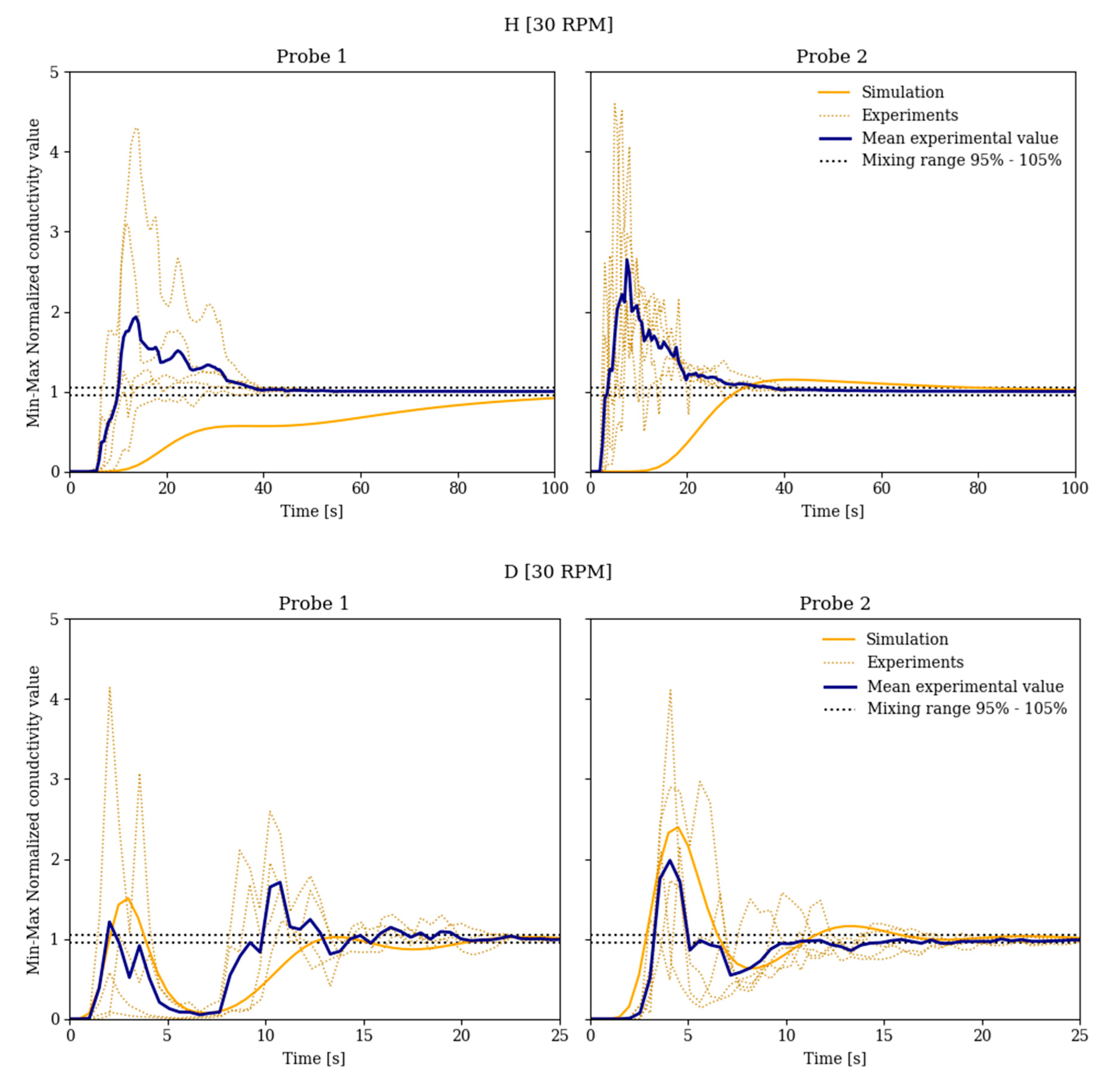
Mixing time is determined as the time when the measured concentration reaches and stays in the 95–105% range of the equilibrium concentration. Due to the shortcomings of the method used, only local concentration and subsequently local mixing times were determined experimentally. True global mixing time was only simulated and compared to local experimental and simulated mixing times. All concentrations were normalized for a fair comparison.

$$c_{norm}=\frac{c_t-c_0}{c_{eq}-c_0}$$

$c_{norm}$ presents the normalized concentration, $c_t$ presents the concentration at t, $c_0$ at $t_0$ and $c_{eq}$ presents the equilibrium concentration.

From Figure 1 and Figure 2 it can be seen that the concentration is location dependent. Differences in concentration profiles between parallel experiments are due to the unsteady nature of turbulent flow and small variations during tracer injections. As can be seen in Figure 1 and Figure 2 the average experimental and simulation concentration profiles can be in very good agreement. It can be noticed how the tracer passes the probe for the first time, which can be seen as high conductivity (concentration) peak, and also the second pass once around the vessel as the second peak. After approximately two passes, homogenization is achieved. The two probes (Probe 1 and Probe 2) were positioned on each side of the mixer. In the figures, three experiments are presented as well as the mean experimental conductivity, which is compared to the simulation.

The differences arise due to experimental variations, most importantly in unideal tracer injection. During the injections of a tracer solution, a jet formed that penetrated the liquid surface. The shape of the jet was approximated by a submerged sphere to compensate for a jet formation.

Due to the reasons explained above, more noticeable differences arise between other experimental and simulated results. As expected, global simulation mixing time is always higher than local simulation mixing times indicating that our probes are unable to determine the global mixing time. Comparing experimental local mixing times and simulated global mixing times our simulation model often underestimated mixing times. Based on similar studies that conducted experimental measurements of mixing times, we determined that there were differences between the parallel measurements of conductivity.

In experiment F the volume was 1.5 L and vessel did not have baffles. The approximate homogenization time at 30 rpm was 20 s (Figure 1, upper graphs). Baffles were introduced in experiment H, while the volume was the same, in which case the homogenization time was significantly longer, approximately 40 s (Figure 2, upper graphs). Under similar conditions, but by using a lower volume of 1 L in experiment D, the homogenization time was again reduced to approximately 20 s (Figure 2, lower graphs).

Variations were due to various causes, such as tracer volume, mixer flow properties or the tracer compound addition method [25]. The response of the conductivity probe was also simulated by computational fluid dynamics. The simulated response on the probes among the smallest tracer proportions was negligible. More noticeable changes were observed only at the largest amount of tracer compound used. Based on the collected data, we decided to use 0.1% of the tracer compound, as increasing the tracer amount does not significantly reduce the variation between parallel experiments. The flow is also disturbed to a lesser extent with the injection of a smaller amount of fluid.

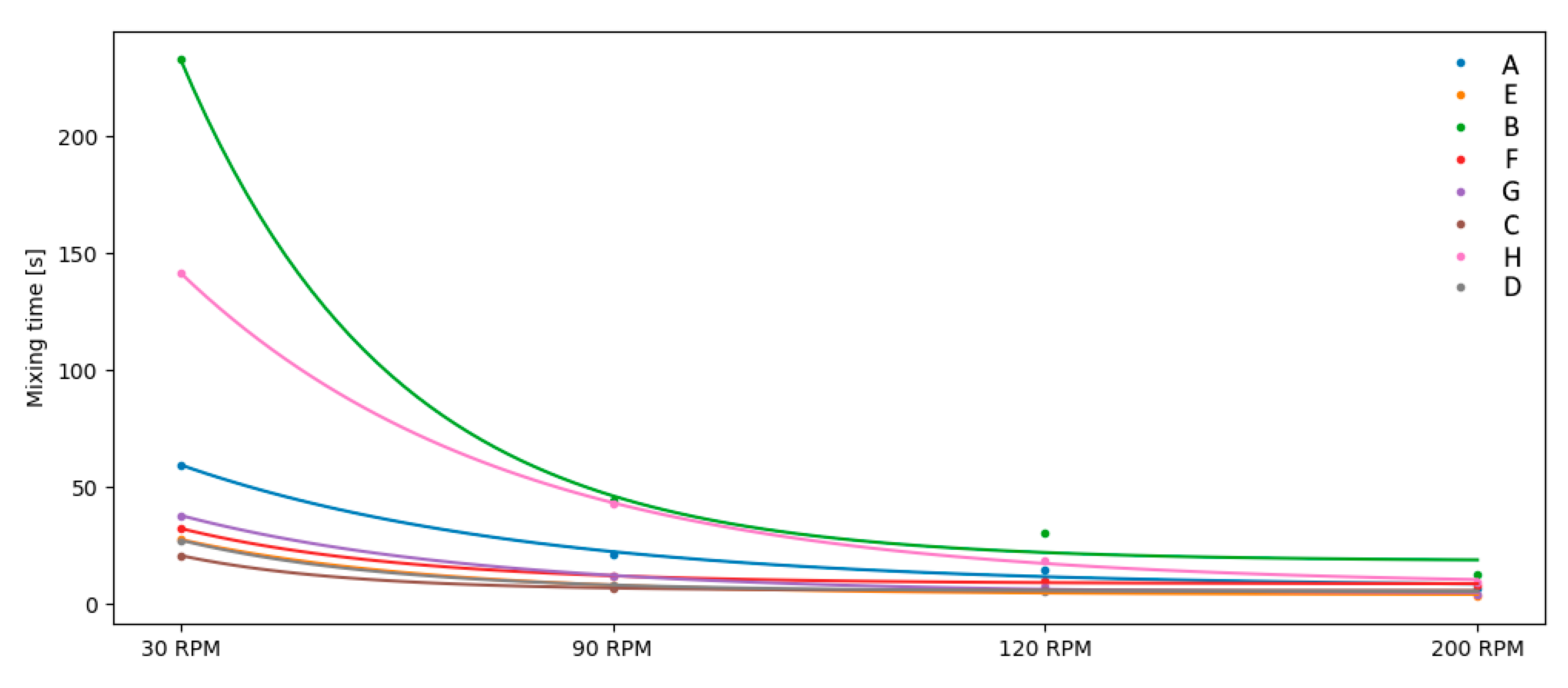
Figure 3 presents mixing times compared to different mixing speeds. As expected, the mixing time is decreased with higher mixing speed. The highest impact of mixing speed is seen between 30 and 90 rpm. From 90 to 200 rpm, the impact is mostly insignificant or negligible. In the case of 30 rpm, larger absolute differences between parallel experiments were found, which can be seen as a higher standard deviation. The differences between normalized concentration on the conductivity probes (experimentally determined and simulated) differ more when mixing speed is slow. As is commonly stated in the literature, global mixing times and local mixing times are not identical. In experiments where there is no data for the mixing time at 200 rpm, larger vortices appeared, which moved the probes for measuring conductivity in the mixing vessel, and at the same time, the liquid formed a funnel in the middle of the mixing vessel due to radial accelerations, which changed the shape of the liquid surface in the mixing vessel. Both effects have a significant impact on the reliability of the results—both on the reproducibility of the experimental results and the reliability of the simulation. From the collected data it cannot be claimed that the method used always overestimates or underestimates the mixing times, as these differ according to different experiments. An exponential decay function can be fit to simulated mixing times. The mixing time for the desired stirring speed can be extracted.

In general, mixing times in experiments with baffles and stirrers with pitched blades are longer than without the use of baffles. The mixing time when using the baffles was longer with the stirrer with pitched blades than with the stirrer with non-pitched blades. In the case of filling the mixing vessel with 1 L of liquid, the mixing time was longer in the case with no baffles, while in the case of filling with 1.5 L, a more noticeable difference occurs only at a mixing speed of 30 rpm; elsewhere the mixing times are very similar. The comparison between the stirrers themselves, i.e., without the use of baffles, also has different conclusions for different fillings. At 1.5 L filling, the mixing time is longer when using a pitched blade mixer compared to a non-pitched paddle mixer, while the result is exactly the opposite when filling with 1 L. Shorter mixing times with no baffles are unexpected, as other research has shown that baffles shorten the mixing time [26]. 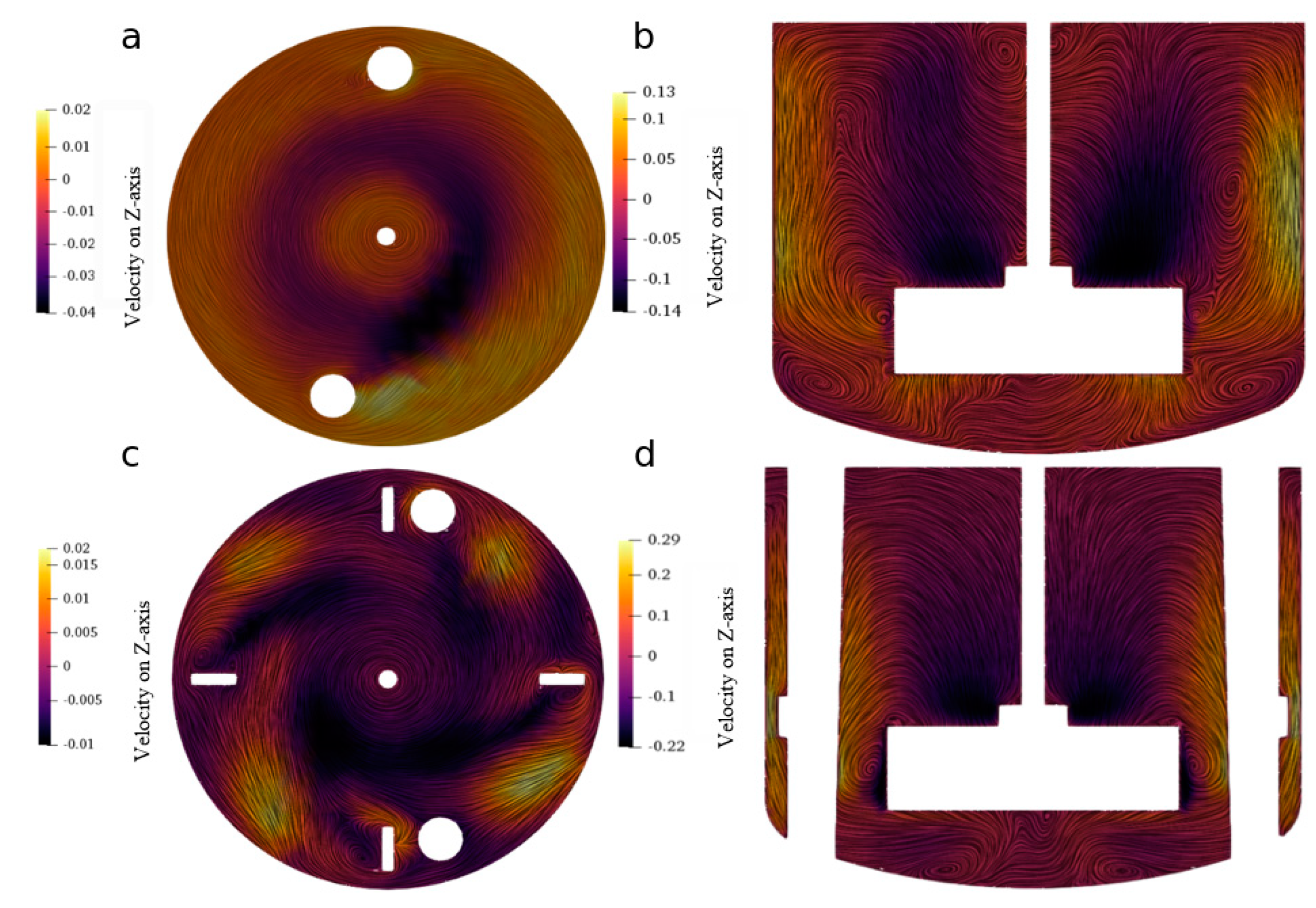Figure 4 presents the difference in velocity on the Z-axis for different experiments (C and G). It can be seen that with baffles more fluctuations on the surface occur (Figure 4c,d) compared with no baffles (Figure 4a,b). It was observed that when using baffles velocity varies dramatically between adjacent regions on the liquid surface. From experimental data it is difficult to evaluate the impact of variations during injections, as variations in measurements occur both with and without baffles, which indicates that variations are influenced to a greater extent from other phenomena mentioned beforehand.

3.2. Dissolution Results

During dissolution, sedimentation of sucrose crystals was observed. The sedimentation depended on the mixing speed and the configuration of the mixing vessel. No sedimentation occurred in the case of D3 when the stirrer speed was higher than 200 rpm. In all other experiments, a certain portion of the sucrose crystals sediment. In the experiments where sedimentation occurred, the dissolution process was divided into two parts. The first part represents the time until the suspended sucrose dissolved, while the second part represents the remaining time, i.e., from sedimentation to the end of the measurement. With increasing mixing speeds, a larger share of suspended particles was achieved. In most experiments a complete suspension was not achieved. Due to partial suspension, experimentally measured dissolution curves started flattening prematurely. After the suspended particle dissolved, the dissolution rate slowed down.

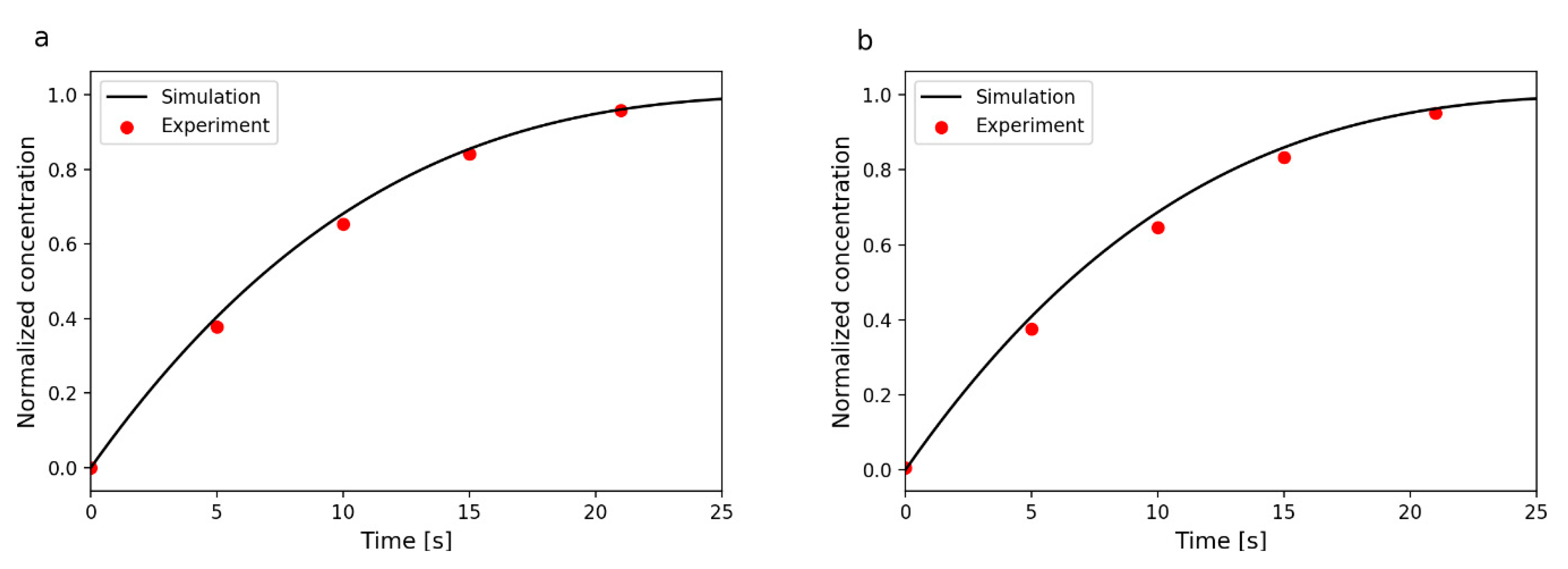
Figure 5 shows simulations for dissolution at different mixing speeds. The following can be concluded by comparing the dissolution rates. In experiment D3 (non-pitch stirrer and no baffles) the dissolution rates were the highest. At 200 rpm and 300 rpm, the rates were approximately the same, which implies that the dissolution at those mixing speeds are governed by the kinetic regime, not mass transfer. The next is experiment D2 (pitched stirrer) and no baffles. Interestingly, the configuration without baffles provides the highest dissolution rates. The baffled D1 and D4 at 200 rpm are next, so the mixing speed has more effect than the baffled or unbaffled configuration. Overall, the slowest dissolution occurred in the baffled vessels D1 and D4.

Related research has shown that the presence of baffles has a positive effect on the level of solid-phase suspended in the reactor [25]. In the case of our system, opposite results were obtained and the reason for this can be sought in the global arrangement of streamlines. Concentration at the time of sedimentation was re-standardized and thus obtained data can be compared with each other. The transfer constant obtained from the D3 300 experiment was used for all experiments. A predictive dissolution model was constructed, which was based on the substance transfer and the dissolution models described above. The time obtained from the predictive model was compared with the experimental data. The predictive model described the dissolution well; certain deviations in the form of curves were caused by slow data capture and variations in data capture by the FTIR probe. Local and global as well minimum and maximum concentrations are rapidly equalized due to strong turbulent motion caused by our choice of mixing speeds. This effect describes very similar dissolution rates for different rotational speeds. Even the lowest mixing speeds investigated are sufficient for the dissolution rates to be similar to the maximum dissolution rates. The main limitation was the amount of sucrose itself that sedimented to the bottom of the reactor. From Figure 5 it can be observed that the stirrer with non-pitch blades and baffles most effectively suspended the sucrose. The stirrer with pitched blades in combination with baffles performed the worst. From Figure 4 it can be observed that the currents in the reactor with the stirrer without blades are turned radially with a slight movement in the Z direction, on average their speed is higher. The currents in the case of using a stirrer with baffles are chaotic, they have a high speed in the region of the stirrer, but the speed decreases rapidly with a larger distance from this region. From Figure 5 it can be observed that there is a trend of decreasing dissolution time with increasing rpm. Nevertheless, there is an occasional deviation in mentioned trend. The deviation is due to the chosen model for predicting dissolution and performing the experiment itself. Due to the longer data capture on the FTIR probe, the data was filtered with a Savitsky–Golay filter, which smoothed the curve of the experimental data and thus made it possible to determine the experimental dissolution time. With this method some uncertainty was introduced, due to interpolation of the results. Given the narrow range of mixing times, therefore, even minor uncertainties can affect the trend. The rest of the error occurred due to the selected prediction method. The input data used in the predictive model—ε is inhomogeneously distributed in the mixing vessel. Only the average value of ε was used for mass transfer coefficient estimation. Even the particle distribution and particle shape itself is not completely homogeneous, which also has an impact on the mass transfer coefficient.

Table 3. Comparison of simulated and experimentally determined dissolution times and dissipation rates of turbulent kinetic energy.

Case	ε$(\frac{{\mathbf{m}}^2}{{\mathbf{s}}^3})$	Dissolution Time (Simulation) (s)	Dissolution Time (Experiment) (s)
D4 (120 rpm)	0.0238	20.00	21.15
D1 (120 rpm)	0.0124	20.30	20.56
D3 (120 rpm)	0.0107	20.40	20.90
D2 (120 rpm)	0.00868	20.50	20.84
D4 (150 rpm)	0.0452	19.70	19.89
D1 (150 rpm)	0.0275	19.90	19.84
D3 (150 rpm)	0.0262	19.90	20.99
D2 (150 rpm)	0.0157	20.20	20.56
D4 (200 rpm)	0.101	19.40	19.79
D1 (200 rpm)	0.0751	19.50	19.79
D3 (200 rpm)	0.0433	19.70	19.86
D2 (200 rpm)	0.0334	19.80	19.43
D3 (300 rpm)	0.139	19.30	19.50

presents the results for dissolution experiments and Figure 6 presents the experimental and simulated dissolution process.

The smallest difference between the experimentally determined dissolution time and the simulated dissolution time was observed for a configuration with a pitch blade stirrer and baffles. When using a stirrer without pitched blades the difference was higher.

From the simulation data, in most cases, a faster transfer of substances is observed with the use of baffles, regardless of the type of stirrer used. From experimental data, however, this claim is difficult to confirm or refute. The results themselves follow directly from the dissipation of turbulent kinetic energy (Table 3), so the relative dissolution rates can be extrapolated from these data. As already mentioned, the values of the average flow were well captured by simulations, while turbulent properties are more difficult to accurately describe due to their variable nature.

The inhomogeneity of energy dissipation is another aspect that can explain the differences between simulations and experiments. Normalization of the concentration to the concentration value at the time when suspended sucrose dissolved, affects the differences between simulations and experiments. Even though normalization was performed, the settled sucrose was still slowly dissolving into the liquid in the stirrer vessel. Sucrose at the bottom of the vessel was exposed to lower turbulence motion throughout the experiment. In the end, the estimated coefficient of mass transfer also slightly deviated, due to the dissolution of the sediment sucrose, which was neglected during normalization. Studies have also shown an association between the concentration of the suspended solid phase in the liquid and the mass transfer coefficient [25]. This effect can also have a limited effect on the mass transfer coefficient, which was not taken into account in presented model. To validate the model for use in scale up or scale down, it would be necessary to carry out experiments in even larger or smaller mixing vessels.

3.3. Flow Description

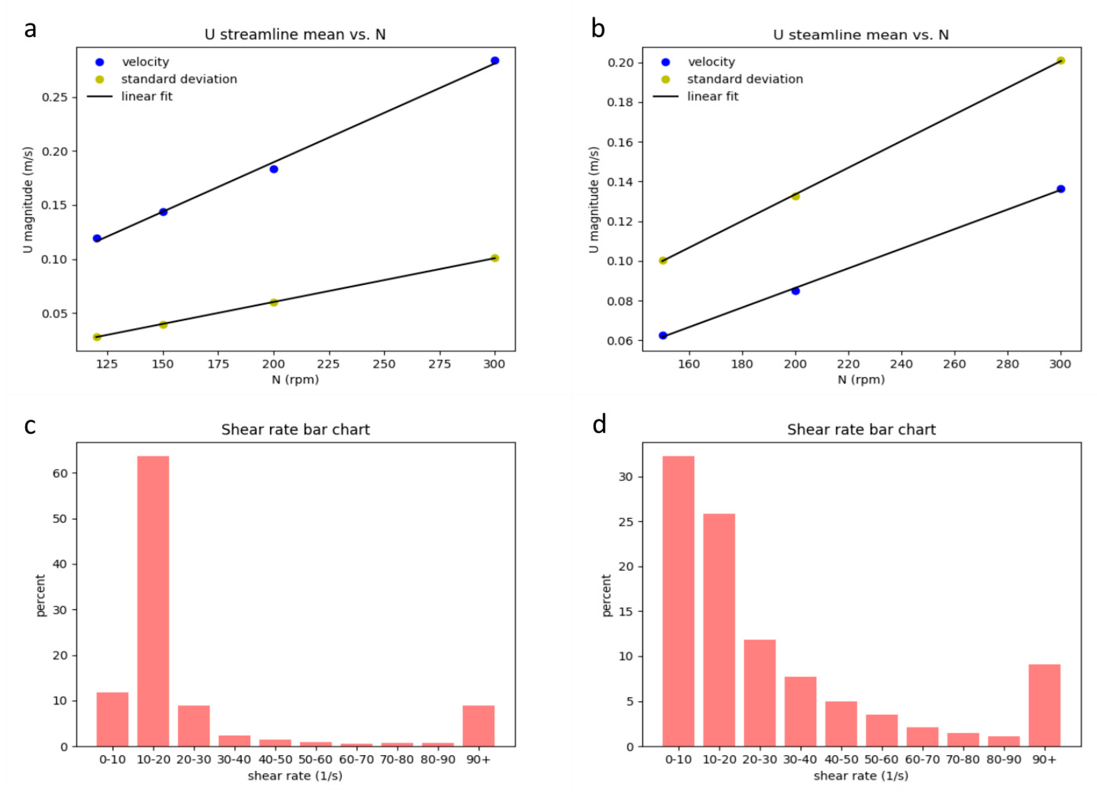
A more elaborate view of the flow dynamics in the mixing vessel can be extracted from shear rate and velocity data. A total of 200 random streamlines were extracted from each simulation. Velocity values were integrated over the streamlines and averaged to obtain the mean velocities and standard deviations from the average values for the range of speed rates simulated. This chemical reactor or mixing vessel fingerprinting method was presented in Pohar et al. [21]. Differences between experiments with or without baffles were observed. The average velocity was lower when baffles were used due to the flow being deflected by the baffles. Consequently, standard deviation increases by a factor of approximately two. On Figure 7 the top left figure presents typical unbaffled results. The mean velocity shows a linear relationship with the mixing speed (blue markers), and the standard deviations are much lower (yellow markers), due to the mostly circular motion of the fluid. On the top right figure, the baffled results show a much higher standard deviation, which surpasses the mean velocities. The differences in Figure 7 a and b, obtained by the fingerprinting procedure, give a unique representation of the fluid flow, and can be used to identify the main fluid flow characteristics such as mostly homogeneous circular flow (a) or flow with high velocity gradients (b) (in this specific case).

Similarly, the shear rate histogram, which is presented in Figure 7, is broader when using baffles, indicating that flow velocity fluctuates more from point to point. Both findings indicate a broader range of velocities and higher shear in the reactor. The higher overall shear rate due to flow irregularities could prove problematic for bioreactors which cultivate cell organisms.

The power number for a similar system was found in reference [27]. It was a pitched four-blade turbine with pitch angle α = 45°, and with the ratio of the diameter of the vessel to the diameter of the stirrer D/d = 3. The power number in the system was 1.29. In this work, the baffled 1-L system with the pitched blade was the most similar apart from the D/d, which was lower, having a value of 1.85. The power number obtained was consequently higher at the value of 1.65.

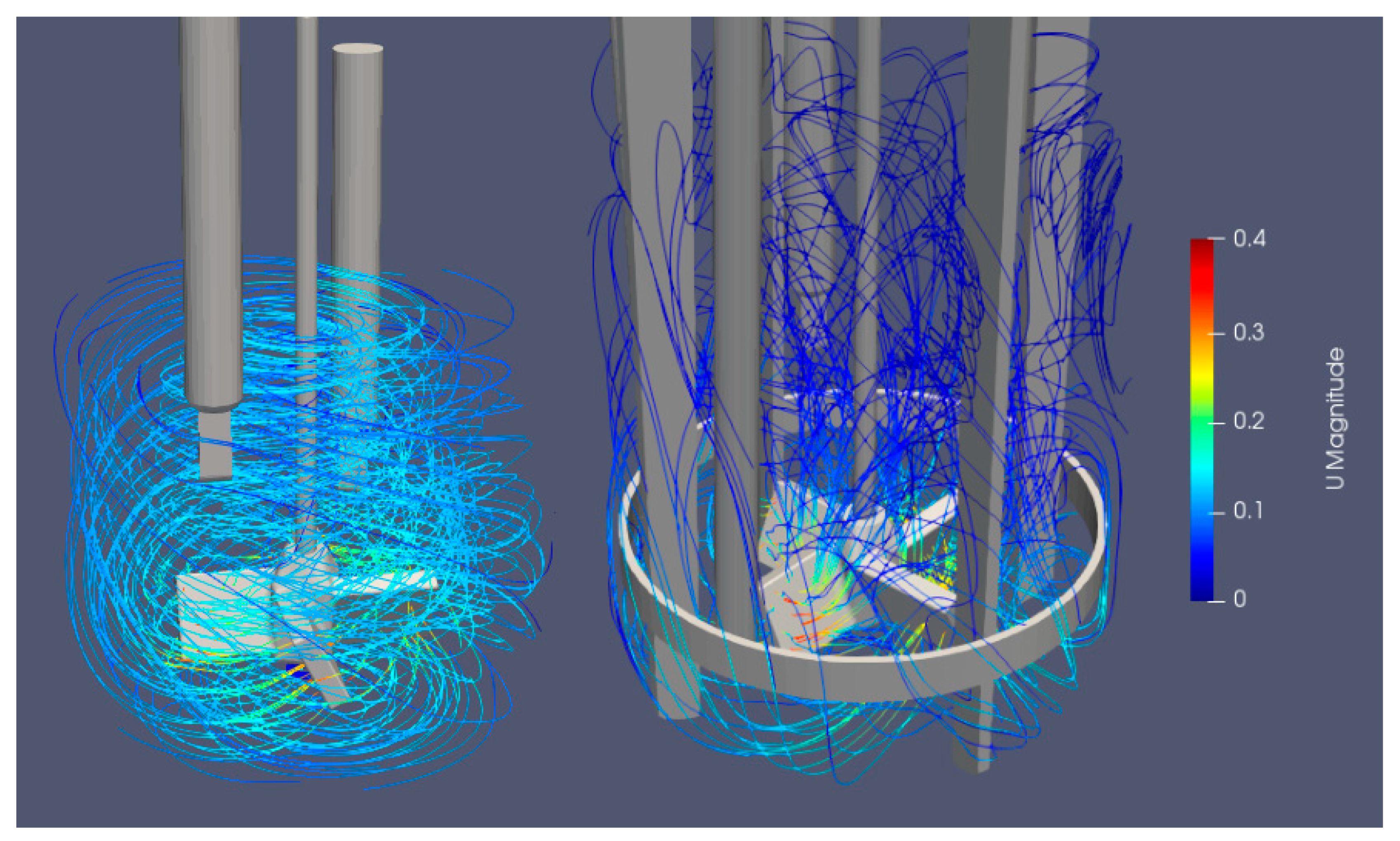
Figure 8 presents a comparison of streamlines and flow under the stirrer. The difference in flow parameters and direction is noticed. With a pitched blade, there is less liquid movement under the stirrer which is a probable reason for a larger share of unsuspended particles at the bottom of the vessel, as a slower flow is unable to suspend the particles. A similar but more pronounced effect was noticed when using baffles. The main characteristic of unbaffled mixing is a mainly circulatory mixing around the vessel, which usually causes poor mixing performance. When using baffles, a complete suspension of all sucrose particles was impossible with the mixing velocities used. By using baffles, the circulatory motion of the flow is hindered, so that it is directed also in the axial direction.

4. Conclusions

CFD is one of the methods whose industrial applicability has increased tremendously in recent years with the advent of more powerful computers. In this study, evaluation and comparison of simulations results and experiments were performed. It was found that the results of simulations for the dissolution time in the mixing vessel at the laboratory level are similar to the experimentally determined dissolution times. In comparison with other studies that concluded that baffles have a positive effect on the dissolution rate and the proportion of suspended solid phase, it was found that this is not the case in the presented manuscript and only a precise 3D model can provide the necessary information regarding the flow distribution and the mentioned mixing characteristics.

The results of this work show that: 1. CFD is a necessary tool for the evaluation of all the hydrodynamic characteristics of a mixing vessel, due to the complex three-dimensional geometries involved. For instance, using baffles would in theory produce more axial flow and should provide a shorter time for homogenization, but it was shown that this is not necessarily the case. 2. A very good agreement was found between the experimental and simulated tracer tests, which correctly predicted the tracer presence also at the second passing around the vessel to the probe. This also means that homogenization times can be accurately simulated. 3. The fingerprinting method gives a very informative description of the fluid flow inside a mixing vessel, considering the otherwise complex 3D fluid flow profiles (see Figure 7 and the discussion).