Article

Mathematical Modeling of the Production of Elastomers by Emulsion Polymerization in Trains of Continuous Reactors

by
Enrique Saldívar-Guerra
1,*,
Ramiro Infante-Martínez
1 and
José María Islas-Manzur
2
1
Centro de Investigación en Química Aplicada, Blvd. Enrique Reyna 140, Saltillo Coahuila CP 25294, Mexico
2
Dynasol Group, Planta Emulsión, Km 13.5 Carretera Tampico-Mante Int. A, Altamira, Tamaulipas CP 89608, Mexico
*
Author to whom correspondence should be addressed.
Processes 2020, 8(11), 1508; https://doi.org/10.3390/pr8111508
Submission received: 12 October 2020 / Revised: 8 November 2020 / Accepted: 13 November 2020 / Published: 20 November 2020
(This article belongs to the Special Issue Modeling and Simulation of Polymerization Processes)

Abstract

:
A mechanistic model is proposed to describe the emulsion polymerization processes for the production of styrene–butadiene rubber (SBR) and acrylonitrile–butadiene rubber (NBR) elastomers in trains of continuous stirred tank reactors (CSTRs). A single model was used to describe both processes by choosing the proper physicochemical parameters of each system. Most of these parameters were taken from literature sources or estimated a priori; only one parameter (the entry rate coefficient) was used as an adjustable value to reproduce the kinetics (mainly conversion), and another parameter (the transfer to polymer rate coefficient) was used to fit the molecular weight distribution (MWD) experimental values from plant data. A 0-1-2 model for the number of particles and for the moments of the MWD was used to represent with more fidelity the compartmentalization effects. The model was based on approaches used in previous emulsion polymerization models published in the literature, with the premise of reaching a compromise between the level of detail, complexity, and practical value. The model outputs along the reactor train included conversion, remaining monomer composition, instantaneous and accumulated copolymer composition, the number of latex particles and particle diameter, polymerization rate, the average number of radicals per particle, average molecular weights, and the number of branches per chain.

1. Introduction

Two of the most important rubber products (copolymers) from the economical point of view—styrene–butadiene rubber (SBR) and acrylonitrile–butadiene rubber or nitrile rubber (NBR)—are produced via emulsion polymerization, mainly via the continuous cold process (5–15 °C) in trains of continuous stirred tank reactors (CSTRs). Some types of styrene–butadiene copolymer rubbers can also be produced via living anionic polymerization in solution, with a better control of the composition microstructure along the polymer chain, but the subject of this paper is the random copolymer produced via radical polymerization in emulsion. The world production of SBR was estimated to be around 8.3 × 10⁶ ton/year in 2020 (based on [1]), and that of NBR was estimated to be 1.56 × 10⁶ ton/year by 2023 [2], together representing roughly 3% of the total world polymer production (assuming a total world production of 300 × 106 ton/year).
The main use of SBR is in tires and automotive applications, while NBR is used in seals, gaskets, hoses, etc., where chemical resistance, higher strength, and lower gas permeability are needed.
As mentioned above, a large portion of these copolymers is produced worldwide via continuous cold processes that, due to the lower temperatures used, avoid undesired crosslinking during polymerization. The processes for the production of SBR and NBR have many similarities, basically differing in the formulation of the emulsion components fed to the process. Both processes are performed by free-radical emulsion polymerization in a train of CSTRs at low temperatures, and they use a redox system of initiators to maintain a flux of radicals at these low temperatures. Additionally, they both are designed to reach maximum monomer conversions between 70 and 75% to avoid crosslinking due to branching reactions and to limit the composition drift. Side streams of the monomer that are consumed faster can also be included in the process to correct the composition drift in both the SBR and the NBR processes.
Concerning the cold SBR process, early models were published by the Hamielec and MacGregor group in the 1980s. Both steady-state (Kanetakis et al. [3]) and dynamic models (Broadhead et al. [4] and Penlidis et al. [5]) were presented, capable of calculating the monomer conversion, the copolymer composition, the molecular weight averages, and the long-chain branching frequency, as well as the particle size distribution (PSD), in each reactor. In the steady-state model [3], the PSD was calculated based on the known residence time distribution of a CSTR using a convolution integral to estimate the PSD in reactors downstream of the train. Only micellar nucleation was included, considering radical entry competition between micelles and already formed particles (Smith–Ewart theory); Smith–Ewart case II kinetics were assumed with 0.5 as the average number of radicals per particle ( n ˜ ) [6]. The molecular weight averages were calculated by using steady-state expressions derived by applying the method of moments. The dynamic model [4,5] had similar bases to the steady-state one, although it contains some differences in certain respects. Naturally, ordinary differential equations (ODEs) for the components of the redox initiation system, monomers, and converted monomers, surfactant, number of particles, and molecular weight distribution (MWD) moments per reactor were explicitly included. The treatment of the MWD equations was made by using the pseudo-homopolymer approach [7] (also known as the pseudo-kinetic [8] or apparent rate constants [9] methods). The evolution of the PSD was calculated in an approximated way via the discretization of the population by particle age (generations) and the use of several simplifying assumptions. In this way, only one differential equation was solved for the volume growth of a particle of the first generation, and this information was used to estimate the growth of the particles of any other generation. Interestingly, this model included the energy balances of the reactor and the cooling jacket, as well as an equation for a temperature controller. Smith–Ewart case II kinetics were also used in this model during the nucleation period and at low conversions, while at higher conversions, the extended fraction solution of the Smith–Ewart recurrence equation, proposed by Ugelstad et al. [10], was utilized to estimate n ˜ . These models were used in several applications: to determine operation policies aimed at improving the productivity of the reactor train or the quality of the SBR produced, to manipulate the PSD, to enhance the operation stability (avoiding sustained oscillations for example), and to design start-up procedures to minimize the quantity of the off-spec product [4,5]; the dynamic model adapted for semibatch operation was later used to design midcourse correction policies for the control of molecular weight and cross-linking density in semibatch SBR reactors [11].
Years later, Gugliotta et al. [12] published a model based on the Broadhead et al. model with added detail in some respects. The main differences in Guggliota et al. model with respect to [4] were:
-
The effect of impurities in the process was included.
-
The PSD was modeled by using a population balance approach for the continuous distribution N(v,t)dv, which represents the number of particles having a volume between v and v + dv at time t, resulting in a partial differential equation (PDE). This equation was approximately solved by discretizing the v domain into small subdomains ∆v and converting the PDE into a set of ODEs.
-
The monomer partitioning among phases was calculated by using the Flory–Huggins theory [13] extended to emulsion systems by Morton et al. [14] to include the effect of the interfacial energy between particles and the continuous aqueous phase.
-
The possibility of considering side streams fed to reactors along the CSTR train was included.
Similarly to the Broadhead et al. model [4], the Gugliotta et al. model [12] was applied to design policies for increasing production and transient optimization [15,16,17]. More recently, it was also used for the calibration of a soft sensor for the monitoring and control of an SBR production process using seven CSTRs in series. The model replaced actual plant data by simulating the operation of the process in an extended variable space [18].
Zubov et al. presented a detailed dynamic model for the SBR process in a train of CSTRs based on population balances and the method of moments for the description of the MWD, besides mass balances for other species [19]. Several non-conventional features are used in the model. Interestingly, they use an empirical relation for the average number of radicals in particles ( n ˜ ) as a function of the initiator concentration; as a consequence, no radical entry or radical desorption terms are used. Additionally, the transport of the monomer from the droplets to the particles is modeled by using mass transfer terms, where the concentration gradients are calculated using partition coefficients for the estimation of the equilibrium concentrations. The model is validated with industrial data for conversion, molecular weight, and Mooney viscosity for the steady-state and transient case, and its usefulness is illustrated by its application to generating a grade transition procedure to minimize the production of off-spec product. More recently, Mustafina et al. developed a rather simple model to describe the copolymer composition and other characteristics of SBR, and they used it to fit the corresponding kinetic parameters to represent intrinsic viscosity, conversion, and molecular weight data [20]. Apparently, the used data came from a train of CSTRs, but a batch model was implemented to approximately represent the process. The used MWD model was too simple and did not take branching reactions into account.
Regarding the NBR case, the apparently first mathematical models for batch and semibatch industrial processes were published, almost simultaneously, by Dubé et al. [21] and by Vega et al. [22]. The Dubé et al. model was built to represent batch and semibatch reactors while considering redox initiation, the thermodynamic partitioning of monomers among phases using the partition coefficients model, and the pseudo-kinetic rate constants method for the copolymerization kinetics; n ˜ was calculated by using the Ugelstad [10] expression. The model was capable of predicting conversion, the number of particles per L of water Np, the rate of polymerization Rp, the copolymer composition, the number and weight average molecular weights Mn and Mw (by the method of moments), the branching averages, and the average particle diameter Dp.
The model of Vega et al. [22] was also written for batch and semibatch reactors, and it was an extension of the previous model built by this group for the SBR process [12] (which was itself based on the Broadhead et al. model), with some modifications to capture the mechanistic features generated by the presence of the more water-soluble acrylonitrile (AN) monomer. The modifications of the model included the polymerization of AN in the aqueous phase, radical desorption, and homogeneous nucleation. However, some of these modifications were only applied to the polymerization rate but not to the MWD calculations, making these two parts of the model somewhat inconsistent. The latter model was further extended in [23] to describe in more detail the bivariate chain length and branching distribution in the batch case. It was also used to simulate plant data for testing an open-loop estimator based on calorimetric measurements to monitor NBR properties in a semibatch process [24]. Notice that none of the previous cited works addressed continuous NBR production processes; it was only in the works of Minari et al. [25,26] that the Vega et al. model was extended to the case of a train of CSTRs for NBR production to study the effect of intermediate feed streams of chain transfer agents (CTAs) and AN on the polymer quality [25] and to reduce transients during grade transitions [26]. More recently, the model of Vega et al. was used to evaluate a closed-loop control strategy to produce the NBR of uniform copolymer composition in a semibatch reactor [27].
Another model for NBR production in a train of CSTRs (also used for batch and semibatch operations) was proposed by Washington et al. [28,29]. This model was based on that of Dubé et al. [21] with many similarities: redox initiation, the partitioning of monomers described by partition coefficients, the use of pseudo-kinetic rate constants for the reaction kinetics, and the calculation of n ˜ by using the extended fraction expression [10]. It also used an average particle size and consisted of differential equations (dynamic model). As in the case of other models for continuous reactors, it was used to study start-up procedures and the control of polymer properties (copolymer composition, molecular weight, and particle size).
More recently, the Washington et al. model was used to study, in more detail, the effect of the monomer partitioning model, the radical desorption, and the monomer soluble impurities of several polymer properties in the batch and the CSTR train case. [30] The model was also applied to study dynamic aspects of a train of eight CSTRs and the effect of different operation policies on the off-spec material produced during transient operation. [31] Scott et al. also used this model to demonstrate the application of the Bayesian experimental design technique to maximize the information that can be experimentally obtained for an NBR process carried out in a train of CSTRs [32].
In summary, there are few models for trains of CSTRs for the production of SBR ([3,4,12,19,20]) and NBR ([25,26,29]). Many of the models ([12,25,26]) stemmed from the same model of Broadhead et al. [4] with some adaptations, and others ([3,29]) are not very different either in terms of assumptions and structure.
Given the similarities of the SBR and NBR processes, it was the goal of this work to develop and present a single model that is flexible enough to represent both processes with relatively small variations and to demonstrate that the same mathematical structure could be applied with minor adjustments to both processes. Some previous models have addressed only one of the two polymerization systems at a time (not necessarily for the continuous process but for batch or semibatch modes), although, in some cases, they used essentially the same model with adaptations. We believe that it is instructive to treat the two processes with the same model simultaneously in order to emphasize their similar underlying structures. Other goals of this work were to introduce improvements in some key aspects of the models (to be specified below) and to reach a good balance between the level of detail, the ease of implementation, and the predictive power of the model. To do this, a different model is proposed that is intended to study the effect of the configuration of the CSTR’s train in the production (rate and quality) of both SBR and NBR elastomers. Configuration refers to the number of reactors in the train (in the range of 7–16), as well as the possible presence and position (reactor number) of side feed streams of one of the monomers or CTAs in the reactor train.
The goal of the study was to compare steady-state operations; nonetheless, a dynamic model was written in the form of ordinary differential equations (ODEs) since, in our experience, the numerical solution of this kind of system is more robust than that of the corresponding steady-state non-linear algebraic equation system. This selection was based on the experience of many years of our group working on the mathematical modeling of industrial emulsion polymerization processes.

2. Mathematical Model

In this section, the different components of the used mathematical model are presented and briefly discussed. Since some of these components were taken or adapted from existing models—only the main features of them are provided, and their details can be found in the given references and in the Supplementary Materials (SM).
The philosophy of the present work during the definition of the different components of the model was to use only the level of complexity deemed necessary to have a reliable description of each of the involved phenomena. In some cases, as in the calculation of n ˜ , which was based on a 0-1-2 particle model adapted from one by Vale and McKenna [33], this choice resulted in an increased level of detail compared with previous models. Additionally, the present model uses a more detailed calculation of the leading moments (0–2) of the MWD which, for consistency with the particle model, were also calculated using a 0-1-2 model based on a subset of the population balance model of Saldívar et al. [9] The model is not just a collection of existing pieces from other models, but the equations were re-derived and/or adapted as needed. In other cases, our choice was a simpler model than those in other works; this was the case, for example, of the monomer partitioning model, which is quite simple but still effective. A more detailed discussion of these differences is provided in the specific sections of the paper.
The used kinetic scheme is given in Table 1. Notice that the medium part of the table shows, in detail, the terminal model on which the pseudo-homopolymer approach was based (for propagation and chain transfer to monomers and CTAs). Diffusion-controlled termination using a single coefficient was used. The lower part of the table shows the kinetics in the pseudo-homopolymer form, which is particularly useful for the MWD (moments) calculations. Notice that the internal and terminal double bond reactions only occur on the butadiene units of the dead polymer, and this is reflected in the multiplication of the corresponding rate constant by F 1 , m o c , which is the accumulated molar fraction of butadiene in the polymer.
The symbols used in Table 1 for the aqueous phase are: I w , initiator; Y 1 r and Y 1 o , reducing agents in the reduced and oxidized states, respectively; Y 2 ,   secondary reducing agent; R w , primary radicals in the aqueous phase; P w , polymeric radicals in the aqueous phase; and D w , the dead polymer in the aqueous phase. For the particle phase, the nomenclature is: P i , polymeric radicals of type i terminal unit; M j , type j monomer; D , the dead polymer; P r and D r , length (r) of live and dead polymers, respectively; M ,   total monomer ( M = M 1 + M 2 ); and T ,   chain-transfer agent. Notice that P r = P 1 r + P 2 r , where P i r are r-length polymeric radicals of type i (i = 1,2).
The following equations are valid for any reactor in the train, except where noted.

2.1. Monomer Mass Balances

The remaining mass of monomer M i m (i = 1,2)
d M i m   d t =   F i n w M i ,   i n M i m   F o u t M T   F i , m a R p V w M w i + F r i , M i
Monomer bound in the polymer chain H i m (i = 1,2)
d H i m   d t =   F i n w H i ,   i n H i m   F o u t M T + F i , m a R p V w M w i
where M w i is the molecular weight of monomer i; w s ,   i n is the inlet mass fraction of species s entering the reactor; F i , m a is the mass fraction of monomer i instantaneously formed in the reactor according to the Mayo–Lewis equation in mass form; F i n and F o u t are the inlet and outlet total mass flows entering and exiting the reactor, respectively; M T is the total mass in the reactor; R p is the reaction rate, mol/(L s); and V w is the water volume in the reactor. Notice that the reaction rate is defined per liter of the aqueous phase. F r i , M i are side feed streams (mass flow) of monomer i to reactor ri.
The Mayo–Lewis equation in molar units is:
F i , m o = r 1 f 1 2 + f 1 f 2   r 1 f 1 2 + 2 f 1 f 2 + r 2 f 2 2  
where F i , m o (i = 1,2) is the mole fraction of i-monomer units instantaneously incorporated in the copolymer; f1 (i = 1,2) is the mole fraction of monomer i remaining in the reaction site; and ri (i = 1,2) comprises the reactivity ratios of the copolymer system. The two forms (molar and mass) of the equation are related by a simple function fM that converts the molar fraction into the mass fraction:
F i , m a = f M F i , m o ,   f 1 ,   M w i
where M w i is the molecular weight of monomer i (i = 1,2).
Notice that for practical reasons, mass, instead of molar units, is used for some of the balances, since the recipes are handled on a mass basis in industrial practice.

2.2. Rate of Polymerization

The polymerization rate can be calculated with the classical expression for emulsion polymerization:
R p = k ¯ p n ¯ M p N p N a    
where [ M p ] is the monomer concentration in particles, mol/L; n ¯ is the average number of radicals per particle; N A is the Avogadro number, mol−1; N p is the number of particles per L of water, L−1; and k ¯ p is the apparent rate constant for propagation, L (mol s)−1, calculated as:
k p ¯ = i = 1 2 j = 1 2 p i j k p i j  
where p i is the probability of type i radical in particle (i = 1,2) and i is the mole fraction of monomer i in particle (i = 1,2). The probabilities p i can be calculated as shown in [34].

2.3. Population Balance Equations for Particles and Calculation of R p and n ¯

Defining F n , r i as the number of particles with n radicals (n = 0,1,2) per liter of water, L−1, in the reactor ri in the train, population balance equations (PBEs) based on those postulated by Vale and McKenna [33] for a 0-1-2 system can be obtained. These equations are different from those of Vale and McKenna in two aspects: they do not consider the full-size distribution (partial derivatives with respect to size) but an average particle size instead that can increase with time and/or reactor. Another difference is that these equations include the inflow and outflow terms not present in the batch model of Vale and McKenna:
  d V w F 0 , r i d t = ρ F 0 , r i + k d e s F 1 , r i + 2 k t υ F 2 , r i + Q i n , r i F 0 , r i 1 Q o u t , r i F 0 , r i
  d V w F 1 , r i d t = ρ F 0 , r i ρ + k d e s F 1 , r i + ρ + 2 k d e s F 2 , r i + ρ m i c M i c + Q i n , r i F 1 , r i 1 Q o u t , r i F 1 , r i
  d V w F 2 , r i d t = ρ F 1 , r i ( ρ + 2 k d e s + 2 k t υ ) F 2 , r i + Q i n , r i F 2 , r i 1 Q o u t , r F 2 , r i
where ρ , k d e s , and k t are the radical entry, radical exit, and termination rate coefficients, respectively (see details and units below); v is the volume of an average particle, L; M i c is the micelle concentration L−1; Q i n , r i and Q o u t , r i are the total in and out volumetric flows to and from reactor ri, respectively; and k t = k t ¯ N A   . Notice that the radical entry and exit coefficients are particle size-dependent as detailed below. The micellar nucleation mechanism is included in Equation (8); in general, the radicals in the aqueous phase may enter micelles or particles in a competitive way.
A dimensionless version of these equations, used for the numerical solution of the model, can be found in the Supplementary Materials.
From the solution of Equations (7)–(9) it is possible to calculate n ¯ and N p   from the following expressions:
n ¯ = n = 0 2 n F n n = 0 2 F n    
N p = n = 0 2 F n    

2.4. Radical Entry and Exit Coefficients

The used specific expressions were taken from [9], but they were based on concepts previously proposed and generally accepted [35,36,37]. See the Supplementary Materials for specific details; Supplementary Material Equations (S1a)–(S1o).

2.5. Mass Balances of Species

In all the balance equations, w S p , i n represents the mass fraction of species S p in the reactor feed and M S p   is the molecular weight of S p (except for M T   that is total mass in the reactor). Differential equations representing the balances are written in molar units, except where noted. They are written for the initiator I w , reducing agents Y 1 and Y 2 , surfactant S , and chain transfer agent T r , and they are summarized below. More details on the assumptions and derivation of theses equations are included in the Supplementary Materials.
Initiator I w :
d I w d t = k d 1 Y 1 r   I w / V w   + F i n w I ,   i n   M I I w   F o u t M T
Reducing agents Y 1 and Y 2 :
d Y 1 d t = F i n w y 1 ,   i n M y 1 Y 1   F o u t M T
d Y 2 d t = F i n W y 2 , i n   M y 2   Y 2 F o u t M T k d 2 Y 1 o Y 2 / V w
For further details on the use of these equations, see Supplementary Material Equations (S1a–S1r) in the Supplementary Materials.
Surfactant S:
d S d t =   F i n w s , i n M s   F o u t S M T
The surfactant balance is connected and solved simultaneously with the corresponding adsorption equilibrium (Langmuir isotherm) described by the Supplementary Material Equations (S1u)–(S1x) in the Supplementary Materials.
Given the total amount of surfactants by the mass balance, the partitioning of the surfactant adsorbed in particles ( S a ), and free in water ( S f ) can be defined; S f is given by a quadratic equation and includes the surfactant in solution and the surfactant in micelles. The micelle concentration is obtained by Equation (16) or (17):
M i c = S f / V w   S c m c N A a e m 4 π   r m 2   if   S f / V w   S c m c
M i c = 0   if   S f / V w   <   S c m c
where S c m c is the critical micelle concentration of the surfactant (mol L−1), a e m is the surface area per surfactant molecule, and r m   is the radius of a micelle.
Chain transfer agent (Tr):
d T r d t =   F i n w T r , i n M T r   F o u t T r M T k t r T T r p     n = 1 2 n F n N A   V w + F r i , T r   M T r
where F r , T r   is a side feed stream (mass flow) of CTAs to reactor ri. The partitioning equilibrium of the CTAs defines their concentration in the particles. This is based on the assumption that the component partitions between the particles and the aqueous phase according to the partition coefficient are defined as:
K T =   T r p T r w
where T r p and T r w are the concentrations of CTAs in the particle and aqueous phase, respectively.
The simultaneous solution of the mass balance and the CTA partitioning is described in detail by Supplementary Material Equations (S1y)–(S1aa) in the Supplementary Materials.
Water (in mass units):
d W d t = F i n w w 1   i n   F o u t   W M T
Differential mass balance equations were also derived for primary radicals R w and polymeric radicals P w (aqueous phase), but the quasi-steady state approximation (QSSA) was assumed for these species, resulting in a simple quadratic equation for P w :
  k t   P w 2 / V w   k m p 4 π   r 2   P w   n = 0 2 F n   k m m a m   M i c   P w +   K d e s N A   n = 0 2 F n +   k d 1 f Y 1 r   I w / V w = 0
where k m p   is an entry coefficient for radicals in particles (m/s−1); r is the radius of an average particle; k m m is the entry coefficient for radicals in micelles; a m is the total micellar surface area; and M i c (L−1) is the micelle concentration.

2.6. Monomer Partitioning

The modeling approach used here was relatively simple but still effective. Madhuranthakam and Penlidis [30] concluded that the use of different models for monomer partitioning (e.g., partition coefficients and models based on equations of state) does not make a significant difference in the case of the more complex NBR system in which the water solubility of AN is important. For the simpler SBR case, an equipartition approach (similar proportions of the monomers in the droplets and particle phases) equivalent to that proposed by Dougherty [38], is used. Additionally, the approach used here allows for the a priori estimation of key parameters of the partitioning model based on the known physicochemical properties of the system components. The used modeling approach was based on the simple limit conversion for saturation, x s a t , used by Gardon [39] as the conversion at which the monomer droplets disappear (end of interval 2). Up to this point, in the presence of excess monomers, the polymer particles are saturated with monomers and maintain a nearly constant concentration ( M p ).
M p is calculated differently depending on the stage (interval) of the polymerization. The decision is made based on the equivalent conversion, x , defined as:
x = P 1 m + P 2 m M 1 m +   M 2 m M 2 w + P 1 m + P 2 m
where M 2 w   stands for the mass of monomer 2 in water. This latter quantity is nearly zero for SBR, but it is significant for NBR due to the partial solubility of AN in water.
If x   x s a t (intervals 1 and 2), M p is calculated by the Equation (23). The details of how to arrive to this equation and how to calculate each of the involved quantities can be found in the Supplementary Materials Section 2, Supplementary Material Equations (S2a)–(S2c) of the Supplementary Materials.
M p =     M p s a t = M 1 / M w 1 +   M 2 / M w 2 V p
where V p is the volume of this hypothetical particle, which can be calculated assuming volume additivity:
V p = M 1 ρ 1 + M 2 ρ 2 + P 1 ρ p 1 + P 2 ρ p 2
where M w i = molecular weight of monomer i and   ρ i and ρ p i   (i = 1,2) are the densities of monomer i and homopolymer i, respectively.
If x   >   x s a t ( m a s s   c o n v e r s i o n   x , interval 3), M p is calculated assuming that all the remaining monomers, except for the possible presence of AN in the water phase (NBR case), are in the particles:
M p =     M 1 m / M w 1 +   M 2 m M 2 w m / M w 2 V p
where:
V p =   M 1 m ρ 1 + M 2 m M 2 w m ρ 2 + H 1 m ρ p 1 + H 2 m ρ p 2
and the superindex m indicates mass units.
An approximate way of estimating the amount of AN in the water phase ( M 2 w ) in the NBR case is based on a partition coefficient, defined as the ratio of mass concentrations of monomer 2 in the particles and the water phase:
χ A N =     ( M 2 m p ( M 2 m w
As shown in Supplementary Materials Section 2 (see Supplementary Material Equation (S2d)), M 2 w can be obtained by solving the following quadratic equation:
χ A N ρ 2 M 2 w 2 χ A N M 1 m ρ 1 + M 2 m ρ 2 + P 1 m ρ p 1 + P 2 m ρ p 2 + V w M 2 w + M 2 m V w =     0

2.7. Total Mass Balance

Since there might be side-feed streams of monomers and/or CTAs along the train, a total mass balance per reactor (in mass units) is necessary:
d M T , r i d t = F i n , r i F o u t , r i + F r i , t r + F r i , M 1 + F r i , M 2
where M T , r i is the total mass present in reactor r i (reactors of different volumes can be considered along the train). Notice that in previous equations, the second subindex ri was omitted when it was clear that the balances were written for any reactor in the train. The same convention is used for the total mass flows entering and leaving the reactor ( F i n , r i and F o u t , r i ,   respectively). As an approximation, it is assumed that the time derivative is zero; that is, a constant mass is maintained in each reactor. In reality, a constant volume operation is used instead (level control); nonetheless, since the density variations are relatively small, this approximation introduces little error during the transient calculations and no error when the steady-state is achieved. In this way, the total output mass flow can be explicitly calculated from Equation (29) because the other terms are known (naturally, F i n , r i = F o u t , r i 1   for ri > 1).

2.8. Molecular Weight Distribution

The quantities of two different distributions, one for the live polymer and the other for the dead polymer, are defined as follows:
N n r = number of length-r radicals in particles having n radicals, per L of water.
D n r = number of length-r inactive polymer chains radicals in particles having n radicals, per L of water.
For the assumptions and details of the derivation of the corresponding PBEs, the reader is referred to [9]. Though the derivations used here follow the general assumptions in [9], the model was adapted to comply with the 0-1-2 scheme. Some of the terms in the balances represent a shift in the classification of radicals in the presence of a given kinetic or physicochemical event.
A general balance for the live polymer r = 1 ,   2 ,   3 and n = 1 ,   2 ,   3 ,   in any reactor, where the identification of the reactor number (ri) is kept only for the inlet and outlet mass flows, is:
d   V w   N n r d t   =   k p N n r 1 [ M ] p V w k p N n r [ M ] p V w k t r M N n r [ M ] p V w +   k d e s   n   N n + 1 r k d e s   N n r n 1 K t r T N n r [ T r ] p V w + ρ N o   δ   n = 1   δ   r = 1 +   ρ m i c   M i c   δ n = 1 δ r = 1   k d e s   N n δ   r = 1 δ n = 1 + ρ   N n 1 r   ρ N n r / n +   k t r T N n [ T r ] p   V w δ r = 1 + k t r M N n [ M ] p V w δ r = 1 + k t V w 2 N A v [ n n + 1   N n + 2 r n n 1 N n r ] + ρ N 2 r 2 δ   n = 1 + k d b F 1 [ j = 1 j D n j N n r + j = 1 r j D n j N n r j ] n V w N n N A v + [ k t r p j = 1 j D n j N n r + k t r p r D n r j = 1 N n j ] n V w N n N A v + F i n , r i w w f N n r , f / ρ w N n r V w F o u t , r i M T
where δ   j = j 0 represents the Kronecker delta function, which is 1 when a given integer variable j = j 0 and is 0 elsewhere. For a dead polymer, the balance is, in principle, valid for r = 1 ,   2 ,   3 and = 0 ,   1 ,   2 ,   3 ; the resulting PBE is:
d V w D n r d t = ρ D n 1 r D n r + k d e s n + 1 D n + 1 r k d e s n D n r + V w k t r M M p N n r + V w k t r T T r p N n r + V w 2 N A v k t n + 2 n + 1 D n + 2 r V w 2 N A v k t   n n 1 D n r + k t d V w 2 N A v n + 1 N n + 2 r + k t c V w 2 N A v   n + 1 N n + 2 j = 1 r 1 N n + 2 j N n + 2 r j        + k t r p r D n r j = 1 N n j + k t r p N n r j = 1 j D n j n V w N n N A v        k d b F 1 r D n r j = 1 N n j n V w N n N A v + F i n , r i w w f D n r , f / ρ w D n r V w F o u t , r i M T
where w w f is the mass fraction of water at the inlet and P n r , f and D n r , f are the values of the distribution in the inlet stream for the live and dead polymers, respectively.
Since a 0-1-2 model was to be used, Equation (30) was applied only to n = 1,2, while Equation (31) was applied to n = 0,1,2. Then, the method of moments was applied to derive equations for the following moments:
μ K , n = r = 1 r K   n = 1 ,   2 ,   K = 0 ,   1 ,   2
λ K , n = r = 1 r K D n r   n = 0 ,   1 ,   2 ,   K = 0 ,   1 ,   2
where μ K , n   and λ K , n   are the K-th moments of the live and dead polymers, respectively, in particles having n radicals. Only the first three moments (0, 1, and 2) of both populations are needed to calculate the number- and weight-average molecular weights. The final equations for these moments, six for the live polymer (Supplementary Material Equations (S3d)–(S3i)) and nine for the dead polymer (Supplementary Material Equations (S3j)–(S3r)), are provided in the Supplementary Materials, both in their original and dimensionless versions. The modeling approach followed here involved much more detail than previous modeling efforts since a full set of moments (0–2) had to be calculated for particles with 0, 1, and 2 radicals and then added together, taking compartmentalization effects into account more faithfully.

2.9. Number of Branches

The number of branches, B, per L of water in any reactor, can be estimated simply by the following ODE:
d B V w d t = F i n w w f B f ρ w F o u t V w B M T + k t r p + k d b N A V p n = 1 2 n λ 1 , n   V w
In steady-state, this can be written as:
0 = F i n B f M T F o u t B M T + k t r p + k d b N A V p n = 1 2 n λ 1 , n    
or, equivalently:
B =   F i n B f F o u t + M T F o u t k t r p + k d b N A V p n = 1 2 n λ 1 , n  

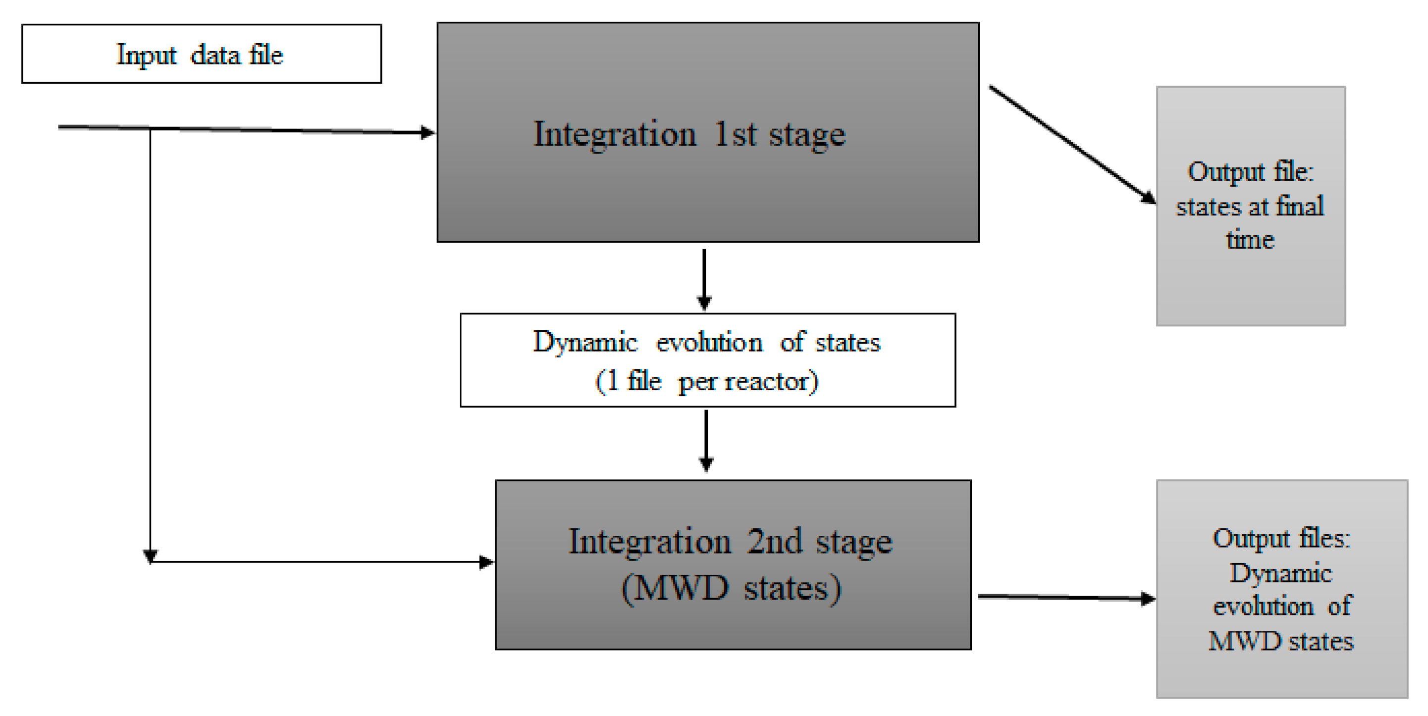
2.10. Strategy of Solution

The model described in the previous section resulted in a first set of 13 ODEs per reactor (ri) associated to the states M 1 , M 2 ,   H 1 , H 2 , S , W , T r ,   I w ,   Y 1 , Y 2 , F 0 , r i , F 1 , r i , and F 2 , r i , as well as 15 additional ODEs per reactor for the moments of live (6) and dead polymers (9) (Supplementary Material Equations (S2d)–(S2r)). Note, however, that the equations for the live polymer moments μ 0 , 1 and μ 0 , 2   did not need to be solved, since equivalent information could be obtained from the solution of Equations (8) and (9) by realizing that μ 0 ,   1 F 1 , r i and μ 0 ,   2   2 F 2 , r i . Though the number of branches B could be dynamically calculated using Equation (34), it was decided to calculate its value only at the final steady-state by using Equation (36). In summary, the model resulted in a set of 26 ODEs per reactor. A summary of the ODEs and the most important auxiliary equations, which are the set of working equations implemented in the solution code, is included in Table 2.
To reduce the stiffness of the ODE system, the QSSA was applied to the remaining 4 live polymer moments. Simple explicit algebraic expressions were obtained for these variables, reducing the effective number of ODEs per reactor to 22.
Given the relative complexity of the equations (especially those related to the MWD) and to facilitate the programming and debugging steps of the implementation of the numerical solution of the ODEs, this task was implemented in two stages. In the first stage (computer program), only the first 13 ODEs (for each reactor) were integrated by using a given set of initial conditions in all the reactors in the chain until the steady-state was reached. The set of initial conditions was designed to reach the steady-state fast; linear profiles of the species along the reactor train, according to the approximate profiles expected at the steady-state, were used as the initial conditions. The evolution of the states was recorded at regular time intervals in a file, as illustrated in Figure 1. The variables in the first set of ODEs are independent of the MWD, and, therefore, the corresponding equations could be solved first. Once the solution of this set was obtained, the set of ODEs corresponding to the MWD was numerically solved in a dynamic way in a second computer program by using the dynamic information of the states obtained from the previous integration stage. To obtain more accuracy in the second stage, linear interpolation was used as needed to obtain values of the variables in the first set at integration times between the recorded time intervals (every ~20 s). The numerical routine DDASSL (Differential-Algebraic System Solver) [40] was used in the two stages (programs) for the integration of the equations, which were coded in Fortran. DDASSL is capable of solving either a system of differential-algebraic equations or a system of pure ordinary differential equations, and, since the present system is numerically a system of ODEs (all the coupled algebraic equations are explicit), any ODE integrator for stiff equations could have been used. In this case, all the variables were declared as double-precision in Fortran, and the used numerical relative tolerance was 10−7–10−6. These numerical parameters allowed for safe and robust convergence in all cases. The execution of each stage took ~1–2 s from time zero to the achievement of the steady-state in a standard laptop, even in the case of simulations for the maximum number of implemented reactors (16 in a train). The simulated time needed to achieve the steady-state was around 2–3 times the overall residence time of the reaction in the reactor train, which is usually close to 5 h. The implemented solution strategy turned out to be efficient, robust, and relatively easy to debug.

3. Results

3.1. Parameter Values

The first problem to solve for the practical use of the developed computer programs was the selection of the physicochemical parameters of the simulated systems (SBR and NBR). Many of them were found in literature sources, but in several cases, the information was scarce or nonexistent. In the latter cases, most of the parameters were estimated a priori based on reasonable assumptions or indirect information; for example, the kinetic constants of the redox initiation system were estimated a priori based on data on the concentration of initiator at the last reactor exit. Notice though that these should not be considered adjustable parameters, since they were not fitted after comparison with the experimental data corresponding to the model outputs but estimated before the simulations were performed. A possible concern with this approach is how significant is the effect of these parameters on the final calculations and, therefore, if the error introduced with these estimations is significant. To answer this, the discussion can be better organized by classifying the prior-estimated parameters into three categories that are discussed next:
-
Kinetic parameters ( k d 1 ,   k d 1 ,   f ,   C M 1 ,   C M 2 ,   C T 1 ,   C T 2 ): These were based on independent kinetic data (e.g., the kinetic constants of the redox initiation system, as discussed above) or assumed similar to values published for chemically similar systems; therefore, it is expected that little error could be introduced through these parameters.
-
Surfactant-related parameters ( r m ,   a e m ) : These were also estimated by assuming similar values to those of chemically similar systems, which vary within relatively narrow ranges, so no significant errors are expected associated with these estimations.
-
Desorption-related coefficients ( D w T ,   D p T ,   m d ,   m d T ) : These parameters enter into the expressions of the desorption coefficient (see Supplementary Material Equations (S1h)–(S1i)) and do not have strong influence on the final responses, according to our experience.
-
Partition coefficients ( K T ,   χ A N ) : These parameters were inferred from known values of the solubilities of the respective components in water and organic media, so it is expected that the estimations used were not far from the real values. Indirect evidence of the adequacy of these estimations came from the behavior observed in the model for responses affected by these parameters, such as the copolymer composition (NBR case) and the molecular weights, which were close to experimental values.
Essentially, only one parameter was left as an adjustable value (entry rate coefficients to micelles and particles which were assumed equal, k m m = k m p ) to fit the kinetic data (mainly conversion), and a second parameter (transfer to polymer rate coefficient k t r p ) was used to fit the MWD dispersity. This was justified since the value of the last parameter is usually model-dependent, as it is quite difficult to estimate it from independent experiments; see, for example, [28]. Since both the k t r p   and the k d b affect the MWD dispersity and the number of branches B but it is practically impossible to discern their individual values based solely on the experimental values of the dispersity and B , it was decided to arbitrarily set k d b = 0 and to fit only the value of k t r p , which should then be considered as an effective value. In principle, it should be possible to measure by 13C NMR techniques the number of trifunctional and tetrafunctional branches, mainly associated with transfer to polymer (one tertiary carbon) and internal double bond (two tertiary carbons) reactions, respectively, and from these values to independently obtain a rough estimate of both kinetic coefficients; however, this fell out of the scope of the present work. Regarding propagation and termination coefficients, it is well-known that the most reliable values for these parameters are those obtained by pulse laser polymerization (PLP) (when available), and there have been some reported for these coefficients for styrene and AN (see for example [41,42] for propagation coefficients); however, it was also interesting to compare the model results with kinetic parameters that had been used before by other groups working with emulsion systems, in particular for styrene polymerization, [43] or specifically for NBR polymerization, [24,28], even though they were not determined by PLP. Both types of parameters were tested in the present model; however, for comparison with previous work, the values shown in the simulations were not necessarily obtained with PLP-determined parameters (see details in Table 3). Nonetheless, the sensitivity of the model outputs to the used parameter type (determination method) was quite low. For example, for the SBR system, by changing the value of the propagation coefficient k p , 22 for styrene from the non-PLP parameter value (151 L mol−1 s−1 at 10 °C) [43] to the PLP parameter value (43 L mol−1 s−1 at 10 °C) [41] for simulated conditions very similar to those in Table 4, there were only minor changes in the final conversion in a 10-reactor train (from 0.740 to 0.732, ~1%) and in the number of particles (from 2.74 × 10¹⁸ to 2.76 × 10¹⁸ L−1, less than 0.5%), as well as even smaller changes in all the other outputs. This low sensitivity can be explained in part due to the relatively low amount of styrene used in the SBR formulation (~17% on a molar basis), but other mechanistic features of this kind of system could also play a role. For the NBR system, a similar situation occurs. A change of the propagation coefficient value k p , 22 for AN from the non-PLP parameter (6630 L mol−1 s−1 at 10 °C) [24] to the PLP parameter value (2604 L mol−1 s−1 at 10 °C) [42] for an initial monomer feed of f1 = 0.68 (wt. basis (without additional side stream of AN)), results in changes smaller than 0.2% in all the model outputs. Unfortunately, for butadiene, the available PLP-determined expression for k p , 11 [44] is not applicable in the temperature range of interest for these processes; the same is true for the termination coefficient for butadiene, k t , 11 , but in this case, it was decided to extrapolate the Arrhenius expression in [45] out of its valid temperature range because the activation energy and, therefore, the temperature effect is much smaller for the termination than for the propagation step. Table 3 contains the values or range of values used in the simulations. For proprietary reasons, some of the details of the formulation and specific parameters used are not disclosed.

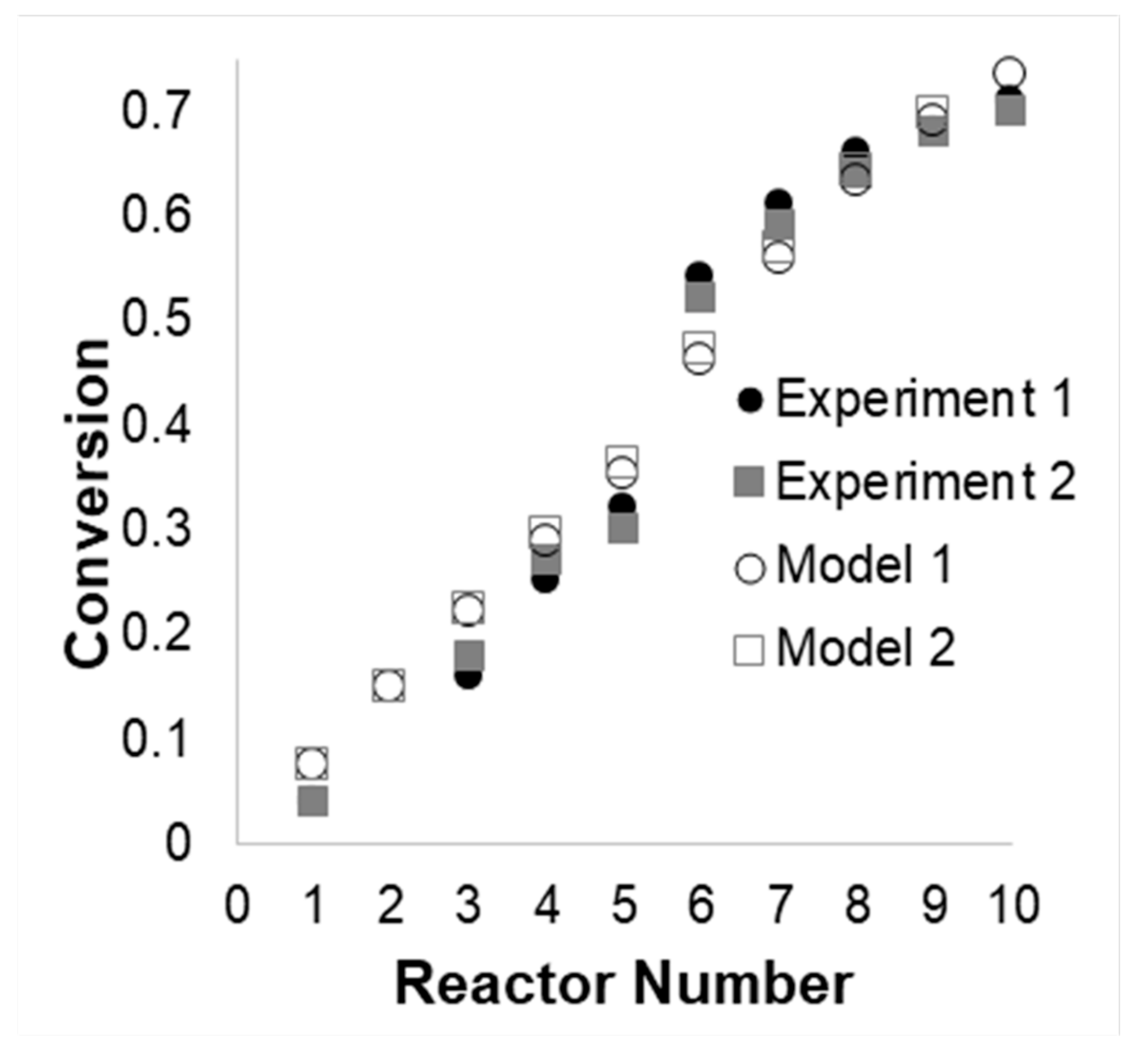
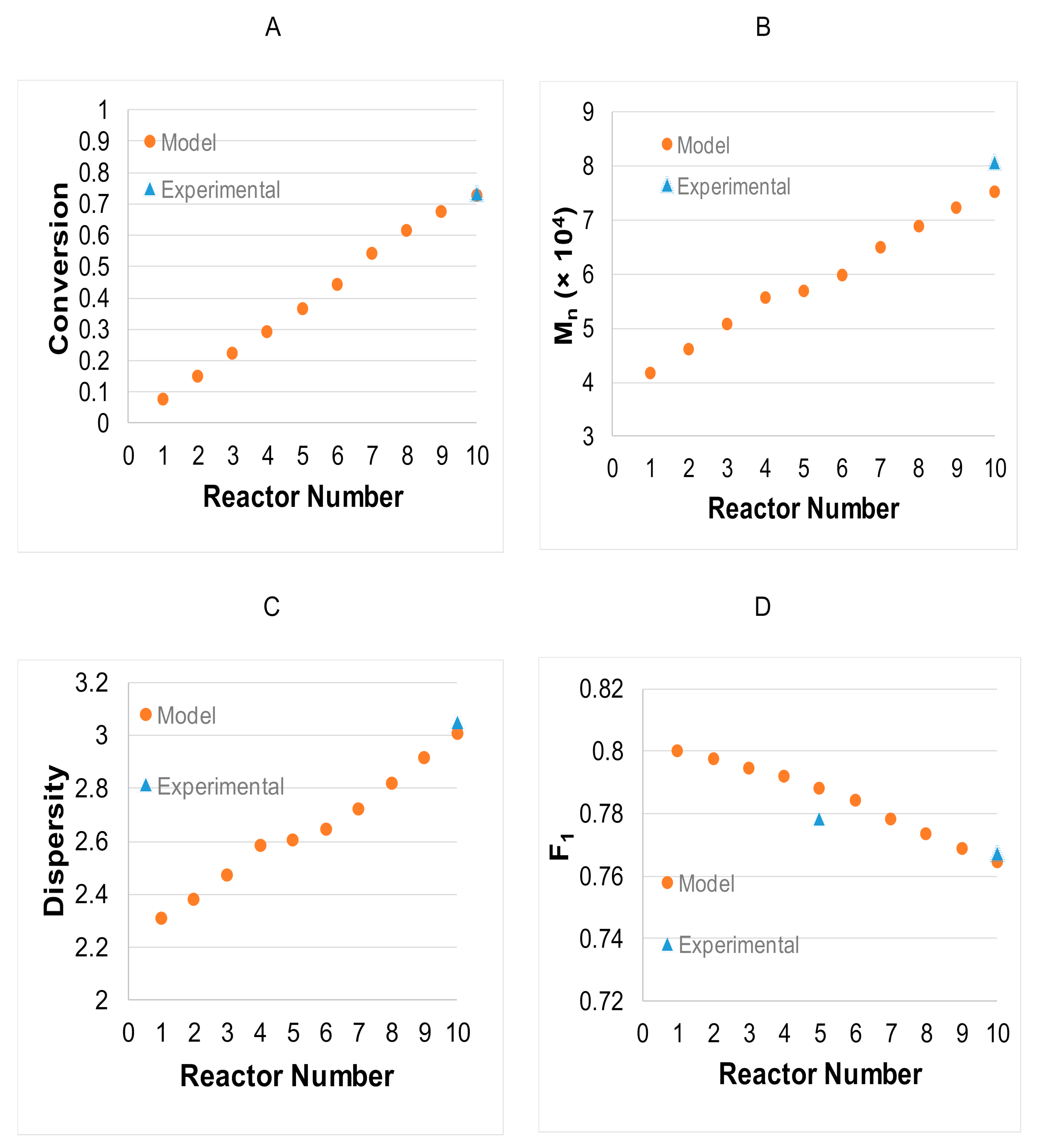
3.2. Model Validation

Figure 2 shows a comparison of the model predictions with plant data for conversion (18 experimental points) in the SBR case for a 10-reactor train. The steady-state operation of each reactor (except for reactor 2 (R2) in the train) was sampled at two different times (data labeled as experiments 1 and 2); slight temperature variations ( ±   1   C ) were recorded for the temperatures of the reactors at these different times, except for reactor 10, in which the temperature difference was +3 C for experiment 2. Details of the used temperature profile, as well as the formulation data used in the plant, are provided in Table 4. A similar formulation has been published before for the NBR case [29,32]. The agreement between model and experiment was quite reasonable using a single value of k m m = k m p .
Figure 3 shows the model predictions with a few experimental data from the plant available for the number average molecular weight M n , the MWD dispersity, and the accumulated copolymer composition F1. The copolymer composition was measured by refractive index (ASTM D5775-95(2019)), while M n and the MWD dispersity were measured by size exclusion chromatography (estimating absolute values from those relative to a polystyrene standard). The reactivity ratios were slightly adjusted (~10%) with respect to those reported in the open literature to get a better agreement with the copolymer composition data (Table 3), but this was justified since the literature data were obtained at a different temperature. The agreement of the model with the experimental data was reasonable but unfortunately limited to the few available experimental data points.
Figure 4, Figure 5 and Figure 6 show the effect of variation of surfactant on the most important outputs and process parameters with respect to the base case, which corresponded to the conditions of Experiment 1 and included a side stream of CTAs in R5. The predicted effects were all expected and easy to explain. As the surfactant increased with respect to the base value, more particles were produced (Figure 5A) and the reaction rate was higher (Figure 5C), as was the conversion (Figure 4A). At a higher conversion, the composition drift increased, as shown in Figure 4B–D. A higher number of particles resulted in smaller particle diameters (Figure 5D), although the effect is barely perceptible in the plot. Finally, higher reaction rates resulted in higher molecular weights and dispersities. The jump observed in Rp in R6 was due to the abrupt increase in temperature from R5 to R6 (+10 C). Figure 5B shows the value of the average number of radicals per particle ( n ˜ ) according to the model. It must be highlighted that some of the previous models ([3] and partially in [4,5]) assumed a constant value of n ˜ = 0.5 (Smith–Ewart case II kinetics), but, as seen in the figure, this may have deviated from the presumably true value by 20–30%, thus having a direct impact on the estimation of the polymerization rate (see Equation (5)).
Figure 6 shows how an increase in surfactant concentration also caused an increase in the average molecular weight (Figure 6A,B). This was due to an increased number of particles that delayed the entry of a second radical to the particle (more competition for radicals), extending its life and, therefore, its molecular weight. The increased competition for radicals also resulted in an increased dispersion in the probability of capturing a second radical, leading to increased MWD dispersity (Figure 6C). Notice that this explanation has also been put forward by other researchers, albeit in the frame of miniemulsion polymerization. [52,53]
Figure 7 shows the evolution of the number of particles with zero, one, and two radicals for the simulated SBR base case. At the first reactor, due to the relative abundance of initiator radicals, the number of particles with one radical (F1) was higher than that with zero radicals (F0); however, down the train, this situation was reversed as the initiator was depleted. From the plots, it is also clear that the number of particles with two radicals (F2) was negligible in all the reactors, pointing to the conclusion that a 0-1 model should suffice to represent these systems. Notice that this behavior does not mean that an average value of n ˜ = 0.5 would provide a good representation of the system as assumed in early models; it rather means that n ˜ < 0.5. However, the whole situation could change if a gel effect was included in the model.
Figure 8 shows the effect of the variation of the amount of CTAs on conversion, average molecular weights, and MWD dispersity. The effect was almost negligible on the conversion since the desorption of CTAs was not significant; however, the effect on the molecular weight averages and dispersity was as expected, with large increases in these quantities as the amount of CTAs decreased. The plot for a 45% decrease of CTAs is not shown since the calculation diverged for the last reactor as the system reached the gelation point (the second moment of the MWD tended to infinity).
Finally, Figure 9 shows the effect of the side stream of CTAs on the MWD. As mentioned above, in the base case, a (correction) side stream of CTAs was fed to R5. Figure 9 compares the behavior of the train with and without the intermediate CTA feed. As previously discussed, the effect was negligible for the progress of the conversion along the train (Figure 9A), but the final Mn and the dispersity increased from ~70,000 to ~90,000 and from ~7 to ~9, respectively, when the CTA side stream was suppressed. Similarly, the final number of branches increased from ~1 to ~1.2 in the absence of the side stream. Clearly, the intermediate CTA stream avoided an excessive increase in the molecular weight and the eventual formation of gel in the last reactors of the train that operate at high conversions.
The effects of the changes in the redox initiator system were milder than those found for the surfactant and CTAs and are shown in the Supplementary Materials (Figure S1).
Similar behavior was found for the NBR system upon changes in the surfactant, CTA, and initiator. The effects of changes in the surfactant for an NBR system are shown in Figure 10, Figure 11 and Figure 12 for the same important outputs and process parameters shown for the SBR system in Figure 4, Figure 5 and Figure 6. The variations of the surfactant were made with respect to a base case, which corresponded to a composition feed of f1 = 0.68 (wt. basis) and weight feed ratios of 1.25/0.082/0.35/100 for S/Iw/CTAs/monomers. The base case also included a side stream of an additional 20% flow rate of CTAs at R6. The used temperature was 10 °C in all reactors except in R1 (12 °C) and R10 (15 °C). The effects were very similar to those found for the SBR system, with a few exceptions. In Figure 10, the butadiene composition of the remaining monomer f1, as well as those of the copolymer (accumulated and instantaneous (F1 and F1,inst, respectively)), increased instead of decreasing like in the SBR case. This was expected given the differences in the reactivity ratios between the two systems. In this region of the monomer feed composition (above the azeotropic point for NBR) in the NBR case, acrylonitrile was consumed faster than butadiene (see the Mayo–Lewis plot for this system in Figure S2), and the composition of the remaining monomer therefore increased in butadiene with conversion, also leading to a richer butadiene composition in the copolymer.
The effects of the surfactant changes on N p , R p , n ˜ ,   and D p shown in Figure 11 for the NBR system were qualitatively very similar to those observed and already discussed for the SBR case (Figure 5). The only minor difference was that the effects were smaller for n ˜   in the NBR than in the SBR case. Another difference is that in the NBR case, there was not a jump in the reaction rate as in the SBR case; however, this was simply because in the former case, there was not a jump in an intermediate reactor temperature as in the latter. Figure 12 shows similar effects of the surfactant concentration for the NBR system compared to those in the SBR system (Figure 6). A difference was that in the NBR case, the molecular weights reached a peak in R5 to decrease in R6 due to the side stream of CTAs. This effect was less important in the SBR base case, but in that system, the higher temperatures in the last reactors also significantly contributed to higher molecular weights. Additionally, the molecular weights and dispersities were lower for NBR compared to those exhibited by the SBR system.
The effects of changes in the CTA feed with respect to the NBR base case are shown in Figure 13, which is comparable to Figure 8 for the SBR system. Again, the behavior of both systems was qualitatively similar with the only exception of the peak exhibited by the molecular weights in R5 for the NBR case due to the side stream of CTAs in R6, as in Figure 12, and the different temperature profiles used for the SBR and the NBR cases.
More interesting behavior for the NBR system was related to the drift in copolymer composition along the train. Given the reactivity ratios of this system (0.30 and 0.04), the system exhibited an azeotropic composition at f1,az = F1,az = 0.578 (molar basis, 0.582 weight basis) (see the F1 vs. f1 Mayo–Lewis curve in the Supplementary Materials, Figure S2) Therefore, composition drift depends on what side of the azeotrope the composition of the feed is located. If the feed composition is above f1,az, as in most commercial grades of NBR, without correction, the instantaneous product composition will initially deviate towards copolymers with a lower Bd composition than the feed (R1); however, as the reaction mixture proceeds along the reactor train, the Bd-enriched environment will tend to increase the Bd content in the copolymer. This can be seen in Figure 14 for a product grade in which f1 in the feed was 0.68 (wt. basis). Since composition drift may lead to a product with heterogeneous composition or a product deviated from the target average composition, it is common to introduce a side feed stream of AN in an intermediate reactor of the train to “correct” or attenuate the composition drift. Figure 10 also shows the composition profile when an additional AN side stream (20% of the initial feed) was fed to reactor R7. Without the correction, the final F1 was above 0.66; on the other hand, with the side feed stream at R7, the final F1 was slightly below 0.65. A second example is shown in Figure 15; in this case, the composition of the feed was f1 = 0.5 on a wt. basis, a composition which was located on the other side of the azeotrope (see the F1 vs. f1 curve in the Supplementary Materials). The behavior of this system was the opposite of that in the previous example, exhibiting a composition drift that initially produced copolymers with a higher Bd composition than the feed (R1, F1 ~0.58) and a decreasing Bd content in the copolymer along the reactor train to end up with an F1 slightly above 0.56, although the instantaneous F1 fell below 0.54 at R10. Figure 15 also shows how this drift could be attenuated by feeding a side stream of Bd (20% of the initial feed). This correction worked very well, resulting in a final average composition near the target (F1 ~0.58) while avoiding large deviations in the instantaneous composition produced in each reactor (better composition homogeneity).

4. Conclusions

A single mechanistic model was built and used to describe the production of both SBR and NBR elastomers in trains of emulsion polymerization CSTRs. The aim was to balance the level of complexity of the model with its capability of describing the effects observed at the plant on the process parameters in a quantitative way and the product quality upon variable changes. Some novel aspects of this model compared to previous models are summarized below, along with additional comments:
-
The radical compartmentalization was considered in more detail, both in the particle kinetics description and in the calculation of the moments of the MWD, and for the first time, a 0-1-2 model was used to describe these two important aspects in these processes. It was found that at least a 0-1 model should be used for an accurate description of the compartmentalization effects, especially for the first reactors in the train. A similar conclusion was recently put forward by Marien et al. [52] using stochastic simulation, although for a general miniemulsion system.
-
The monomer partitioning model was as simple as possible, and its parameters could be estimated a priori based on published physicochemical data. As mentioned by Madhuranthakam and Penlidis, [30] the use of more sophisticated thermodynamic models for monomer partitioning seems to be unnecessary for this kind of system.
-
A single modeling framework was presented in a unified form for the SBR and NBR systems. Though previous models have been applied with adaptations to both systems in some series of papers, it is believed that by presenting them together, it is easier to appreciate the similarities and differences in both systems.
The model is presently used in the plant to design changes of configurations of the reactor train, such as the number of reactors in the train (up to 16 reactors in the existing facility), the reactor volume, the location and flows of side streams of CTAs and monomers, and grade recipes, among other variables, to maximize the plant operation versatility maintaining high productivity and product quality. The model is quite flexible, and it has been implemented with the help of a friendly graphical interphase. Current work involves the generation of product quality correlations that link model outputs, e.g., Mn and Mw, and number of branches, with product performance parameters, such as Mooney viscosity.

Supplementary Materials

The following are available online at https://www.mdpi.com/2227-9717/8/11/1508/s1, File with figures and additional equations.

Author Contributions

Conceptualization, E.S.-G. and J.M.I.-M.; methodology, E.S.-G., R.I.-M., and J.M.I.-M; software, E.S.-G. and R.I.-M.; validation, E.S.-G., R.I.-M., and J.M.I.-M.; writing—original draft preparation, E.S.-G. and J.M.I.-M; writing—review and editing, E.S.-G. and J.M.I.-M.; project administration, E.S.-G. and J.M.I.-M; funding acquisition, E.S.-G. and J.M.I.-M. All authors have read and agreed to the published version of the manuscript.

Funding

This research was funded by Dynasol Elastomers and the publication fee by CIQA.

Acknowledgments

The authors thank Dynasol Elastomers for industrial data and CIQA for administrative support.

Conflicts of Interest

The authors declare no conflict of interest.

References

  1. Production Capacity of Styrene-Butadiene-Rubber Worldwide in 2018 and 2023. Available online: https://www.statista.com/statistics/1063647/styrene-butadiene-rubber-production-capacity-globally/ (accessed on 8 January 2020).
  2. The Global Nitrile Butadiene Rubber (NBR) Market to 2023: Global Production of NBR is Likely to Reach ~1,562 Thousand Tons. Available online: https://www.businesswire.com/news/home/20181126005386/en/Global-Nitrile-Butadiene-Rubber-NBR-Market-2023 (accessed on 8 January 2020).
  3. Kanetakis, J.; Wong, F.Y.C.; Hamielec, A.E.; MacGregor, J.F. Steady State Modeling of a Latex Reactor Train for the Production of Styrene-Butadiene Rubber. Chem. Eng. Commun. 1985, 35, 123–140. [Google Scholar] [CrossRef]
  4. Broadhead, T.O.; Hamielec, A.E. Dynamic modelling of the batch, semi-batch and continuous production of styrene/butadiene copolymers by emulsion polymerization. Die Makromol. Chem. 1985, 10, 105–128. [Google Scholar] [CrossRef]
  5. Penlidis, A.; MacGregor, J.F.; Hamielec, A.E. Dynamic modelling of emulsion polymerization reactors. AIChE J. 1985, 31, 881–889. [Google Scholar] [CrossRef]
  6. Smith, W.V.; Ewart, R.H. Kinetics of Emulsion Polymerization. J. Chem. Phys. 1948, 16, 592–599. [Google Scholar] [CrossRef]
  7. Storti, G.; Carrá, S.; Morbidelli, M.; Vita, G. Kinetics of multimonomer emulsion polymerization. The pseudo-homopolymerization approach. J. Appl. Polym. Sci. 1989, 37, 2443–2467. [Google Scholar] [CrossRef]
  8. Tobita, H.; Hamielec, A.E. Kinetics of free-radical copolymerization: The pseudo-kinetic rate constant method. Polymer 1991, 32, 2641–2647. [Google Scholar] [CrossRef]
  9. Saldívar, E.; Dafniotis, P.; Ray, W.H. Mathematical Modeling of Emulsion Copolymerization Reactors. I. Model Formulation and Application to Reactors Operating with Micellar Nucleation. J. Macromol. Sci. Part C Polym. Rev. 1998, 38, 207–325. [Google Scholar] [CrossRef]
  10. Ugelstad, J.; Mork, P.C.; Aasen, J.E. Kinetics of emulsion polymerization. J. Polym. Sci. 1967, A5, 2281–2288. [Google Scholar] [CrossRef]
  11. Yabuki, Y.; MacGregor, J.F. Product Quality Control in Semibatch Reactors Using Midcourse Correction Policies. Ind. Eng. Chem. Res. 1997, 36, 1268–1275. [Google Scholar] [CrossRef]
  12. Gugliotta, L.M.; Brandolini, M.C.; Vega, J.R.; Iturralde, E.O.; Azum, J.L.; Meira, G.R. Dynamic Model of a Continuous Emulsion Copolymerization of Styrene and Butadiene. Polym. React. Eng. 1995, 3, 201–233. [Google Scholar]
  13. Flory, P.J. Principles of Polymer Chemistry; Cornell University Press: Ithaca, NY, USA, 1953. [Google Scholar]
  14. Morton, M.; Kaizerman, S.; Altier, M.W. Swelling of latex particles. J. Colloid Sci. 1954, 9, 300–312. [Google Scholar] [CrossRef]
  15. Vega, J.R.; Gugliotta, L.M.; Brandolini, M.C.; Meira, G.R. Steady-State Optimization in a Continuous Emulsion Copolymerization of Styrene and Butadiene. Lat. Am. Appl. Res. 1995, 25, 207–214. [Google Scholar]
  16. Vega, J.R.; Gugliotta, L.M.; Meira, G.R. Continuous Emulsion Polymerization of Styrene and Butadiene. Reduction of Off-Spec Product between Steady-State. Lat. Am. Appl. Res. 1995, 25, 77–82. [Google Scholar]
  17. Minari, R.J.; Vega, J.R.; Gugliotta, L.M.; Meira, G.R. Continuous Emulsion Styrene-Butadiene Rubber (SBR) Process: Computer Simulation Study for Increasing Production and for Reducing Transients between Steady States. Ind. Eng. Chem. Res. 2006, 45, 245–257. [Google Scholar] [CrossRef]
  18. Godoy, J.L.; Minari, R.J.; Vega, J.R.; Marchetii, J.L. Multivariate statistical monitoring of an industrial SBR process. Soft-sensor for production and rubber quality. Chemom. Intell. Lab. Syst. 2011, 107, 258–268. [Google Scholar] [CrossRef]
  19. Zubov, A.; Pokorny, J.; Kosek, J. Styrene–butadiene rubber (SBR) production by emulsion polymerization: Dynamic modeling and intensification of the process. Chem. Eng. J. 2012, 207, 414–420. [Google Scholar] [CrossRef]
  20. Mustafina, S.; Miftakhov, E.; Mikhailova, T. Mathematical Study of Copolymer Composition and Compositional Heterogeneity during the Synthesis of Emulsion-Type Butadiene-Styrene Rubber. Int. J. Chem. Sci. 2014, 12, 1135–1144. [Google Scholar]
  21. Dubé, M.A.; Penlidis, A.; Mutha, R.K.; Cluett, W.R. Mathematical Modeling of Emulsion Copolymerization of Acrylonitrile/Butadiene. Ind. Eng. Chem. Res. 1996, 46, 4434–4448. [Google Scholar] [CrossRef]
  22. Vega, J.R.; Gugliotta, L.M.; Bielsa, R.O.; Brandolini, M.C.; Meira, G.R. Emulsion Copolymerization of Acrylonitrile and Butadiene. Mathematical Model of an Industrial Reactor. Ind. Eng. Chem. Res. 1997, 36, 1238–1246. [Google Scholar] [CrossRef]
  23. Rodríguez, V.I.; Estenoz, D.A.; Gugliotta, L.M.; Meira, G.R. Emulsion Copolymerization of Acrylonitrile and Butadiene. Calculation of the Detailed Macromolecular Structure. Int. J. Polym. Mater. 2002, 51, 511–529. [Google Scholar] [CrossRef]
  24. Vega, J.R.; Gugliotta, L.M.; Meira, G.R. Emulsion Copolymerization of Acrylonitrile and Butadiene. Semibatch Strategies for Controlling Molecular Structure on the Basis of Calorimetric Measurements. Polym. React. Eng. 2002, 10, 59–82. [Google Scholar] [CrossRef]
  25. Minari, R.J.; Gugliotta, L.M.; Vega, J.R.; Meira, G.R. Continuous emulsion copolymerization of acrylonitrile and butadiene: Computer simulation study for improving the rubber quality and increasing production. Comput. Chem. Eng. 2007, 31, 1073–1080. [Google Scholar] [CrossRef]
  26. Minari, R.J.; Gugliotta, L.M.; Vega, J.R.; Meira, G.R. Continuous emulsion copolymerization of acrylonitrile and butadiene: Simulation study for reducing transients during changes of grade. Ind. Eng. Chem. Res. 2007, 46, 7677–7683. [Google Scholar] [CrossRef]
  27. Clementi, L.A.; Suvire, R.B.; Rossomando, F.G.; Vega, J.R. A Closed-Loop Control Strategy for Producing Nitrile Rubber of Uniform Chemical Composition in a Semibatch Reactor: A Simulation Study. Macromol. React. Eng. 2018, 12, 1700054. [Google Scholar] [CrossRef]
  28. Washington, I.D. Dynamic Modelling of Emulsion Polymerization for the Continuous Production of Nitrile Rubber. Master’s Thesis, University of Waterloo, Waterloo, ON, Canada, 2008. [Google Scholar]
  29. Washington, I.D.; Duever, T.A.; Penlidis, A. Mathematical Modeling of Acrylonitrile-Butadiene Emulsion Copolymerization: Model Development and Validation. J. Macromol. Sci. Part A Pure Appl. Chem. 2010, 47, 747–769. [Google Scholar] [CrossRef]
  30. Madhuranthakam, C.M.R.; Penlidis, A. Modeling Uses and Analysis of Production for Acrylonitrile-Butadiene (NBR) Emulsions. Polym. Eng. Sci. 2011, 51, 1909–1918. [Google Scholar] [CrossRef]
  31. Madhuranthakam, C.M.R.; Penlidis, A. Improved Operating Scenarios for the Production of Acrylonitrile-Butadiene Emulsions. Polym. Eng. Sci. 2012, 53, 9–20. [Google Scholar] [CrossRef]
  32. Scott, A.J.; Nabifar, A.; Madhuranthakam, C.M.R.; Penlidis, A. Bayesian Design of Experiments Applied to a Complex Polymerization System: Nitrile Butadiene Rubber Production in a Train of CSTRs. Macromol. Theory Simul. 2015, 24, 13–27. [Google Scholar] [CrossRef]
  33. Vale, H.M.; McKenna, T.F. Synthesis of bimodal PVC latexes by emulsion polymerization: An experimental and modeling study. Macromol. Symp. 2006, 243, 261–267. [Google Scholar] [CrossRef]
  34. Dubé, M.A.; Saldívar-Guerra, E.; Zapata-González, I. Copolymerization. In Handbook of Polymer Synthesis, Characterization and Processing; Saldívar-Guerra, E., Vivaldo-Lima, E., Eds.; John Wiley and Sons: Hoboken, NJ, USA, 2013. [Google Scholar]
  35. Blackley, D.C. Emulsion Polymerization; Applied Science Publishers: London, UK, 1975. [Google Scholar]
  36. Friis, N.; Nyhagen, L. A Kinetic Study of the Emulsion Polymerization of Vinyl Acetate. J. Appl. Polym. Sci. 1973, 17, 2311–2327. [Google Scholar] [CrossRef] [Green Version]
  37. Nomura, M. Desorption and Reabsorption of Free Radicals in Emulsion Polymerization. In Emulsion Polymerization; Piirma, I., Ed.; Academic Press: New York, NY, USA, 1982; pp. 191–219. [Google Scholar]
  38. Dougherty, E. The SCOPE Dynamic Model for Emulsion Polymerization. I. Theory. J. Appl. Polym. Sci. 1986, 32, 3051–3078. [Google Scholar] [CrossRef]
  39. Gardon, J.L. Emulsion polymerization. VI. Concentration of monomers in latex particles. J. Polym. Sci. Part A-1 Polym. Chem. 1968, 6, 2859–2879. [Google Scholar] [CrossRef]
  40. Ascher, U.M.; Petzold, L.R. Computer Methods for Ordinary Differential Equations and Differential-Algebraic Equations; Society for Industrial and Applied Mathematics: Philadelphia, PA, USA, 1998. [Google Scholar]
  41. Buback, M.; Gilbert, R.G.; Hutchinson, R.A.; Klumperman, B.; Kuchta, F.-D.; Manders, B.G.; O’Driscoll, K.F.; Russell, G.T.; Schweer, J. Critically evaluated rate coefficients for free-radical polymerization, 1. Propagation rate coefficients for styrene. Macromol. Chem. Phys. 1995, 196, 3267–3280. [Google Scholar] [CrossRef] [Green Version]
  42. Junkers, T.; Koo, S.P.S.; Barner-Kowollik, C. Determination of the propagation rate coefficient of acrylonitrile. Polym. Chem. 2010, 1, 438–441. [Google Scholar] [CrossRef]
  43. Saldívar, E.; Araujo, O.; Giudici, R.; López-Barrón, C. Modeling and Experimental Studies of Emulsion Copolymerization Systems. II. Styrenics, J. Appl. Polym. Sci. 2001, 79, 2380–2397. 2001, 79, 2380–2397. [Google Scholar]
  44. Deibert, S.; Bandermann, F.; Schweer, J.; Sarnecki, J. Propagation rate coefficient of free-radical polymerization of 1,3-butadiene. Makromol. Chem. Rapid Commun. 1992, 13, 351–355. [Google Scholar] [CrossRef]
  45. Bachmann, R.; Pallaske, U.; Schmidt, A.; Muller, H.G. DECHEMA Monographs; VCH: Weinham, Germany, 1995; Volume 131, pp. 65–74. [Google Scholar]
  46. Deibert, S.; Bandermann, F. Rate coefficients of the free-radical polymerization of 1,3-butadiene. Die Makromol. Chem. 1993, 194, 3287–3299. [Google Scholar] [CrossRef]
  47. Brandrup, J.; Immergut, E.H.; Grulke, E.A. (Eds.) Polymer Handbook, 4th ed.; John Wiley and Sons: New York, NY, USA, 1994. [Google Scholar]
  48. Mukerjee, P.; Mysels, K.J. Critical Micelle Concentrations of Aqueous Surfactant Systems; NSRDS-NBS 36; National Bureau of Standards: Washington, DC, USA, 1971. [Google Scholar]
  49. Rawlings, J.B.; Ray, W.H. The modeling of batch and continuous emulsion polymerization reactors. Part II: Comparison with experimental data from continuous stirred tank reactors. Polym. Eng. Sci. 1988, 28, 257–274. [Google Scholar] [CrossRef]
  50. Arve, D.S.C.; Manley, D.B.; Poling, B.E. Relative volatilities from mixture liquid densities for the n-butane/1,3-butadiene system. Fluid Phase Equilib. 1987, 35, 117–126. [Google Scholar] [CrossRef]
  51. Guyot, A.; Guillot, J.; Graillat, C.; Llauro, M.F. Controlled composition in emulsion copolymerization application to butadiene-acrylonitrile copolymers. J. Macromol. Sci.-Chem. 1984, A21, 683–699. [Google Scholar] [CrossRef]
  52. Marien, Y.W.; Van Steenberge, P.H.M.; D’hooge, D.; Marin, G.B. Particle by Particle Kinetic Monte Carlo Tracking of Reaction and Mass Transfer Events in Miniemulsion Free Radical Polymerization. Macromolecules 2019, 52, 1408–1423. [Google Scholar] [CrossRef]
  53. Marien, Y.W.; Van Steenberge, P.H.M.; Pich, A.; D’hooge, D. Coupled stochastic simulation of the chain length and particle size distribution in miniemulsion radical copolymerization of styrene and N-vinylcaprolactam. React. Chem. Eng. 2019, 4, 1935–1947. [Google Scholar] [CrossRef]
Figure 1. Data flow and computer programs for the implementation of the numerical solution of the mathematical model. Each stage (darker blocks) represents a computer program that is run separately and sequentially. See the text for more details.
Processes 08 01508 g001
Figure 2. Comparison of plant conversion data with model predictions for two operating conditions. The two simulated operating conditions are indicated as Model 1 and Model 2, See the conditions in Table 4.
Processes 08 01508 g002
Figure 3. Comparison of model prediction with plant experimental data for conversion (A), number average molecular weight instantaneous (Mn) (B), MWD dispersity (C), and accumulated copolymer composition F1 (D). The parameter values were those in Table 3, and the reaction conditions were similar to those in Table 4.
Processes 08 01508 g003
Figure 4. Effect of variation of surfactant (from −45% to +45%) on conversion (A), remaining monomer feed composition f1 (B), instantaneous copolymer composition (F1,inst) (C), and accumulated copolymer composition F1 (D) along the reactor train with respect to the base case in SBR production. All compositions are weight fractions.
Processes 08 01508 g004
Figure 5. Effect of variation of surfactant (from −45% to +45%) on number of particles Np (A), average number of radicals n ˜ (B), reaction rate Rp (C), and particle diameter Dp (D) along the reactor train with respect to the base case in SBR production.
Processes 08 01508 g005
Figure 6. Effect of variation of surfactant (from −45% to +45%) on the number-average molecular weight Mn (A), weight-average molecular weight Mw (B), and MWD dispersity (C) along the reactor train with respect to the base case in SBR production.
Processes 08 01508 g006
Figure 7. Number of particles with zero (F_0), one (F_1), and two (F_2) radicals per L of water at each reactor for the SBR base case. (A) Linear scale; (B) log scale.
Processes 08 01508 g007
Figure 8. Effect of variation of chain transfer agents (CTAs) (from −30% to +45%) on the conversion (A), number-average molecular weight Mn (B), weight-average molecular weight Mw (C), and MWD dispersity (D) along the reactor train with respect to the base case in SBR production.
Processes 08 01508 g008
Figure 9. Effect of suppressing the side stream of CTAs of the base case on the conversion (A), number-average molecular weight Mn (B), MWD dispersity (C), and number of branches per chain (D) along the reactor train with respect to the base case (corrected) in SBR production.
Processes 08 01508 g009
Figure 10. Effect of variation of surfactant (from −45% to +45%) on conversion (A), remaining monomer feed composition f1 (B), instantaneous copolymer composition (F1,inst) (C), and accumulated copolymer composition F1 (D) along the reactor train with respect to the base case in NBR production. All compositions are weight fractions.
Processes 08 01508 g010
Figure 11. Effect of variation of surfactant (from −45% to +45%) on number of particles Np (A), average number of radicals n ˜ (B), reaction rate Rp (C), and particle diameter Dp (D) along the reactor train with respect to the base case in NBR production.
Processes 08 01508 g011
Figure 12. Effect of variation of surfactant (from −45% to +45%) on the number-average molecular weight Mn (A), weight-average molecular weight Mw (B), and MWD dispersity (C) along the reactor train with respect to the base case in NBR production.
Processes 08 01508 g012
Figure 13. Effect of variation of CTAs (from −45% to +45%) on the conversion (A), number-average molecular weight Mn (B), weight-average molecular weight Mw (C), and MWD dispersity (D) along the reactor train with respect to the base case in NBR production.
Processes 08 01508 g013
Figure 14. Effect of the operation of the reactor train for NBR production with (corrected) and without a side stream of additional AN in R7 (20% with respect to the AN feed in R1) on conversion (A) and instantaneous butadiene copolymer composition (F1,inst) and accumulated butadiene copolymer composition (F1) (B). The initial monomer feed was f1 = 0.68 (wt. basis).
Processes 08 01508 g014
Figure 15. Effect of the operation of the reactor train for NBR production with (corrected) and without a side stream of additional Bd in R7 (20% with respect to the Bd feed in R1) on conversion (A) and instantaneous butadiene copolymer composition (F1,inst) and accumulated butadiene copolymer composition (F1) (B). The initial monomer feed is f1 = 0.5 (wt. basis).
Processes 08 01508 g015
Table 1. Kinetics in the aqueous and particle phase.
ReactionKinetics
Aqueous phase
Redox initiation I w + Y 1 r k d 1   R w + Y 1 o + p r o d u c t s
Y 1 o +   Y 2 k d 2   Y 1 r + p r o d u c t s
R w +   M w   k p ¯   P w
P w + M w   k p ¯ P w
P w P w k t ¯ D w
Particle phase, detailed terminal model 1
Propagation and cross-propagation (i,j = 1,2) P i + M j k p , i j P j
Chain transfer to monomer (i,j = 1,2) P i + M j k t r M i j   P j + D
Chain transfer to chain transfer agent T (i,j = 1,2) P i + T k t r T i   P i + D
Particle phase, molecular weight distribution (MWD) pseudo-homopolymer form 2
Propagation (r = 1, …, ∞) P r + M k p ¯ P r + 1
Chain transfer to monomer (r = 1, …, ∞) P r + M k t r M   ¯ P 1 + D r
Chain transfer to chain transfer agent (r = 1, …, ∞) P r + T k t r T   ¯ P 1 + D r
Termination by combination and disproportionation (r,q = 1, …, ∞) 2 P r + P q k t c ¯ D r + q
P r + P q k t d ¯ D r + D q
Chain transfer to polymer (q,r = 1,..,∞) 3 P q + D r     r k t r p ¯ P r + D q
Internal or terminal double bond polymerization (q,r = 1, …, ∞) 3 P q + D r     F 1 , m o c r k d b P r + q
1 A pseudo-homopolymer approach with apparent rate constants is used to represent the copolymerization kinetics based on the terminal model. 2 A single value k t ¯ = k t c ¯ + k t d ¯ was used for the termination step, calculated as k t ¯ = k t 11 k t 22 while assuming diffusion-controlled termination, where k t j j ,   j = 1 , 2 ,   are the homotermination constants for monomers 1 and 2. 3 The transfer-to-polymer and double bond polymerization reactions are only considered for the MWD calculations.
Table 2. Working equations for implementation in the solution code.
VariableEquation(s)Number of Equations
Ordinary differential equations (ODEs) (mass or population balance equations)
Monomers, M i 12
Monomer bound in polymer, H i 22
Initiator, I w 121
Reducing agent 1, Y 1 131
Reducing agent 2, Y 2 141
Surfactant, S 151
Chain transfer agent, T r 181
Water, W 201
Number of particles con n radicals, F n 7–93
Live polymer momentsSupplementary Material Equations (S3f)–(S3i) with extensions Supplementary Material Equation (S3u), Supplementary Material Equation (S3v), Supplementary Material Equation (S3x), and Supplementary Material Equation (S3y)4
Dead polymer momentsSupplementary Material Equations (S3j)–(S3r) with extensions Supplementary Material Equations (S3aa)–(S3af)9
TOTAL ODEs26
Main auxiliary (algebraic) equations
Radicals in the aqueous phase, P w 211
Number of micelles per L of water, M i c 16 or 171
Entry coefficient of radicals to particles, ρ Supplementary Material Equation (S1a)1
Entry coefficient of radicals to micelles, ρ m i c Supplementary Material Equation (S1b)1
Desorption coefficient, k d e s Supplementary Material Equation (S1c)1
Chain transfer agent (CTA) concentration in particles, T r p Supplementary Material Equation (S1aa)1
Monomer concentration in particles, M p 23 or 251
Total mass, M T 291
Number of branches per chain, B 361
Closure expression for 3rd momentsSupplementary Material Equation (S3ag)1
Total number of algebraic equations10
Table 3. Parameter values tested or used in the simulations for the styrene–butadiene rubber (SBR) and acrylonitrile–butadiene rubber (NBR) systems.
ParameterValueUnitsSource/Comments
SBR System: monomer 1 butadiene, monomer 2 styrene
r11.4–1.58 1.4 from [46] (@ 50 C)
r20.54–0.58 0.58 from [46] (@ 50 C)
1E, k p , 11 8540cal mol−1[47]
1A, k p , 11 1.12 × 10⁸L mol−1 s−1[47]
2E, k p , 22 6220cal mol−1[46]
2A, k p , 22 4.50 × 10⁶L mol−1 s−1[46]
E, k p , 22 7770cal mol−1[41] Pulse laser polymerization (PLP)-determined
A, k p , 22 4.27 × 10⁷L mol−1 s−1[41] PLP-determined
k d 1 100–250L mol−1 s−1Estimated
k d 2 50–200L mol−1 s−1Estimated
k t , 11 @ 10 C9.16 × 108L mol−1 s−1[45] PLP-determined
k t , 22 @ 10 C9.2 × 106L mol−1 s−1[46]
C M 1 9 × 10⁻⁵-Estimated from [46]
C M 2 9 × 10⁻⁵-Assumed equal to C M 1
C T 1 2-Estimated
C T 2 2-Estimated
r m 5 × 10⁻⁹mEstimated
S c m c 9.8 × 10⁻⁴mol L−1[48]
a e m 2.2 × 10⁻¹⁹m2Estimated
b2000L mol−1[9]
  Γ 3.5 × 10⁻⁶mol m−2[9]
x s a t 0.55-Estimated
f0.5-Estimated
k m m This work
k m p This work
D w 3.55 × 10⁻¹⁵m2 s−1[49]
D p 3.55 × 10⁻¹⁵m2 s−1[49]
D w T 2 × 10⁻¹⁵m2 s−1Estimated
D p T 2 × 10⁻¹⁵m2 s−1Estimated
m d 20 Estimated
m d T 100 Estimated
K T 200 Estimated
k t r p 0.005–0.05L mol−1 s−1This work
ρ 1 618g L−1Estimated from [50]
ρ 2 906g L−1[49]
ρ p 1 910g L−1Estimated from MSDS Sigma Aldrich St. Louis MOpolybutadiene Mw = 200,000
ρ p 2 1040g L−1[46]
Density surfactant918g L−1Estimated
NBR System: monomer 1 butadiene, monomer 2 acrylonitrile
3NBR System: monomer 1 butadiene, monomer 2 acrylonitrile 3
r10.30 [51]
r20.04 [51]
2 k p , 22 6633L mol−1 s−1[24]
E, k p , 22 3690cal mol−1[42] PLP-determined
A, k p , 22 1.83 × 10⁶L mol−1 s−1[42] PLP-determined
k t , 22 @ 10 C3.4 × 107L mol−1 s−1[28]
S c m c 6.5 × 10⁻⁴mol L−1[48]
a e m 3.8 × 10⁻¹⁹m2Estimated
m d 10 Estimated
ρ 2 822g L−1[28] @ 10 C
ρ p 2 1167g L−1[28] @ 10 C
χ A N 3.5 Estimated
1 In all kinetic constants kx where an Arrhenius expression was available, the used notation is: k x = A exp E R T with R = 1.987 cal mol−1 K−1 and the temperature T in K. 2 Values used in all the simulations in figures. 3 Only the used values that are different from those of the SBR system are listed.
Table 4. Typical recipe in parts per hundred monomer (pphm). Approximately the medium value of the range for each component was used in the simulations.
ComponentParts per Hundred Monomer (pphm)
Butadiene (M1)72
Styrene (M2)28
Initiator0.1–0.2
Reducing agent 1 10.02–0.05
Reducing agent 2 20.04–0.10
Chain transfer agent0.10–0.17
Surfactant3.0–5.0
Caustic potash0.5–0.7
Electrolyte (sodium carbonate, potassium chloride)0.2–0.4
Reactor NoR1–R5R6R7R8R9–R10
TemperaturebaseT (Tb)Tb + 10 CTb + 7 CTb + 6 CTb + 2 C
1 Based on ferrous sulfate. 2 Based on sodium formaldehyde sulfoxylate.
Publisher’s Note: MDPI stays neutral with regard to jurisdictional claims in published maps and institutional affiliations.

