A Reference-Model-Based Neural Network Control Method for Multi-Input Multi-Output Temperature Control System

Abstract

Neural networks (NNs), which have excellent ability of self-learning and parameter adjusting, has been widely applied to solve highly nonlinear control problems in industrial processes. This paper presents a reference-model-based neural network control method for multi-input multi-output (MIMO) temperature system. In order to improve the learning efficiency of the NN control, a reference model is introduced to provide the teaching signal for the NN controller. The control inputs for the MIMO system are given by the sum of the output of the conventional integral-proportional-derivative (I-PD) controller and the outputs of the neural network controller. The proposed NN control method can not only improve the transient response of the system, but can also realize temperature uniformity in MIMO temperature systems. To verify the proposed method, simulations are carried out in MATLAB/SIMULINK environment and experiments are carried out on the DSP (Digital Signal Processor)-based experimental platform, respectively. Both results are quantitatively compared to those obtained from the conventional I-PD control systems. The effectiveness of the proposed method has been successfully verified.

1. Introduction

To realize the precise temperature of the industrial process, temperature controllers are widely applied to manage manufacturing processes and operations. The common uses include food processing, packaging machines, and plastic extrusion etc. Their performances can seriously affect product quality, energy consumption, and production cost. In practical application, the proportional-integral-derivative (PID) controller has been widely used for its simple structure and wide applicability, especially in linear systems or first and second order systems [1]. Common methods for determining PID controller parameters are Ziegler–Nichols (ZN) and Cohen–Coon tuning rules, which are widely used in the industry due to their simplicity and ease of implementation, but may easily result in overshoot and weak response damping [2]. Meanwhile, most industrial processes are multi-variable nonlinear systems with big time constants, strong coupling effects, and large time delays. For such controlled objects, only using the conventional PID controller may not satisfy the requirements of the system performance.

In order to ensure the robustness and stability of the controller, many methods have been proposed to improve the performance of the PID controller, such as gain and phase margin [3], pole placement [4], and internal model control (IMC) [5]. For canceling the coupling interactions between each channels in multi-input multi-output (MIMO) systems, a verity of decoupling control strategies have been applied, such as inverse Nyquist array(INA) [6], feedforward decoupling control [7], and inverse based decoupling control [8]. These decoupling control methods are to design the decoupler so that the MIMO control system can be divided into multiple single-input single-output (SISO) loops, which allows one to adopt well developed single loop control methods. However, the modeling error may decrease system performance as decoupling is guaranteed under the condition that the precise mathematical model is obtained. The quality of the obtained model depends on many on-site factors, such as the excitation condition and selected identification algorithm [9,10,11]. In addition, the decoupling control is not enough to reach uniform temperature control in transient state without adjusting the PID parameters in different channels [12].

Considering the complex control rules and controller computation grow exponentially with a number of variables in nonlinear MIMO systems, intelligent control strategies are developed and widely used. Fuzzy logic control, genetic algorithms, and neural networks (NN) are the most promising methods among them [13,14,15]. NN is known for its great computing power and learning ability to emulate various systems dynamics with a highly parallel structure. Over the past few decades, NN has been successfully applied in many fields such as system modeling, pattern recognition, and signal processing [16,17,18,19]. In thermal systems, the NN has been used for heat transfer data analysis, performance prediction, and dynamic modeling etc. [20,21,22,23]. It is shown that NN is well suitable to deal with complex nonlinear relationships in control systems. NN helps solve the problem in typical heating system control methods that once the parameters of the control system are designed, they cannot be adjusted while the system is in operation. For a thermal process system with strong nonlinearly, large lag, and strong coupling, an adaptive system can improve control performance in terms of the transient response and overshoot [24,25,26].

Our previous research has proposed the NN control method applied to the temperature control system, the proposal has successfully improved the transient response of the single-input single-output (SISO) temperature control system [27,28]. However, many controlled objects are MIMO systems in practical applications, the dynamic uniform temperature of the MIMO system is widely required. In the MIMO temperature control system, the coupling effects and delay time differences make the system much more complex than the SISO temperature control system and courses the temperature difference between each channels. Thus, different from the SISO system control, the control performance of the MIMO system should not only focus on improving transient response and overshoot, more importantly, focus on reducing temperature differences to realize temperature uniformity of different channels. In this paper, we extend the previous NN control method from SISO to MIMO systems, clearly defining the parameters selection method of the reference model for the complex multi-point control system. Moreover, the coupling effects on the system performance can been effectively suppressed by the NN learning controller without specially designing decoupling compensators.

Based on our previous research, this proposal focuses on the multi-inputs multi-outputs (MIMO) temperature control system to improve the transient response of each channel in the MIMO system and reduce the temperature difference between each channel, realizing the temperature uniformity of the MIMO temperature system. A reference-model-based neural network control method combined with the integral-proportional-derivative (I-PD) controller is proposed. The system is driven by the error signal between the reference model output and real system outputs. The error signal of each channel is used as the teaching signal for the corresponding NN controller. The output of NN controller is added to the I-PD controller output, appropriately adjusting the control input of each channel. The MIMO temperature system is expected to achieve uniform temperature and steady state quickly. The rest of this paper is organized as follows: Section 2 describes the structure of the proposed MIMO control system. The simulation results and experimental results are presented in Section 3 and Section 4, respectively. Meanwhile, the results are quantitatively compared with those of the I-PD control system. A simple conclusion is given in Section 5.

2. Configuration of the MIMO Temperature Control System

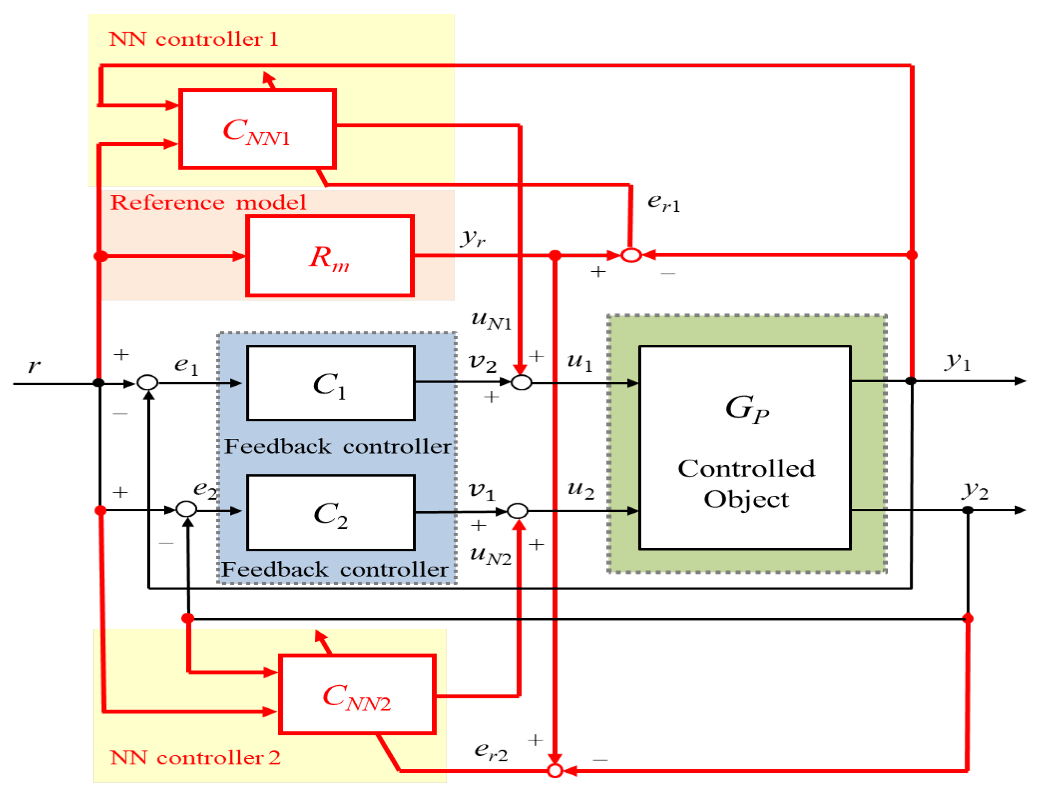
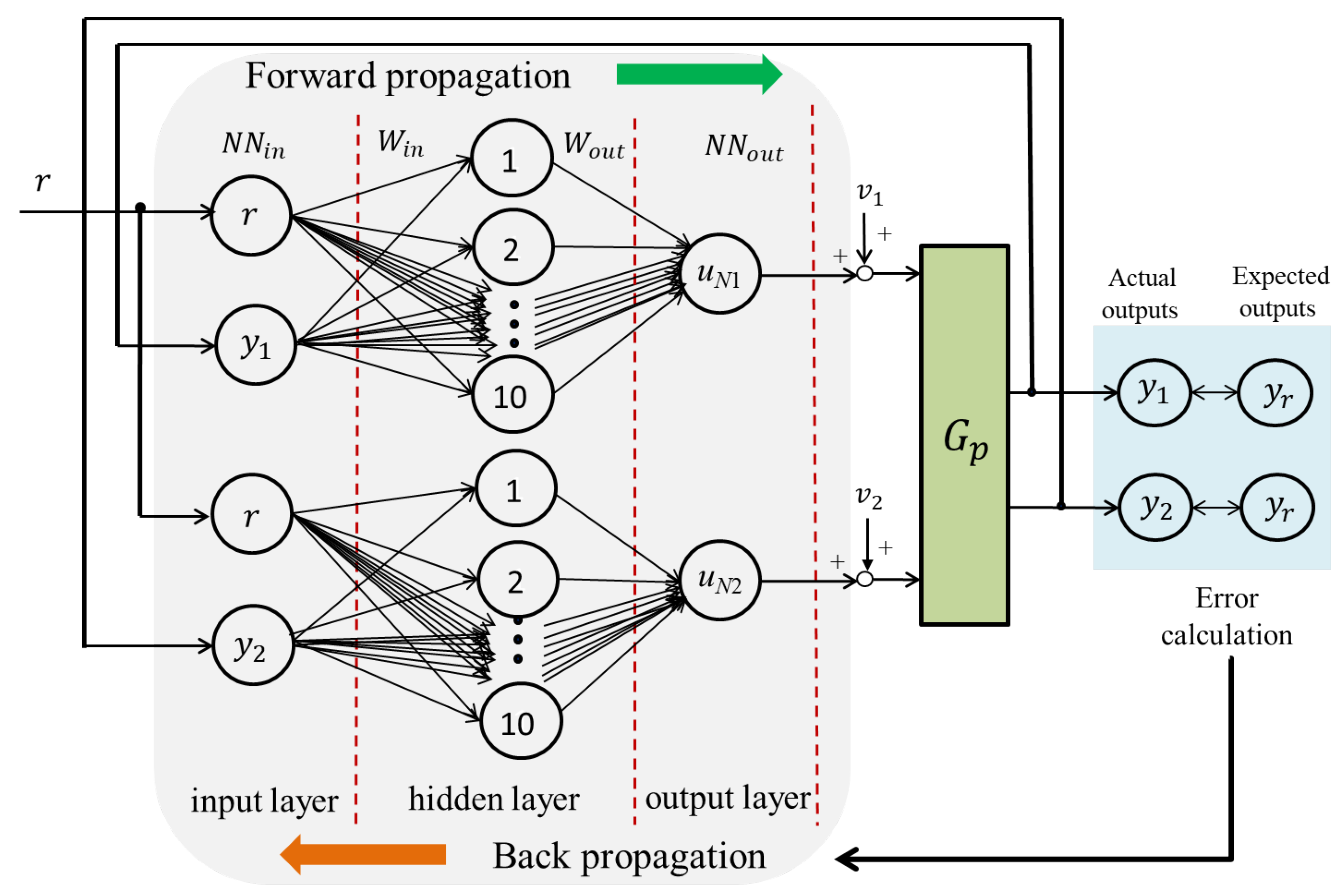
This section describes the configuration of the proposed reference-model-based NN control method in the MIMO control system. In this paper, the MIMO system is simplified as a two-input two-output (2I2O) model. The block diagram of the proposed temperature control system is shown in Figure 1.

As shown in Figure 1, the temperature controller consists of two feedback controllers $C_1$ and $C_2$, a reference model $R_m$, and two neural network controllers $C_{NN1}$ and $C_{NN2}$. Here, r is the reference of the system, and $y_1$ and $y_2$ indicate the actual outputs of two channels. $v_1$ and $v_2$ are the outputs of two feedback controllers $C_1$ and $C_2$, respectively. $u_{N1}$ and $u_{N2}$ indicate the outputs of $C_{NN1}$ and $C_{NN2}$, respectively. Thus, the control inputs of the two channels can be respectively indicated by $u_1$ and $u_2$ which can be expressed as the sum of the outputs of the NN controllers and I-PD controllers. $y_1$ and $y_2$ represent the inputs and outputs of the 2I2O controlled object, respectively. Due to the control object of each channel being a plant with a time delay, the reference model $R_m$ can be appropriately designed to provide the ideal temperature output with the same time delay which is the maximum time delay of two channels in the MIMO system. $e_{r1}$ and $e_{r2}$ are the errors between the outputs of the system and output of the reference model, respectively, which are the teaching signal for NN. The NN controller adjusts control inputs to compensate for the difference between the reference model output and each channel output. The explanation of the control system is divided into four main parts.

2.1. MIMO Controlled Objects with Strong Coupling Effects

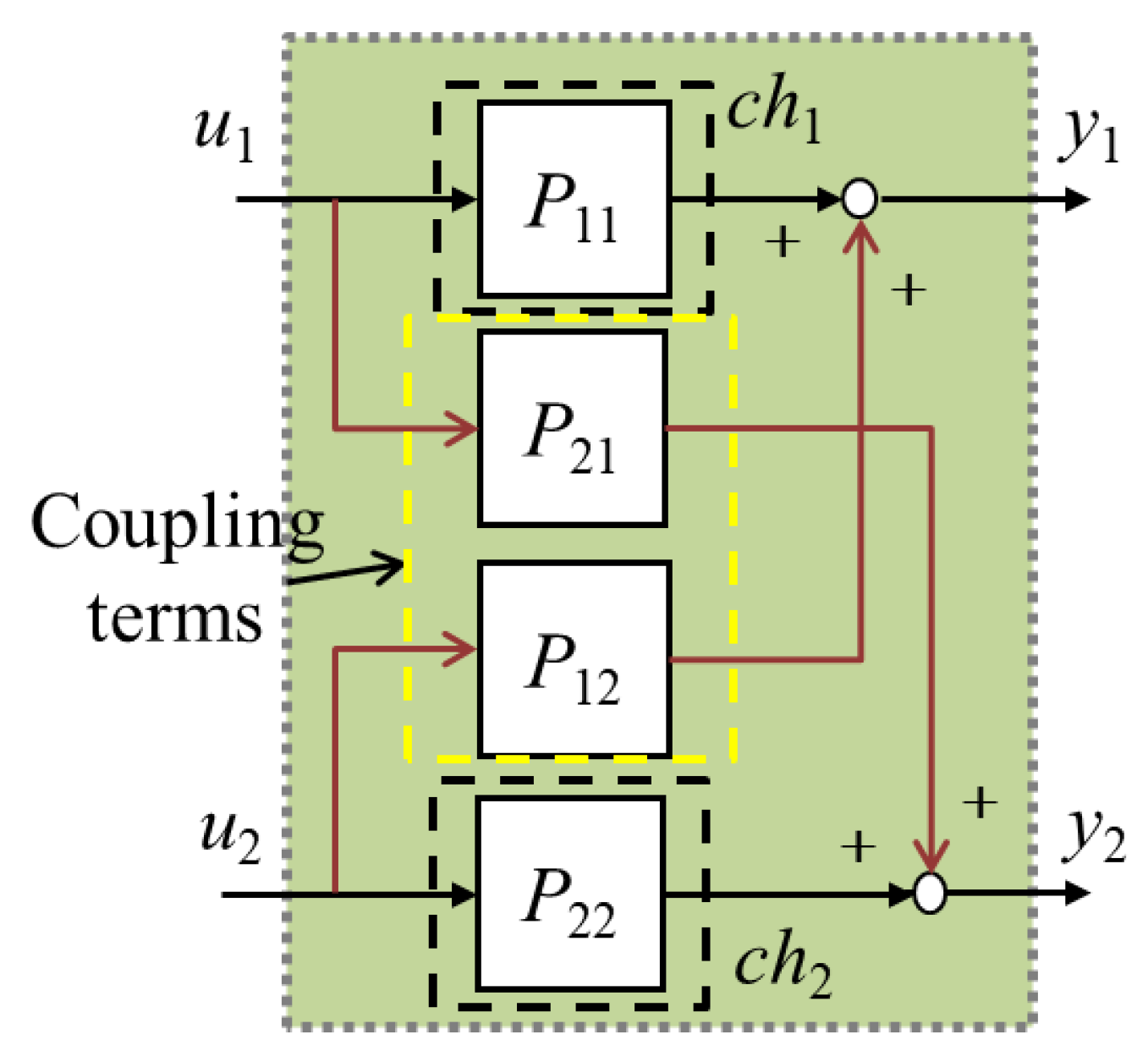
The control system is designed based on the MIMO temperature system with a strong coupling influence, the schematic block diagram of the coupled system is shown in Figure 2, where u${}_1$ and u${}_2$ are defined as the inputs of channel ch1 and channel ch2, respectively. In addition, y${}_1$ and y${}_2$ indicate the output of ch1 and ch2, respectively. 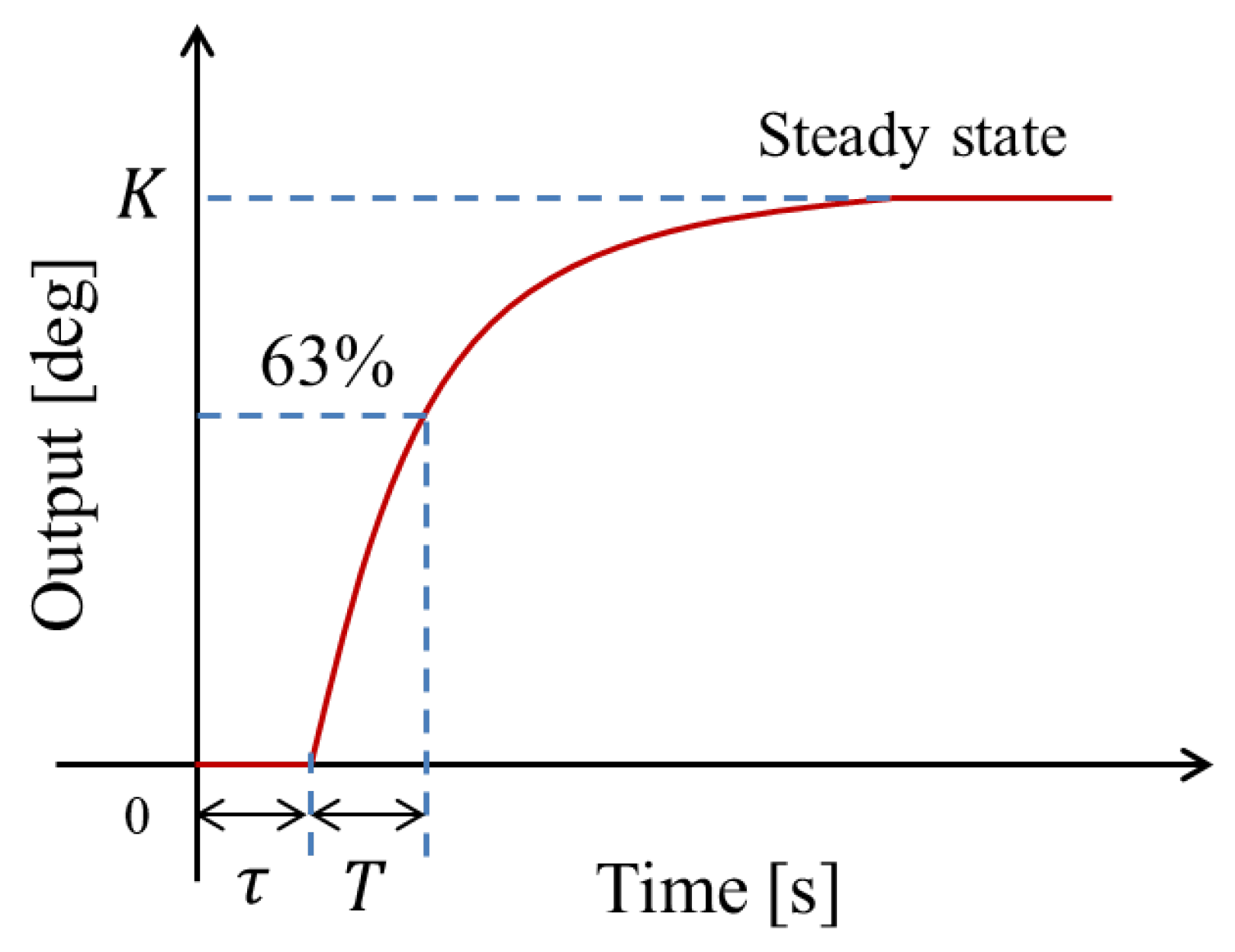The coupling terms between the two channels are obtained as P${}_{21}$ and P${}_{12}$, respectively. In this proposal, the controlled objects can be defined as a first-order plus time delay (FOPTD) system expressed as Equation (1) [29]. The step response characteristics of the controlled object is shown in Figure 3, where $\tau$ is time delay, K is the steady-state gain, and T is the time constant.

$$P\left(s\right)=\frac{K}{Ts+1}{e}^{-\tau s}$$

(1)

2.2. Conventional I-PD Controller

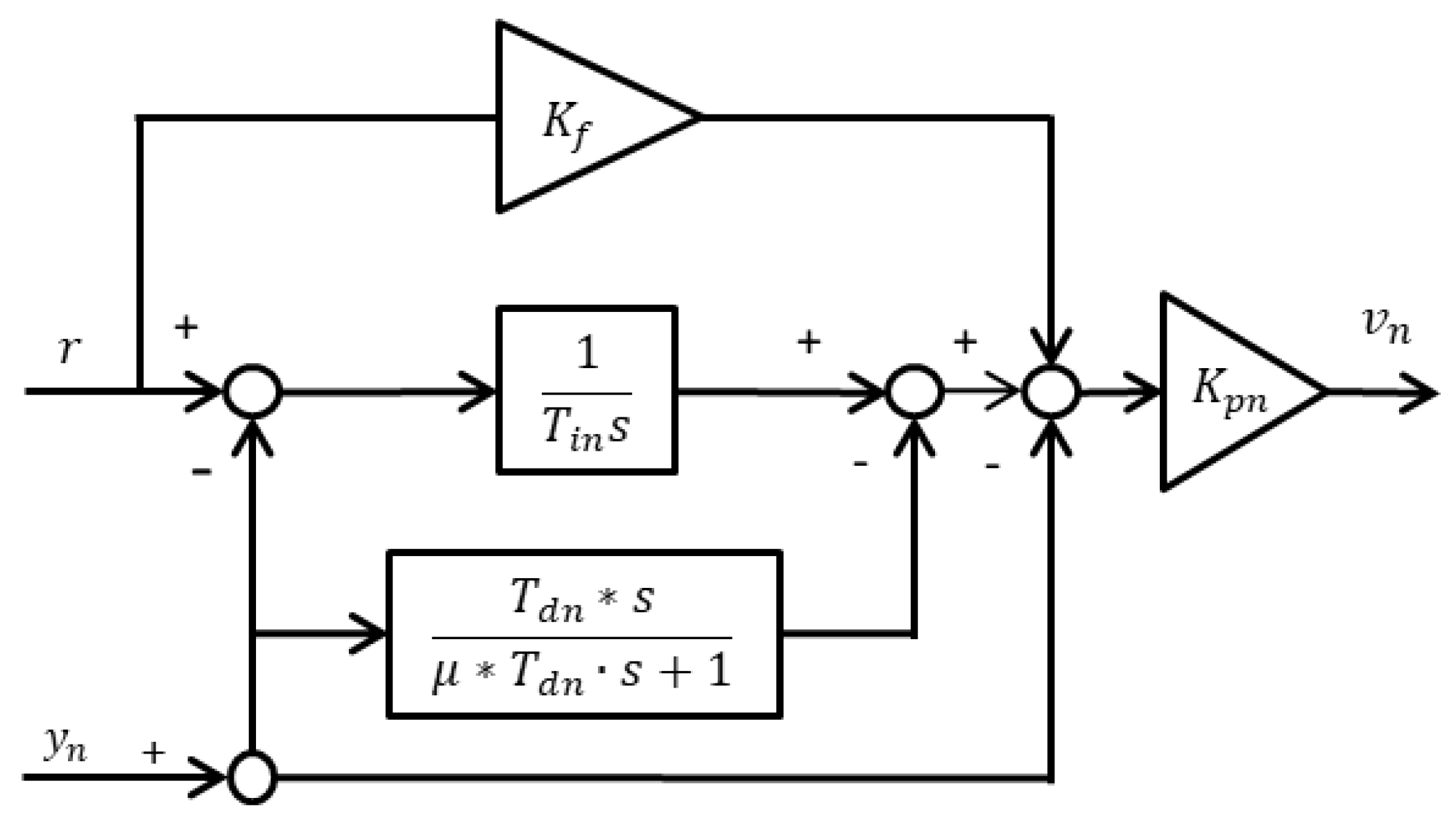
Considering that the NN controller needs time to train its parameters for getting expected outputs, it will mainly act after training. Thus, the conventional I-PD controllers as the feedback controllers are designed for each channel to eliminate the proportional and derivative kick appeared during the set-point change and reduce the undesirable overshoot of the controlled variable [30]. The block diagram of the conventional I-PD controller is shown in Figure 4. For each I-PD controller parameters of the system, $K_{pn}$ is the proportional gain and $T_{in}$ is the integral time constant. $T_{dn}$ represents the derivative time constant, where $n=1,2$. They are related to the plant parameters (K, T, and $\tau$) as described above. In addition, $\mu$ represents the low-pass filter gain of the derivative term for reducing the high-frequency gain and noise. The feed-forward gain $K_f$ is added to decide the system response speed ($K_f=0$: slow; $K_f=1$: fast).

For the industrial PID controller tuning, Ziegler–Nichols tuning rules are recognized and widely applied in actual control systems. The robustness and stability of the controllers are ensured. The parameters of two I-PD controllers $C_1$ and $C_2$ are calculated based on this tuning rule as Equations (2)–(4).

$$T_{i1}=2{\tau }_{11};T_{i2}=2{\tau }_{22}$$

(2)

$$T_{d1}=0.5{\tau }_{11};T_{d2}=0.5{\tau }_{22}$$

(3)

$$K_{p_1}=\frac{1.2T_{11}}{K_{11}\ast {\tau }_{11}};K_{p_2}=\frac{1.2T_{22}}{K_{22}\ast {\tau }_{22}}.$$

(4)

2.3. Multi-Layer NN Controller

In order to realize the uniform temperature of different channels, a multi-layer NN controller is introduced into each channel of the control system for the reference model output tracking. In the proposed system, each NN controller has one input layer with two neurons, one hidden layer with 10 neurons, and one output layer with one neuron. Thus, the structure of each multi-layer NN controller can be described as 2-10-1. Figure 5 illustrates the multi-layer neural network controllers.

In this system, the reference value of the system r and $y_1$ (the output of ch1) are set as the input signals of the NN controller1, r and $y_2$ (the output of ch2) are set as the input signals of the NN controller2. For each controller, two inputs are transmitted in the forward direction through the network. The composition of the learning process of the network is by forward propagation and back propagation [31]. Neural network calculates and store intermediate variables from the input signals to the output signals, which is expressed as Equation (5):

$$N{N}_{out}=f(W_{out}\ast f(W_{in}\ast N{N}_{in}+b_1)+b_2).$$

(5)

For each NN controller, $N{N}_{in}$ is the input vector and $N{N}_{out}$ is the output vector. $W_{in}$ and $W_{out}$ are connection weights of neurons. $b_1$ is the bias of the hidden layer neurons, $b_2$ is the bias of the output layer neurons, and $f(\ast )$ is the activation function.

For training the network, the back propagation algorithm is used to update the weights and biases. Through this process, each NN controller constantly adjust its outputs $u_{N1}$ and $u_{N2}$ for achieving the minimum error between the reference model output and actual outputs of two channels in this system. Considering one of the NN controllers, a neuron in the output layer is called neuron j (here $j=1$). The error at the output of the neuron j for nth iteration is defined by Equation (6). In the backward process, weights on the connections between all layers will be updated to minimize the error between target and output until the optimum weights are found [32]. Therefore, the total error is the sum of $e_j$ for all neurons in the output layer, as given in Equation (7):

$$e_j\left(n\right)=y_r\left(n\right)-y_j\left(n\right)$$

(6)

$$\epsilon \left(n\right)=\frac{1}{2}\sum _j{e}_j^2\left(n\right)$$

(7)

where the reference model output $y_r$ is the expected output for neuron j and $y_j\left(n\right)$ is the actual outputs of two channels. The output for the neuron j can be expressed as Equation (8), where $k=10$ is the number of inputs from the hidden layer. Here, $W_{j0}$ equals the bias $b_j$ applied to the neuron j:

$$y_j\left(n\right)=f(\sum _{i=0}^k{W}_{ji}\left(n\right)y_i\left(n\right)).$$

(8)

The connection weights of the neuron j are updated by the chain rule, and can be expressed in Equation (9), where ${\delta }_j\left(n\right)$ represents the local gradient of neuron j, given in Equation (10):

$$\frac{\partial \epsilon \left(n\right)}{\partial W_{ji}\left(n\right)}={\delta }_j\left(n\right)y_i\left(n\right)$$

(9)

$${\delta }_j\left(n\right)=-e_j\left(n\right)f^{\prime }(\sum _{i=0}^k{W}_{ji}\left(n\right)y_i\left(n\right)).$$

(10)

Therefore, the weight $w_{ij}$ is updated by adopting the gradient descent, expressed as Equation (11). The correction $\Delta W_{ij}$ ensures $w_{ij}$ changes in a way that always decreases the error, given in Equation (12), where $\alpha$ represents the learning rate of the back propagation:

$$W_{ji}(n+1)=W_{ji}\left(n\right)+\Delta W_{ij}\left(n\right)$$

(11)

$$\Delta W_{ij}\left(n\right)=-\alpha \frac{\partial \epsilon \left(n\right)}{\partial W_{ji}\left(n\right)}.$$

(12)

The neuron bias connection for the neuron j is adjusted by ${\delta }_j\left(n\right)$ during training, as given in Equation (13), where $\beta$ is the training gain of the bias:

$$b_j(n+1)=b_j\left(n\right)+\beta {\delta }_j\left(n\right).$$

(13)

In order to accelerate the training speed and solve the vanishing problem in the NN controller, the rectified linear unit (ReLU): $f\left(x\right)=max(0,x)$ is used as the activation function [33]. The derivative of the function is given in Equation (14):

$$f^{{}^{\prime }}\left(x\right)=\left\{\begin{array}{cc}1,\hfill & x\ge 0\hfill \\ 0,\hfill & x<0\hfill \end{array}\right.$$

(14)

2.4. Reference Model

In the reference-model-based NN control structure, the teaching signal of each NN controller is provided by errors between the reference model output and real plant output. It also helps to prevent over learning of the NN controller.

For the controller design, time delays in the dynamic systems can be approximated by rational transfer functions. The exponential function can be defined as follows [34]:

$$e^x\approx \underset{n\to \infty }{lim}\frac{1}{{(\frac{x}{n}+1)}^n}.$$

(15)

In order to save memory and consider trade-off between accuracy and calculation burden, the time delay $e^{-\tau s}$ which is written as $1/e^{\tau s}$ can be described as the second-order rational approximation in Equation (16):

$$e^{-\tau s}\approx \frac{1}{{(\frac{\tau s}{2}+1)}^2}.$$

(16)

Then the reference model with time delay can be expressed as Equation (17). Here, $\tau$ and T are delay time and the time constant of the reference model, which are set based on the real system model. It is designed to provide the ideal temperature output with the same time delay $\tau$ which is the maximum time delay of channels in the MIMO system. In addition, the time constant T of the reference model is the smaller time constant in the identified system model. The gain $P_{RM}$ value of 0.01 is added to the plant time constant T for improving the transient response speed of the system:

$$R_m\left(s\right)=\frac{1}{T·P_{RM}·s+1}\ast \frac{1}{{(\frac{\tau s}{2}+1)}^2}.$$

(17)

3. Simulation Results

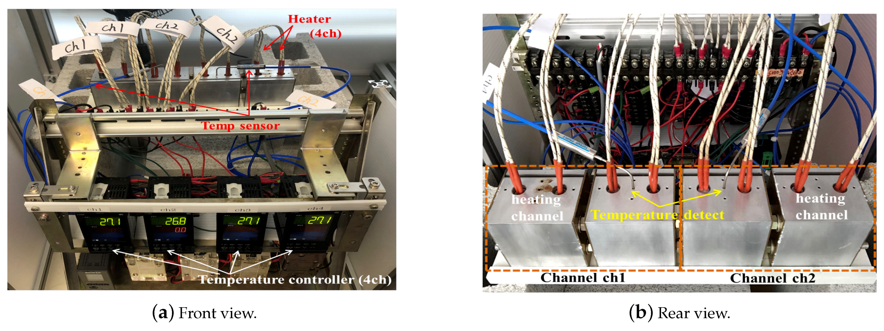
To verify the efficiency of the proposed control method, the control object is based on a real temperature control system. Figure 6 shows the experimental setup for the multi-input multi-output temperature system with strong coupling effects and large time delays.

3.1. Experimental Setup and System Identification

This system has four coupled aluminum blocks, the size being 60 × 60 × 50 (mm). As shown in Figure 6b, they are arranged in line with the same separation distance by nuts, forming a two-input two-output system with strong coupling and large time delays. The left two blocks as a whole are channel ch1 and the right two blocks as a whole are channel ch2. Channel ch1 and channel ch2 have two heaters of 150 W (Cartridge Heater, type G2A56, WATLOW, Chiyoda, Japan) and the temperature sensor (K type thermocouple, RKC, Tokyo, Japan), respectively. The temperature sensor transforms the temperature (0–400 ${}^{\circ }$C) into the output voltage (0–10 VDC). They are placed inside of holes with a depth of 30 [mm] (close to the inner center of aluminum blocks). The heaters are controlled by the solid-state relay (SSR, type G3PE-245BL, Omorn, Tokyo, Japan), which is driven by the pulse width modulation (PWM). The temperature is controlled by changing the duty ratio of the PWM signals. A digital signal processor (DSP, DS1104 R&D Controller Board, dSPACE Japan, Tokyo, Japan) is implemented as the temperature controller. The sampling time is set as 0.1 [s]. Although the SSR is a nonlinear element for the relay based on the PWM duty signal, it can be considered as the gain if the switching frequency of the relay is sufficiently large in comparison to the control bandwidth of the controlled object. In our system, the control bandwidth is $\frac{1}{2\pi \ast P_{RM}\ast T}=0.0064$ [Hz] ($P_{RM}\ast T$ is the reference model time constant), while the PWM frequency is 10 [Hz]. Therefore, SSR can be handled as a linear factor.

The step signal (20% PWM duty cycle) is added to ch1 and ch2, in order. The heaters of the ch1 and heaters of ch2 are actuated, respectively. The ambient temperature during the performed identification experiments was 28 ${}^{\circ }$C. The controlled object of the temperature control system is identified from the input-output(step response) measured data. The ARX (auto-regressive with eXogenous) model based on the least-squares criterion is applied to estimate the system transfer functions in MATLAB. The following Equation (18) shows the form of the ARX model, where $u\left(k\right)$ is the system inputs, $y\left(k\right)$ is the system outputs, $n_k$ is the system delay, and $e\left(k\right)$ is the system disturbance:

$$A\left(q\right)y\left(k\right)=B\left(q\right)u(k-n_k)+e\left(k\right).$$

(18)

In Equation (18), A(q) and B(q) are given as follows:

$$A\left(q\right)=1+a_1{q}^{-1}+\cdots +a_{n_a}{q}^{-n_a}$$

(19)

$$B\left(q\right)=b_1{q}^{-1-n_k}+\cdots +b_{n_b}{q}^{-n_b-n_k}$$

(20)

where $n_a$ and $n_b$ are the orders of polynomial A(q) and B(q), respectively. The parameters of A(q) and B(q) are determined using the least squares method that minimizes the quadratic prediction error criteria. In MATLAB, the identified discrete-time model is transformed into the continuous-time model and model order is reduced by balanced realization, obtaining the identified system model in the form of first-order plus time delay [35,36]. The performance parameter used for validating the identified model is the percentage of fit as the following expression (21), where $y\left(k\right)$ is the actual output, $\widehat{y}\left(k\right)$ is the model output, and $\overline{y}\left(k\right)$ is the mean of the actual output:

$$Fit(\%)=(1-\frac{\sqrt{{\sum }_{k=1}^N{[\widehat{y}\left(k\right)-y\left(k\right)]}^2}}{\sqrt{{\sum }_{k=1}^N{[y\left(k\right)-\overline{y}\left(k\right)]}^2}})\times 100\%.$$

(21)

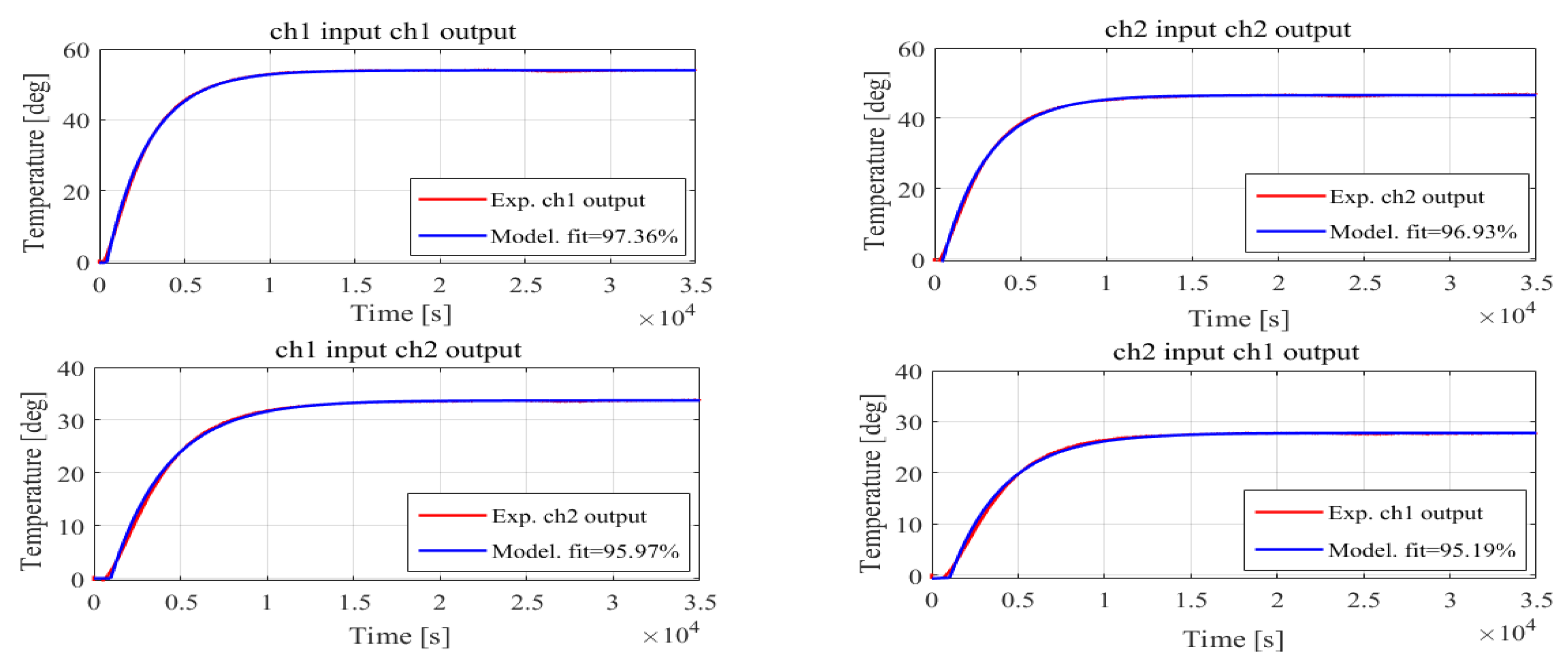
The identification results of the coupling terms are shown in Figure 7 and the estimation fit in results shows that the accuracy of the estimated model is above 95%.

Thus, the identification results can be finalized as (22). The system controller parameter design, system simulation, and experiments are all based on the identified plant transfer functions:

$$G_p\left(s\right)=\left[\begin{array}{cc}{P}_{11}& P_{12}\\ P_{21}& P_{22}\end{array}\right]=\left[\begin{array}{cc}\frac{2.7502}{2482.4s+1}{e}^{-431s}& \frac{1.4614}{3085.1s+1}{e}^{-1042s}\\ \frac{1.7352}{3195.9s+1}{e}^{-973s}& \frac{2.3937}{2588.6s+1}{e}^{-464s}\end{array}\right].$$

(22)

3.2. Simulation Results

According to the identified system model, the gains of two I-PD controllers are determined by the Ziegler–Nichols method, as described above. The gains of the I-PD controller ($C_1$) are $K_{p1}$ = 2.5146, $T_{i1}$ = 861.5, and $T_{d1}$ = 215.375. The gains of the I-PD controller ($C_2$) are $K_{p2}$ = 2.7968, $T_{i2}$ = 927.98, and $T_{d2}$ = 231.995. In addition, the reference model $R_m\left(s\right)$ is given as (23). Here, $P_{RM}$ is set as 0.01:

$$R_m\left(s\right)\approx \frac{1}{2482.4\ast 0.01\ast s+1}\ast \frac{1}{{(\frac{464s}{2}+1)}^2}.$$

(23)

The hyper-parameters of both NN controllers are initialized as follows: The learning rate $\alpha$ = $1\times {10}^{-10}$ and the bias training gain $\beta$ = $1\times {10}^{-5}$. They are determined via the try and error method. The initial biases of each layer are initialized as zero. The weights of the NN controller are initialized to small random values between $-1$ and 1.

The simulation is divided into two phases. In the first phase, setting the reference signal to 100 ${}^{\circ }$C, then the temperature of different channels increases from 0 ${}^{\circ }$C to 100 ${}^{\circ }$C. During this period, the neural network controller completes learning. Then, in the second phase, a repetitive step signal with an amplitude of 5 ${}^{\circ }$C is added to the reference signals periodically. The offset of the reference signal is 100 ${}^{\circ }$C. In one cycle, the temperature is controlled from 100 ${}^{\circ }$C to 105 ${}^{\circ }$C, then return to 100 ${}^{\circ }$C. After multiple cycles, the first step response and last step response results in both directions can be obtained. Here, the temperature from 100 ${}^{\circ }$C to 105 ${}^{\circ }$C is defined as the positive direction control and the temperature from 105 ${}^{\circ }$C to 100 ${}^{\circ }$C is defined as the negative direction control.

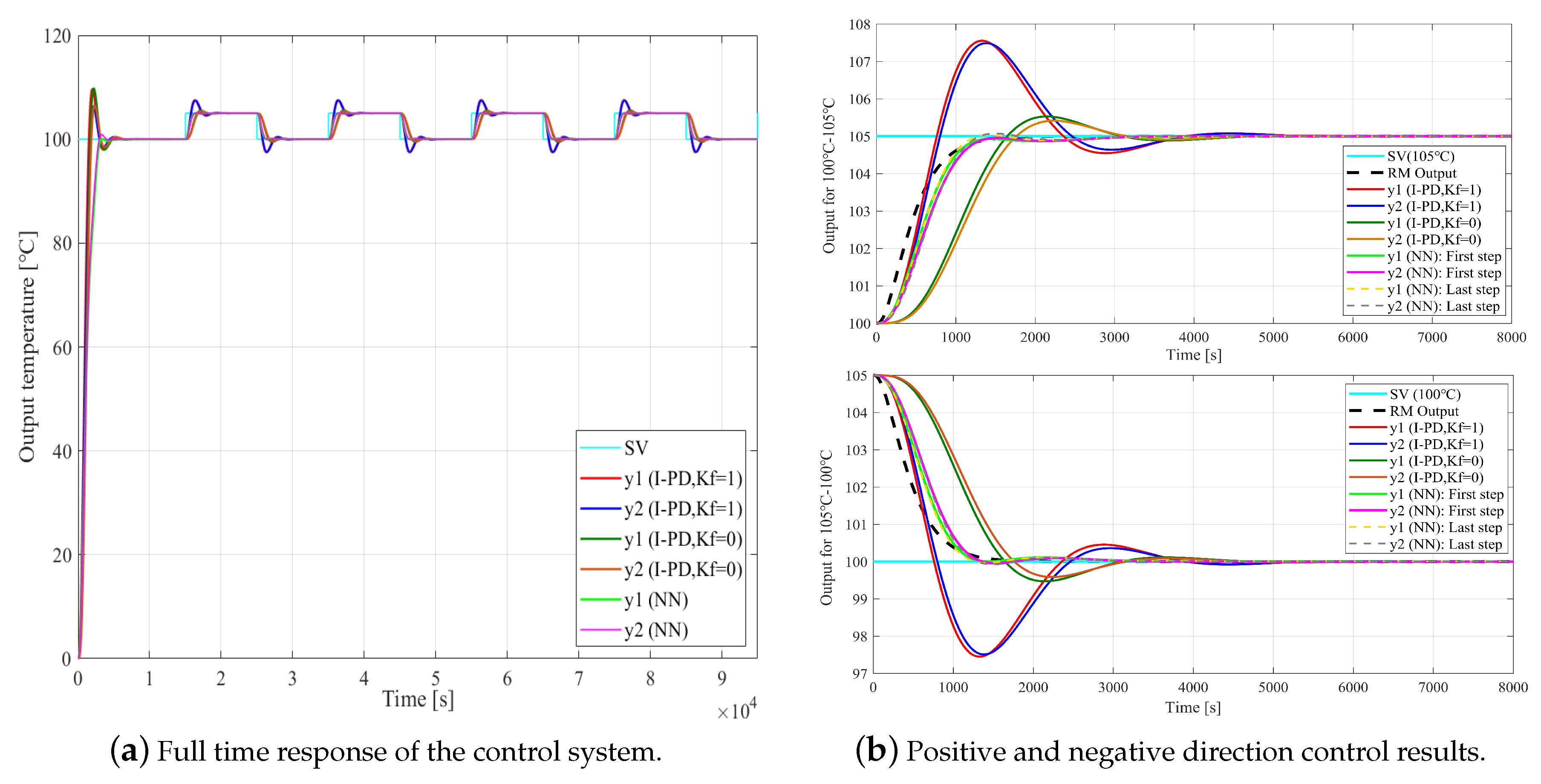
Figure 8a shows the full time response of the control system and (b) shows the results of positive direction control (from 100 ${}^{\circ }$C to 105 ${}^{\circ }$C) and negative direction control (from 105 ${}^{\circ }$C to 100 ${}^{\circ }$C) of the NN control system. From the NN control system results, the first step response is almost the same as the last response, meaning the learning of the NN control ends at the beginning of the first step. Thus, the NN controllers realize the quick-learning. These results are quantitatively compared with those obtained by the conventional I-PD control with different feed-forward gains $K_f=0$ (slow response) and $K_f=1$ (fast response). The step-response characteristics of systems are computed from the response data in MATLAB, the rise time of a response is defined as the change in time required for the response to rise from 10% to 90% of the desired steady-state response yfinal (here, 105 ${}^{\circ }$C and 100 ${}^{\circ }$C, respectively). Furthermore, the settling time is defined as the time required for the error between the time response y(t) and yfinal to fall below 5% of the yfinal. Percentage overshoot is also relative to yfinal.

In the positive direction, two channels of the proposed NN control system follow the reference model as much as possible. The rise time of ch1 and ch2 in the NN control system is 753.2 s and 787.9 s, respectively. Compared with that of the I-PD ($K_f=0$) control system, which is 931.2 s and 990.1 s, ch1 and ch2 has an improvement of 23.6% and 25.7%, respectively. Compared with that of the I-PD ($K_f=1$) system which is 459.2 s and 482.4 s, although the transient response of the I-PD ($K_f=1$) system is faster, the overshoots of two channels are 2.43 ${}^{\circ }$C and 2.37 ${}^{\circ }$C, which are about 48.6% and 47.5% of the reference value, respectively. The overshoots of two channels in the I-PD ($K_f=0$) system are 0.51 ${}^{\circ }$C and 0.4 ${}^{\circ }$C, which are about 10.1% and 8% of the reference value, respectively. By contrast, both overshoots of the proposed NN system outputs are zero.

In addition, the settling time of ch1 and ch2 in the NN control system is 2225.1 s and 2178.4 s. Compared with that of the I-PD ($K_f=1$) control system which is 3666.3 s and 3554.5 s, both channels have an improvement of about 42%. Compared with that of the I-PD ($K_f=0$) control system which is 3634.9 s and 3144.1 s, ch1 improved by 38% and ch2 improved by 31%, respectively. The NN control system was the fastest to reach stable state without overshoots. Simulation results for the temperature from 100 ${}^{\circ }$C to 105 ${}^{\circ }$C are presented in

Table 1. Comparison of simulation results for time response characteristics (100 ${}^{\circ }$C to 105 ${}^{\circ }$C).

100 ${}^{\circ }$C to 105 ${}^{\circ }$C	Ref	ch1 (${\mathit{K}}_{\mathit{f}}=1$)	ch2 (${\mathit{K}}_{\mathit{f}}=1$)	ch1 (${\mathit{K}}_{\mathit{f}}=0$)	ch2 (${\mathit{K}}_{\mathit{f}}=0$)	ch1 (NN)	ch2 (NN)
Rise Time (s)	780.7	459.2	482.4	931.2	990.1	753.2	787.9
Settling Time (s)	1378.2	3663.0	3554.5	3634.9	3144.1	2225.1	2178.4
Overshoot (%)	0	48.6	47.5	10.1	8.0	0	0

. The rise time and settling time reflect the transient response and steady-state response speed of the control systems, respectively.

In the negative direction, the temperature signal varies from 105 ${}^{\circ }$C to 100 ${}^{\circ }$C. Response characteristics of different control systems are compared and results are similar to the corresponding results in the positive direction. The rise time of ch1 and ch2 in the NN control system is 726.7 s and 772.2 s, respectively. Compared with that of the I-PD ($K_f=0$) control system, which is 931.2 s and 990.1 s, ch1 and ch2 has an improvement of 21.9% and 22%, respectively. Compared with that of the I-PD ($K_f=1$) system which is 459.2 s and 482.4 s, although the transient response of the I-PD ($K_f=1$) system is faster, the overshoots of two channels are 2.43 ${}^{\circ }$C and 2.37 ${}^{\circ }$C, which are about 48.6% and 47.5% of the reference value, respectively. The overshoots of the two channels in the I-PD ($K_f=0$) system are 0.51 ${}^{\circ }$C and 0.4 ${}^{\circ }$C, which are about 10.1% and 8% of the reference value, respectively. By contrast, both overshoots of the proposed NN system outputs are zero.

Additionally, the settling time of ch1 and ch2 in the I-PD ($K_f=0$) control system is 3689 s and 3135.5 s. In the NN control system, it is 2241.3 s and 2164.5 s, which has an improvement of 39% and 31%, respectively. Compared with that of the I-PD ($K_f=1$) control system which is 3669 s and 3553 s, the NN control system improved by 38.9% and 39%. From simulation results, different channels in the NN control system can quickly reach the stable state with no overshoot in contrast to the large overshoots of the I-PD control systems. Simulation results for temperature from 105 ${}^{\circ }$C to 100 ${}^{\circ }$C are presented in

Table 2. Comparison of simulation results for time response characteristics (105 ${}^{\circ }$C to 100 ${}^{\circ }$C).

105 ${}^{\circ }$C to 100 ${}^{\circ }$C	Ref	ch1 (${\mathit{K}}_{\mathit{f}}=1$)	ch2 (${\mathit{K}}_{\mathit{f}}=1$)	ch1 (${\mathit{K}}_{\mathit{f}}=0$)	ch2 (${\mathit{K}}_{\mathit{f}}=0$)	ch1 (NN)	ch2 (NN)
Rise Time (s)	780.7	459.2	482.4	931.2	990.1	726.7	772.2
Settling Time (s)	1378.2	3669.0	3552.0	3689.0	3135.5	2241.3	2164.5
Overshoot (%)	0	48.6	47.5	10.1	7.9	0	0

. These results show that the proposed NN control system has improved the temperature control efficiency in both directions.

Figure 9a,b, respectively show the temperature differences between ch1 and ch2 in positive and negative directions, using I-PD control with gains $K_f=1$, 0 and the proposed NN control.

In the positive direction, the maximum temperature difference of the I-PD control with gains $K_f=1$ and $K_f=0$ are 0.35 ${}^{\circ }$C and 0.31 ${}^{\circ }$C, about 7% and 6.2% of the reference temperature, respectively. The result of the proposed NN control system is 0.23 ${}^{\circ }$C, about 4.6% of the reference temperature. The maximum temperature difference of the NN control system is decreased by 2.4% and 1.6%, compared to results of I-PD ($K_f=0$) and I-PD ($K_f=1$) control systems. Meanwhile, the temperature difference of the NN control drops to 0 ${}^{\circ }$C in about 2400 s. The time has been shortened by 55% and 59% compared with the time for I-PD ($K_f=1$) and I-PD ($K_f=0$) control systems, which is about 5300 s and 5800 s.

In the negative direction, results are similar to those in the positive direction. The maximum absolute temperature difference of the NN control system and the I-PD control system with gains $K_f=1$ and $K_f=0$ are about 0.24 ${}^{\circ }$C, 0.34 ${}^{\circ }$C and 0.31 ${}^{\circ }$C, corresponding to 4.8%, 6.8%, and 6.2% of the reference value. The maximum temperature difference in the NN control system decreased by 1.4% and 1.6%, when compared to the results of I-PD ($K_f=0$) and I-PD ($K_f=1$) control systems. Meanwhile, the temperature difference of the NN control drops to 0 in about 2300 s. The time is shortened by 57% and 60% compared to that of I-PD ($K_f=1$) and I-PD ($K_f=0$) control systems, which is about 5400 s and 5700 s. From these simulation results, although the maximum temperature difference between ch1 and ch2 is not suppressed drastically, quick transient response and uniform temperature in different channels can be achieved.

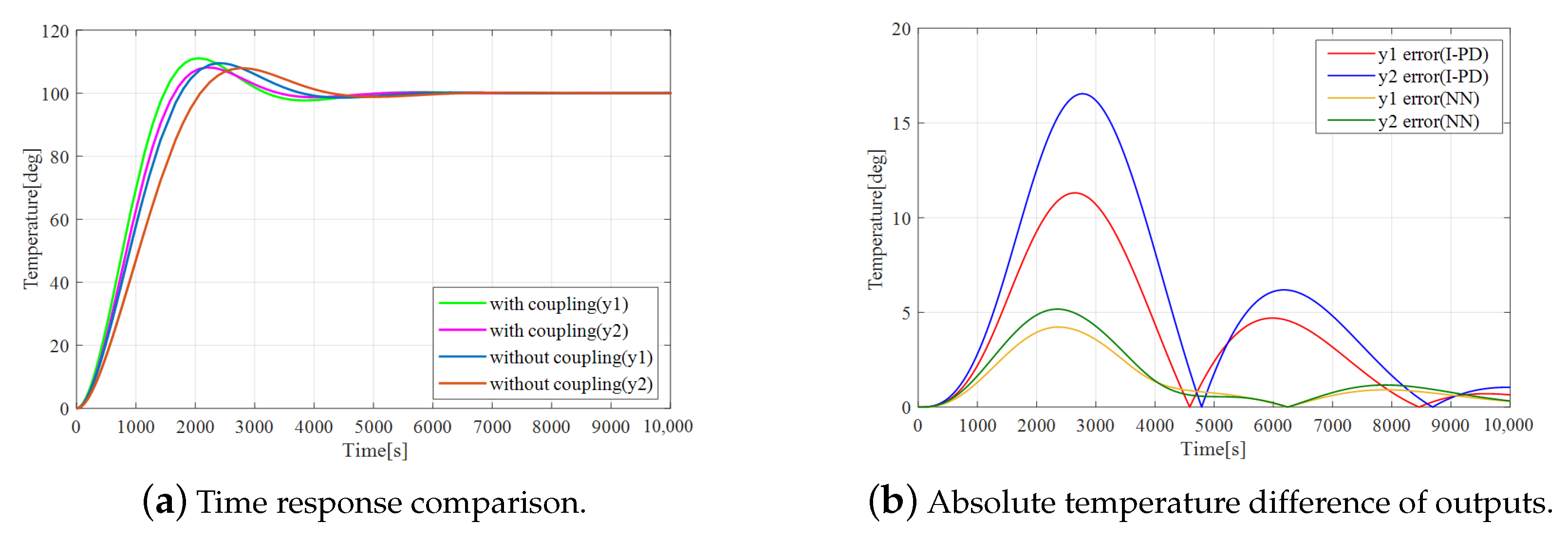
In order to analyze the influences of the coupling terms between different channels, the time response results of the I-PD ($K_f=1$) control system with coupling and without coupling effects are given in Figure 10, the reference signal is set to 100 ${}^{\circ }$C. The overshoots of the system with coupling terms become bigger, about 11.2% and 8.4% of the reference signal. The overshoots of the system without coupling terms are about 9.4% and 7.8%, respectively. In addition, a slight oscillation is enhanced in both outputs for the coupling effects. From absolute temperature differences of outputs between the control system with coupling effects and without coupling effects, both output temperature differences in the I-PD system are large, with maximum values of about 11.4 ${}^{\circ }$C and 16.6 ${}^{\circ }$C, respectively. The maximum errors of the NN control system are about 4.2 ${}^{\circ }$C and 5.1 ${}^{\circ }$C in output temperatures. The proposed NN control system can effectively weaken the coupling terms influences on the control system outputs.

4. Experimental Results

According to the identified system model introduced in the simulation, experiments with the proposed NN control method are carried out in the real temperature control system. The experimental setup is shown in Figure 6. Experimental conditions are as follows: The room temperature is set at 28 ${}^{\circ }$C, sampling period is 0.1 s, controller sampling bit is 12 bits and the sensor resolution is 0.1 ${}^{\circ }$C. In experiments, the reference temperature is first set to 100 ${}^{\circ }$C, the temperature of two channels is controlled from the room temperature to 100 ${}^{\circ }$C. Then a repetitive step signal with amplitude of 5 ${}^{\circ }$C is added to the reference periodically. The temperature is controlled from 100 ${}^{\circ }$C to 105 ${}^{\circ }$C, then return to 100 ${}^{\circ }$C. This process is repeated many times. The temperature increases from the room temperature to 100 ${}^{\circ }$C, defined as the learning period of the NN controller, and the temperature from 100 ${}^{\circ }$C to 105 ${}^{\circ }$C and from 105 ${}^{\circ }$C to 100 ${}^{\circ }$C are the control results of the NN control system. For NN learning in the first step, we roughly estimated [$u_{N1}$, $y_1$, $e_{r1}$, $u_{N2}$, $y_2$, $e_{r2}$] × 100,000 steps (sampling time 0.1 s) = $6.0\times {10}^5$ data is required to complete the learning. For testing the learned NN, one sequence of the step response is needed. Therefore, the same data number is required. Similarly, in the simulation, to verify the control performance of the proposed method, results are compared with those of the I-PD control with gains $K_f=1$ (slow) and $K_f=0$ (fast).

Figure 11a shows the results for full time response of the control system, and (b) shows the results for the temperature changes in positive and negative directions. As shown in Figure 11b, the I-PD control system with gain $K_f=1$ has the fastest transient response speed, but is the slowest to reach the steady state in both directions. For the I-PD control system with gain $K_f=0$, both the transient response and steady-state response are slower than the NN control system in both directions.

The time response characteristics of controlled systems are extracted from positive direction and negative direction response data in MATLAB. The response data is loaded, which is an array of response data y and corresponding time vector t. The 2nd-order butterworth digital low-pass filter with a cutoff frequency of 0.05 Hz (sampling frequency is 10 Hz) is applied to eliminate as much of the noise in the data as possible. The response characteristics were calculated from these data using the command “S = stepinfo(y, t, yfinal)” in MATLAB. Considering the noise in the data, the last value in y may not have the true steady-state response value. Therefore, the steady-state value (yfinal) should be set as 105 and 100 in the positive and negative direction control, respectively. The response characteristics of controlled systems such as rise time, settling time, and overshoot can be obtained.

In the positive direction, the rise time of ch1 and ch2 in the I-PD ($K_f=0$) control system is 947.2 s and 973.1 s, in the NN control system, it is 812.4 s and 820.6 s, which improved by 14.2% and 15.7%. The settling time of ch1 and ch2 in the I-PD ($K_f=0$) control system is 3414.2 s and 3217.9 s, and the NN control system had an improvement of 35.1% and 31.5%, which is 2217.3 s and 2204.8 s, respectively. In the I-PD ($K_f=1$) control system, the settling time of ch1 and ch2 is 3824.3 s and 3718.6 s. By comparison, the NN control system improved by 42% and 40.7%. In addition, the overshoots of ch1 and ch2 in the I-PD ($K_f=1$) control system are 2.01 ${}^{\circ }$C and 1.92 ${}^{\circ }$C, corresponding to 40.1% and 38.4% of the reference. The overshoots of ch1 and ch2 in the I-PD ($K_f=0$) control system are about 0.69 ${}^{\circ }$C and 0.53 ${}^{\circ }$C, corresponding to 13.9% and 10.5% of the reference. In the NN control system, the overshoot of ch1 and ch2 are about 0.06 ${}^{\circ }$C and 0.08 ${}^{\circ }$C, corresponding to 1.3% and 1.7% of the reference, much smaller than those in the I-PD control systems.

In the negative direction, similar results can be obtained. The rise time of ch1 and ch2 in the I-PD ($K_f=0$) control system is 1027.3 s and 1093.4 s, in the NN control system is 877.3 s and 893.7 s, which has been improved by 14.6% and 18.3%. The settling time of ch1 and ch2 in the I-PD ($K_f=0$) control system is 3492.7 s and 3325.1 s, the NN control system has an improvement of 38.6% and 37%, which is 2145.6 s and 2093.2 s, respectively. In the I-PD ($K_f=1$) control system, the settling time of ch1 and ch2 is 3862.5 s and 3870.4 s. By comparison, the NN control system improved by 44.5% and 45.9%, respectively. In addition, the overshoots of ch1 and ch2 in the I-PD ($K_f=1$) control system are about 2.14 ${}^{\circ }$C and 2.07 ${}^{\circ }$C, corresponding to 42.7% and 41.4% of the reference. The overshoots in the I-PD ($K_f=0$) control system are 0.62 ${}^{\circ }$C and 0.48 ${}^{\circ }$C, corresponding to 12.3% and 9.7% of the reference. In the NN control system, the overshoots of ch1 and ch2 are about 0.11 ${}^{\circ }$C and 0.12 ${}^{\circ }$C, which are 2.1% and 2.5% of the reference. The overshoots in both directions are much smaller than the results of the I-PD control systems. Two channels can track the reference model output, realizing a quick and stable response to temperature signals. Comparing experimental results of the system response in Figure 11 with the simulation results in Figure 8, the discrepancy between the real system performance and simulation within 5% either settling time or overshoot, e.g., the errors of the NN system for the positive direction are about 2.3% and 1.7% in settling time and 1.3% and 1.7% in overshoot, respectively, the negative direction results are about 4.3% and 3.3% in settling time and 2.1% and 2.5% in overshoot. The corresponding errors of the I-PD control systems are slightly larger than 5%, e.g., the errors of the I-PD ($K_f=0$) system for the negative direction are about 5.3% and 5.7% in settling time, respectively, the I-PD ($K_f=1$) system errors are about 5.1% and 8.2%. Although the errors of rise time are about 10% in both directions, considering the difference between different channels is almost negligible, results are acceptable. These results show a good agreement between simulated and experimental results.

For comparison, the response characteristics of different control systems in positive and negative directions are listed in

Table 3. Comparison of experimental results for time response characteristics (100 ${}^{\circ }$C to 105 ${}^{\circ }$C).

Characteristics	Ref	CH1 (${\mathit{K}}_{\mathit{f}}=1$)	CH2 (${\mathit{K}}_{\mathit{f}}=1$)	CH1 (${\mathit{K}}_{\mathit{f}}=0$)	CH2 (${\mathit{K}}_{\mathit{f}}=0$)	CH1 (NN)	CH2 (NN)
Rise Time (s)	780.7	534.9 (14.1%)	557.6 (13.4%)	947.2 (1.7%)	973.1 (1.7%)	812.4 (11.6%)	820.6 (4.1%)
SettlingTime 5% (s)	1378.2	3824.3 (4.2%)	3718.6 (4.4%)	3414.2 (6.1%)	3217.9 (2.3%)	2217.3 (2.3%)	2204.8 (1.7%)
Overshoot $(\%)$	0	40.1 (4.8%)	38.4 (3.4%)	13.9 (3.9%)	10.5 (2.5%)	1.3 (1.3%)	1.7 (1.7%)

and

Table 4. Comparison of experimental results for time response characteristics (105 ${}^{\circ }$C to 100 ${}^{\circ }$C).

Characteristics	Ref	CH1 (${\mathit{K}}_{\mathit{f}}=1$)	CH2 (${\mathit{K}}_{\mathit{f}}=1$)	CH1 (${\mathit{K}}_{\mathit{f}}=0$)	CH2 (${\mathit{K}}_{\mathit{f}}=0$)	CH1 (NN)	CH2 (NN)
Rise Time (s)	780.7	519.1 (11.5%)	535.5 (9.8%)	1027.3 (9.3%)	1093.4 (9.4%)	877.3 (17.1%)	893.7 (13.6%)
SettlingTime 5% (s)	1378.2	3862.5 (5.1%)	3870.4 (8.2%)	3492.7 (5.3%)	3325.1 (5.7%)	2145.6 (4.3%)	2093.2 (3.3%)
Overshoot $(\%)$	0	42.7 (5.9%)	41.4 (6.1%)	12.3 (2.2%)	9.7 (1.8%)	2.1 (2.1%)	2.5 (2.5%)

, respectively. The percentage differences between the experimental results and simulation results are also given in both tables. From the above experimental results, it is seen that the proposed NN control gives great improvement in the performance of the temperature system.

Figure 12a,b show the curves of temperature differences between the outputs of ch1 and ch2 in positive and negative directions, respectively. In the positive direction, the maximum temperature differences of the I-PD ($K_f=1$), I-PD ($K_f=0$), and NN control are 0.39 ${}^{\circ }$C, 0.43 ${}^{\circ }$C, and 0.15 ${}^{\circ }$C, which correspond to 6.4%, 9.4%, and 3.8% of the reference value, respectively. In addition, the time for the temperature difference drops to 0 ${}^{\circ }$C is about 3900 s, 3600 s, and 2300 s. The NN control system has an improvement of 41% and 36% compared to the I-PD ($K_f=1$) and I-PD ($K_f=0$) control system, respectively. As illustrated in Figure 12a, the temperature difference of the NN control system can be suppressed by the proposed method.

Similarly, in the negative direction, the maximum absolute temperature differences of the I-PD ($K_f=1$), I-PD ($K_f=0$), and NN control systems are 0.24 ${}^{\circ }$C, 0.25 ${}^{\circ }$C, and 0.14 ${}^{\circ }$C, corresponding to 4.8%, 5%, and 2.8% of the reference value. Moreover, the time for the temperature difference drops to 0 ${}^{\circ }$C is about 4400 s, 4100 s, and 3300 s, respectively. The NN control system has an improvement of 25% and 20% compared to the I-PD ($K_f=1$) and I-PD ($K_f=0$) control system, respectively. From these results, it was observed that the rapid uniform temperature response could be achieved in both transient state and steady state. The proposed control method improved the performance of the multi-input multi-output temperature system.

5. Conclusions

In this paper, to improve transient response and realize the temperature uniformity in the multi-input multi-output temperature system with strong coupling effects, a reference-model-based neural network control method was proposed. In order to confirm the effectiveness of the proposed method, the proposed NN method was applied to a real MIMO temperature control system. Simulation and experiments were carried out, respectively. Both simulation results and experimental results were quantitatively compared with those of the I-PD control systems. The improvement of the transient response was achieved from the above experimental results, e.g., 42% and 40.7% improvements of two channels in settling time shortening compared to those of the traditional I-PD ($K_f=1$) control system. In addition, the overshoots of different channels decreased by about 40% in both directions. The temperature uniformity of the MIMO system was achieved, e.g., in the positive direction, the temperature differences between two channels were reduced in more than half of those in the I-PD ($K_f=1$) and I-PD ($K_f=0$) control system. The temperature differences quickly went down to zero, with about 41% and 36% improvements in time compared to the I-PD control systems, respectively. These results show that the proposed NN control method improved the transient response and overshoot of the multi-input multi-output temperature system and realized the temperature uniformity of different channels in both transient state and steady state. The control effectiveness of the proposed method was successfully verified. For the NN control learning in the MIMO system, the selection of inputs and teaching signal is worth discussing in future study, e.g., the temperature difference between channels or derivative of difference can be added to inputs of the NN controller, thus it is possible to further improve the control performance.