A Closed-Loop Optimized System with CFD Data for Liquid Maldistribution Model

Abstract

For the simulation of a trickle-bed reactor (TBR) in coal and oil refining, modeling the liquid maldistribution of the gas-liquid distributor incurs enormous pre-processing work and bears a huge computational cost. A closed-loop optimized system with computational fluid dynamic (CFD) data is therefore proposed for the first time in this paper. A fast prediction model based on support vector regression (SVR) is developed to simplify the modeling of the liquid flow rate in TBRs. The model uses CFD simulation results to determine an optimized set of structural parameters for the gas-liquid distributor in TBRs. In order to obtain an accurate SVR model quickly, the particle swarm optimization (PSO) algorithm is employed to optimize the SVR parameters. Then, the structural parameters corresponding to the minimum liquid maldistribution factor are calculated using the response surface methodology (RSM) based on the hybrid PSO-SVR model. The CFD validation results show a good agreement with the values predicted by RSM, with liquid maldistribution factors of 0.159 and 0.162, respectively.

1. Introduction

Trickle-bed reactors (TBRs) are widely used in the chemical and oil industries. TBR efficiency relies on the good distribution of liquid feed over the catalyst bed cross section, so predicting liquid maldistribution is one of the critical issues in the efficient use of TBRs [1].

Several approaches have been developed to estimate liquid maldistribution. Cold model experiments are easy to implement and relatively simple to perform in laboratory-scale devices using a collector at the catalyst bed outlet. However, there is a possibility of flow redistribution at the exit of the bed [2,3,4]. To overcome this disadvantage, several groups have focuses on the use of tomographic measurements using photon attenuation (x-ray and γ-ray tomography), magnetic resonance imagining, and electric tomographic techniques, which provide more quantitative flow distribution information [5,6,7,8,9]. With the drawback of a high cost and unsafety, the performance of these techniques depends on the complexity of the reconstruction algorithms. Compared to these approaches, computational fluid dynamics (CFD) modeling has a relatively low cost and can simulate both realistic and ideal conditions [10,11,12,13,14]. However, a CFD simulation of the full geometry of a gas-liquid distributor may be time-consuming, depending on the domain size and the mesh number. Hence, a time-saving and reliable surrogate model is needed for CFD simulation.

The support vector regression (SVR) method is such a tool generally preferred for solving problems requiring high computational resources [15,16,17,18]. Recently, the applicability of SVR-based models in the field of chemical engineering has been well demonstrated. SVR models have already been applied in predicting the behavior of the gas–liquid interface area ($a$), $k_{La}$, and $k_{Ga}$ in TBRs [19] by Bansal et al. Jalalifar et al. proposed an SVR-particle swarm optimization (PSO) model and combined it with a CFD dataset to predict the best operating parameters of a pyrolysis reactor [20]. Zaidi used an SVR-based modeling technique to predict the cycle rates in a thermosiphon reboiler for different pure components with large variations in thermophysical properties and operating parameters [21].

In this paper, we propose a methodology for obtaining an optimized solution of the gas-liquid distributor in TBRs on the basis of limited data generated using CFD simulation in order to reduce the simulation time significantly. The flow chart for obtaining an optimized solution of the gas-liquid distributor in TBRs is shown in Figure 1. In step 1, CFD data is used as the input to develop an SVR model, and then PSO is used to accelerate the training speed to find the optimum parameter set for the SVR model. In step 2, the response surface method (RSM) is used to optimize the structure of the gas-liquid distributor according to the PSO-SVR model, and then the optimum structure is validated through CFD simulation.

The remainder of this paper is organized as follows. In Section 2, a hybrid modeling method of PSO-SVR based on CFD simulation data is proposed. In Section 3, the optimal structure of the gas-liquid distributor is obtained via RSM on the basis of the data from the PSO-SVR model. In Section 4, a comparison is carried out to evaluate the universality, accuracy, and rapidity of PSO-SVR model, and the optimization result is verified by CFD simulation. Finally, we draw conclusions and describe the future research directions in Section 5.

2. SVR Modeling Hybrid PSO Based on CFD Simulation

The present study aims to predict the liquid flow rate by training an SVR model of the TBR gas-liquid distributor with data obtained from CFD simulations. In order to accelerate the training speed of the SVR, PSO then is employed to optimize the parameters of the SVR, due to its efficiency in solving multidimensional problems.

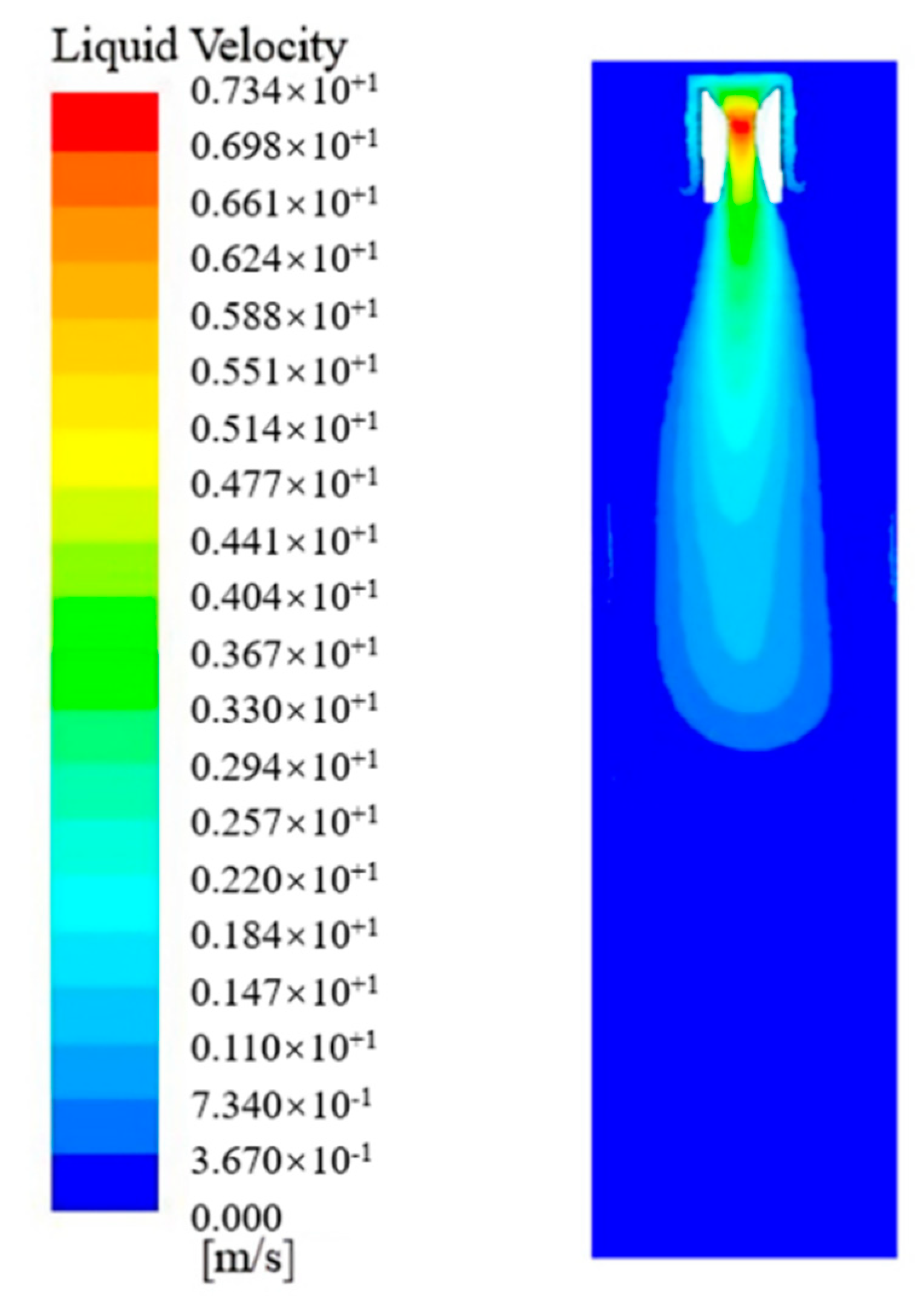
2.1. Data from CFD Simulations

114 CFD simulation datasets extracted from previously published articles [22] were utilized in this study. The structure of the Venturi suction-type gas-liquid distributor [22] is shown in Figure 2, with a throat diameter D, a throat height H, and a throat length L. To accurately show the uniformity of liquid distribution quantitatively, the liquid maldistribution factor $\mathsf{\sigma }$ is defined according to the following Equation [2]:

$$\mathsf{\sigma }=\sqrt{\frac{1}{N\left(N+1\right)}{{\displaystyle \sum }}_{i=1}^N{\left(\frac{u_{L,i}-{\overline{u}}_L}{{\overline{u}}_L}\right)}^2}$$

(1)

where $u_{L,i}$ is the liquid flow rate in zone i, N is the number of zones (11 in this case), and ${\overline{u}}_L$ is the mean flow rate of all zones. As defined, the liquid maldistribution factor varies from 0 (representing the ideal distribution) to 1 (where all liquid flows into a certain region). Thus, a small maldistribution factor value qualifies a better distribution. The liquid flow rate is associated with the sampling plane position and the radial position of the trickle bed. In this paper, we assume that the catalyst bed is located 300 mm below the gas-liquid distributor plane (i.e., the sampling plane). Velocity sampling is performed at the center of the sampling plane, located at 0 mm, and 5 radius positions (30 mm, 50 mm, 70 mm, 90 mm, and 110 mm), for a total of 6 positions. Hence, the radial radius is also used as an input variable of SVR.

In summary, there are four input variables: the throat diameter (D), the throat height (H), the throat length (L), and radial radius (R). The liquid flow rate through zone i ($u_{L,i}$) is used as the output variable, and the maldistribution factor $\mathsf{\sigma }$ as the indirect output variable. The input and output variables of the SVR model and part of the corresponding simulation data from the CFD are summarized in

Table 1. Input and output variables of the support vector regression (SVR) model.

Input Variables				Output Variables
${\mathit{x}}_{\mathbf{1}}$	${\mathit{x}}_{\mathbf{2}}$	${\mathit{x}}_{\mathbf{3}}$	${\mathit{x}}_{\mathbf{4}}$	${\mathit{y}}_{\mathbf{1}}$	$\widehat{\mathit{y}}$
D (mm)	H (mm)	L (mm)	R (mm)	${\mathit{u}}_{\mathit{L}\mathbf{,}\mathit{i}}$	$\mathsf{\sigma }$
40	75	15	90	0.05168	0.307
60	75	15	0	0.78804	0.281
20	75	15	50	0.68672	0.187
50	100	15	70	0.15530	0.276
30	50	0	0	0.89510	0.283
$⋮$
30	25	15	50	0.59876	0.253
30	75	15	0	0.95211	0.239
50	75	15	110	0.05073	0.270
30	50	5	110	0.02788	0.301
30	50	20	30	0.62597	0.295

.

The operating parameters for CFD simulations and the properties of oil are shown in

Table 2. Properties of oil materials and operating parameters used.

Operating Parameters/Physical Parameter	Value
Pressure, MPa	5
Hydrogen−oil ratio, Nm3 · m−3	706
Operating temperature, °C	350
Liquid density, kg · m−3	694
Liquid viscosity, kg · m−1 · s−1	0.00038
Liquid phase velocity, m · s−1	0.23
Gas phase density, kg · m−3	30.6
Gas phase viscosity, kg · m−1 · s−1	0.000015
Vapor velocity, m · s−1	0.24

. The Euler gas-liquid two-phase flow model was used for the simulation, and the Schiller–Naumann drag force model was used between the two phases. The time step was 0.005 s, and the total number of meshes was 173,800.

In the previous work [22] by Zhao, often only one factor was considered for each experiment or calculation, which ignores the interaction among factors. It is essential to consider the correlation between structural parameters of the gas-liquid distributor.

2.2. Support Vector Regression and Particle Swarm Optimization

Support vector regression (SVR) is a machine learning algorithm based on statistical theory, specifically, the principle of structural risk minimization to better solve polynomial regression problems [23,24]. In SVR, the objective function is convex, meaning that the global optimum is always reached. An abstraction of an SVR model with some kernel functions K(x_i, x) is shown in Equation (2).

$$f\left(x\right)={{\displaystyle \sum }}_i^l{\omega }_i\times K\left(x_i,x\right)+b$$

(2)

When solving a nonlinear regression problem, we actually solve for the weights ω_i and the threshold b. Our objective is to use the estimated values of ω_i and b to minimize the regression risk by considering Equations (3) and (4).

$$\min J=\raisebox{1ex}{$1$}\!\left/ \!\raisebox{-1ex}{$2$}\right.{{\displaystyle \Vert }\omega {\displaystyle \Vert }}^2+C{{\displaystyle \sum }}_{i=1}^m\left({\xi }_i^{*}+{\xi }_i\right)$$

(3)

$$s.t.\{\begin{array}{c}{y}_i-\left(\omega ·\varphi \left(x\right)\right)-b\le \epsilon +{\xi }_i\\ \left(\omega ·\varphi \left(x\right)\right)+b-y_i\le \epsilon +{\xi }_i^{*}\\ {\xi }_i,{\xi }_i^{*}\ge 0 \end{array}$$

(4)

where ω is the weight vector, $\raisebox{1ex}{$1$}\!\left/ \!\raisebox{-1ex}{$2$}\right.{\displaystyle \Vert }\omega {{\displaystyle \Vert }}^2$ is the model complexity, and C is the penalty factor, ε is insensitive loss, ${\xi }_i$、${\xi }_i^{*}$ is the relaxation variable.

The Lagrange equation is used to solve this quadratic programming problem, and it is converted into the dual optimization corresponding to Equations (5) and (6).

$$\max J\left(\alpha \right)=\max \{-\frac{1}{2}{{\displaystyle \sum }}_{\begin{array}{c}i=1\\ j=1\end{array}}^m\left({\alpha }_i-{\alpha }_i^{*}\right)·\left({\alpha }_j-{\alpha }_j^{*}\right)K\left(x_i,x_j\right)-\epsilon {{\displaystyle \sum }}_{i=1}^m\left({\alpha }_i+{\alpha }_i^{*}\right)+{{\displaystyle \sum }}_{i=1}^m{y}_i\left({\alpha }_i-{\alpha }_i^{*}\right)\}$$

(5)

$$s.t.\{\begin{array}{c}{\displaystyle {\displaystyle \sum }_{i=1}^m}\left({\alpha }_i-{\alpha }_i^{*}\right)=0\\ 0\le {\alpha }_i\le C \\ 0\le {\alpha }_i^{*}\le C \end{array}$$

(6)

where ${\alpha }_i$, ${\alpha }_i^{*}$, ${\alpha }_j$ and ${\alpha }_j^{*}$ are Lagrangian operators and$K\left(x_i,x_j\right)$ is a kernel function, for which the following holds:

$$f\left(x\right)={{\displaystyle \sum }}_{i=1}^l\left({\alpha }_i-{\alpha }_i^{*}\right)K\left(x_i,x_j\right)+b.$$

(7)

The nonlinear regression function f(x) is obtained through the calculation of the kernel function. The selection of the kernel function affects the non-linear mapping of the samples directly, and so choosing an appropriate kernel function is very important for SVR [25]. The Radial Basis Function (RBF) function [26] is used as the kernel function in this paper because of its excellent generalization and nonlinear regression ability. Its description is showed as below:

$$K\left(x_i,x_j\right)=\exp \left(-\mathrm{g}\Vert x-x_i{\Vert }^2\right)$$

(8)

where g is a kernel function parameter.

In this study, the input and output variables of SVR model is described as Equation (9):

$$u_{L,i}=f\left(D,H,L,R\right).$$

(9)

The prediction performance of SVR is closely related to the RBF kernel parameter g, the penalty factor C, and the insensitive loss ε [27]. In order to obtain a support vector regression machine with better performance, particle swarm optimization (PSO) is adopted for parameter optimization in this paper. Five-fold cross-validation [28] is used to evaluate the fitness of each particle in the PSO algorithm to improve the model prediction performance. It is essential to set a lower limit for the root mean square error (RMSE) in the PSO optimization process to prevent the SVR model from overfitting. When the RMSE is less than the lower limit, the optimization process is ended. The calculation formula of RMSE is as follows:

$$\mathrm{RMSE}=\sqrt{\frac{1}{n}{{\displaystyle \sum }}_{i=1}^n{\left(y_i-f\left(x_i\right)\right)}^2}$$

(10)

where n is the number of samples; $y_i$ is the true value and $f\left(x_i\right)$ is the predicted value of the model. The PSO algorithm aims to minimize the overall error of the model.

After 60 iterations, the RMSE of the training set after 5-fold cross-validation is 1.215 × 10⁻³, and the optimization results of c, g, and ε are 163, 0.737, and 0.241, respectively. The training set and the optimized C, g, and ε values were then applied to the SVR model for training. Then, the test set was input to the trained SVR model to obtain the corresponding predicted value. Finally, the performance of the model was evaluated by comparing the prediction values and the real values.

2.3. Evaluation Index

The validity of the PSO-SVR model was evaluated by comparing the accuracy and rapidity of the algorithm. For comparison purposes, the normalized mean square error (MSE) and the coefficient of determination (R²) were used as performance indicators.

$$MSE=\frac{1}{n}{{\displaystyle \sum }}_{i=1}^n{\left(y_i-f\left(x_i\right)\right)}^2$$

(11)

$${\mathrm{R}}^2=\frac{{{\displaystyle \sum }}_{i=1}^n{\left(f\left(x_i\right)-\overline{y}\right)}^2}{{{\displaystyle \sum }}_{i=1}^n{\left(y_i-\overline{y}\right)}^2}$$

(12)

where n is the number of samples; y_i is the true value; f(x_i) is the value predicted by the model; and $\overline{y}$ is the average of the true values. A smaller MSE is indicative of higher model prediction accuracy. R² ranges from 0 to 1 and is the degree of correlation between the experimental and predictive values. A higher R² value corresponds to better agreement between observed and simulated results. Here, a higher R² value and a lower MSE value indicate a better prediction performance.

3. Optimal Structure Obtained from RSM Based on the PSO-SVR Model

The data obtained using the PSO-SVR hybrid model were applied as the input for the response surface methodology (RSM) to obtain the optimal structural parameters of the distributor.

Response Surface Methodology

RSM is a simple model-based mathematical tool with a low computational burden for predicting and optimizing engineering problems [29]. It mainly uses a reasonable experimental design method and obtains a polynomial equation to describe the behavior of a dataset with the objective of making statistical previsions, while a neural network and PSO cannot be used for such a formulation.

In this article, three structural parameters, namely throat diameter D, throat height H, and throat length L in a Venturi gas-liquid distributor, were selected as influencing factors. The domain of the three structural parameters was determined according to the structure of hydrogenation reactor [22]. The maximum and minimum values of the three factors were input to the Design-Expert design software. 53 structural combinations of the three factors and five levels were obtained by user-defined experimental design. The PSO-SVR model was used as the proxy model to obtain the liquid maldistribution factor $\mathsf{\sigma }$ corresponding to various structural combinations of the Venturi gas-liquid distributor, as shown in

Table 3. Experimental plan designed by response surface methodology (RSM) and corresponding responses.

Sample No.	Throat Diameter, D	Throat Height, H	Throat Length, L	$\mathbf{Response}(\mathbf{Liquid}\mathbf{Maldistribution}\mathbf{Factor},\mathsf{\sigma })$
1	40	100	20	0.3767
2	20	100	10	0.2729
3	40	62.5	15	0.2502
4	60	25	20	0.3629
5	50	43.75	15	0.2499
6	30	81.25	5	0.3113
7	20	62.5	0	0.2621
⋮
49	40	25	0	0.3082
50	60	62.5	10	0.3656
51	50	43.75	10	0.3376
52	30	62.5	15	0.2355
53	20	100	20	0.2663

.

The quartic regression, Equation (13), was applied to find the interaction relationship between the three structural parameters and the liquid maldistribution factor as follows:

$$\begin{array}{cc}\widehat{\mathsf{\sigma }}=+0.34 +& 0.088\times \mathrm{D}+0.069\times \mathrm{H}-0.14\times \mathrm{L}+0.1\times \mathrm{D}\times \mathrm{H}-0.11\times \mathrm{D} \times \mathrm{L}\\ & -0.056\times \mathrm{H} \times \mathrm{L}-0.13\times {\mathrm{L}}^2-0.059\times {\mathrm{D}}^2 \times \mathrm{H}-0.015\times {\mathrm{D}}^2\times \mathrm{L}\\ & -0.037\times \mathrm{D}\times {\mathrm{H}}^2-0.031\times {\mathrm{D}}^3-0.038\times {\mathrm{H}}^3+0.15\times {\mathrm{L}}^3\\ & +0.027\times {\mathrm{D}}^2\times {\mathrm{L}}^2-0.072\times {\mathrm{D}}^3\times \mathrm{H}+0.1\times {\mathrm{D}}^3\times \mathrm{L}\\ & +0.049\times {\mathrm{H}}^3\times \mathrm{L}-0.018\times {\mathrm{D}}^4+0.026\times {\mathrm{H}}^4+0.12\times {\mathrm{L}}^4\end{array}$$

(13)

Normally, the analysis of variance (ANOVA) is considered a very important tool in finding the best fitting mathematical regression model.

Table 4. Analysis of variance (ANOVA) for liquid maldistribution by quartic modeling.

Source	Sum of Squares	df	Mean Square	F Value	p-Value Prob > F
Model	0.17	20	8.482 × 10−3	43.41	<0.0001
D	0.019	1	0.019	98.37	<0.0001
H	0.012	1	0.012	60.36	<0.0001
L	0.049	1	0.049	250.70	<0.0001
D × H	4.524 × 10−3	1	4.524 × 10−3	23.15	<0.0001
D × L	5.073 × 10−3	1	5.073 × 10−3	25.96	<0.0001
H × L	1.341 × 10−3	1	1.341 × 10−3	6.86	0.0133
L2	4.157 × 10−3	1	4.157 × 10−3	21.28	<0.0001
D2 × H	0.014	1	0.014	73.31	<0.0001
D2 × L	9.267 × 10−4	1	9.267 × 10−4	4.74	0.0369
D × H2	5.669 × 10−3	1	5.669 × 10−3	29.01	<0.0001
D3	1.549 × 10-3	1	1.549 × 10−3	7.93	0.0083
H3	2.348 × 10−3	1	2.348 × 10−3	12.01	0.0015
L3	0.035	1	0.035	180.89	<0.0001
D2 × L2	1.281 × 10−3	1	1.281 × 10−3	6.55	0.0154
D3 × H	2.071 × 10−3	1	2.071 × 10−3	10.60	0.0027
D3 × L	4.035 × 10−3	1	4.035 × 10−3	20.65	<0.0001
H3 × L	9.451 × 10−4	1	9.451 × 10−4	4.84	0.0352
D4	1.013 × 10−3	1	1.013 × 10−3	5.19	0.0296

shows a valid model obtained from ANOVA. The p-value of the model obtained in this experiment was far less than 0.05, which indicates that the obtained regression equation is statistically significant.

Table 5. Statistical analysis of regression equation errors.

Statistics Project	Value
Std. Dev.	0.014
Mean	0.33
CV %	4.22
PRESS	0.018
R-Squared	0.9644
Adj R-Squared	0.9422
Pred R-Squared	0.8981
Adeq Precision	27.651

shows the statistical analysis of the regression equation’s error. R² = 0.9644 indicates that there is a statistical goodness of fit between the model and the experimental data. The good agreement between the predicted R² value of 0.8981 and the adjusted R² value of 0.9422 indicates that the model gives a good estimation of response in the studied range. The coefficient of variation (CV) was 4.22%, i.e., less than 10%, which is indicative of the high reliability and accuracy of the regression equation. As a ratio of signal effectiveness, our Adeq Precision of 27.651 was greater than 4, which demonstrates the high rationality of the regression equation.

The 3D response surface plots for the liquid maldistribution factor illustrate the influence of structural parameters and the interactions on the response, as shown in Figure 3. The combined effects of D and H, D and L, H and L on liquid maldistribution factor σ were depicted in Figure 3a–c, respectively. Liquid maldistribution factor σ decreases with the increase of throat length L and the decrease of throat diameter D. The response surface results show that the longer throat length L and the smaller throat diameter D, the better it is to reduce liquid maldistribution σ, while the impact of throat height H is less significant.

The RSM optimization was carried out to minimize the liquid maldistribution factor. The optimal response combination was obtained for a throat diameter D of 20 mm, a throat height H of 84.5 mm, and a throat length L of 16.4 mm, and a liquid maldistribution factor $\mathsf{\sigma }$ of 0.162. For comparison, the optimal structure proposed by Zhao was D = 30 mm, H = 50 mm, L = 15 mm, and $\mathsf{\sigma }$ = 0.184. The optimal estimate of the liquid maldistribution factor in this paper is lower than reported by Zhao et al.

4. Results and Discussion

4.1. Effectiveness Evaluation of the PSO-SVR Model

The validity of the PSO-SVR model as the proxy model was evaluated by comparing the accuracy rapidity of the algorithm.

4.1.1. Comparison and Discussion on the Precision of PSO-SVR Model

Figure 4 shows the prediction results of training and test samples of the PSO-SVR model. The abscissa represents the simulation value of the apparent linear velocity of the liquid obtained using CFD [22], and the ordinate represents the output predicted value of the PSO-SVR model. The samples of the training set and the test set are all concentrated in the diagonal attachment, which indicates that the prediction results are consistent with the experimental data. As shown in Figure 4, the MSE of the PSO-SVR model for the training set was 2.364 × 10⁻⁴ and the coefficient of determination R² was 0.991, which shows a high training accuracy. The normalized MSE of the test set was 5.391 × 10⁻⁴ and the coefficient of determination R² was 0.985, which shows that the prediction result is still good. Therefore, the PSO-SVR model can be used as a proxy model to predict the liquid distribution of the gas-liquid distributor accurately.

4.1.2. Comparison and Discussion on the Rapidity of PSO-SVR Model

The comparison result of the SVR algorithm optimized with the grid search method and the PSO-SVR model is shown in

Table 6. Comparison of evaluation parameters between particle swarm optimization-support vector regression (PSO-SVR) and support vector regression (SVR).

	{C, g, ε}	MSE	R2	CPU Time
PSO-SVR	{C = 163, g = 0.737, ε = 0.241}	5.391 × 10−4	0.985	36.15 s
SVR	{C = 5.6569, g = 1.071, ε = 0.01}	1.314 × 10−3	0.976	1047 s

. Optimizing the SVR parameters using PSO yielded a result of {C = 163, g = 0.737, ε = 0.241}, while optimization using the grid search method resulted in {C = 5.6569, g = 1.071, ε = 0.01}. The MSE of the PSO-SVR model was 5.391 × 10⁻⁴, and R² was 0.985, while the MSE of the SVR model was 1.314 × 10⁻³, and R² was 0.976. The CPU time required by the SVR with the standard grid method and PSO-SVR (t = 1047 s and 36.15 s, respectively). The results show that, as a very effective evolutionary algorithm, the PSO can replace the standard grid search method to find better model parameters and improve the optimization speed and accuracy.

4.2. Verification of the Optimal Structure

To verify the credibility of the optimal structure of the gas-liquid distributor proposed in this paper, CFD simulations were conducted using ANSYS FLUENT V15.00 and run on a high-performance computing (HPC) system. The computations were carried out using an Intel Xeon (R) Gold 5118 processor with 24 CPU cores. As far as the boundary conditions are concerned, velocity-inlet conditions were used at the domain inlet and a pressure outlet condition was specified at the domain exit. The physical properties and initial speed were set according to the properties of oil materials and operating parameters in Table 2. The input speed of the single distributor was 0.02987 m/s, and the cylindrical wall surface was set as an adiabatic, non-slip wall surface. The standard k-ε model was selected as the turbulence model, using the SIMPLE-algorithm for the pressure-velocity coupling. The 3D non-steady state was taken as the initial condition for calculation. With a time step of 0.005 s, converge was achieved at 150 s for residual curve values of all the equations constantly stable below 0.001.

The velocity distribution contour of the gas-liquid distributor converging to steady state is shown in Figure 5. The velocity distribution of the oil materials at 300 mm below the gas-liquid distributor tray is obtained as 1.4633, 1.3517, 1.0972, 0.7715, 0.4911, 0.2405 at the sampling position mentioned in Section 2.1. Maldistribution factor $\mathsf{\sigma }$ was calculated as 0.159 according to Equation (1), which is in good agreement with the value of 0.162 obtained using RSM.

The distribution performance of the distributor with the optimal structure is analyzed according to the liquid velocity distribution contour shown in Figure 5. After falling into the distribution tray, the materials continue to pile up, and then enter the dispenser under the suction of the slit. In this process, the gas and liquid phases are violently mixed. While the continuous liquid phase is broken by the gas phase, it flows upward along the channel, and the materials in different directions crash above the downcomer and flow downward. Due to the improved Venturi structure existing in the gas-liquid distributor, the flow area at the throat position decreases sharply, with the velocity of oil materials reaching a maximum speed of 7.34 m/s. The accumulation of materials in the position of the throat causes a large pressure above the throat, and a high-pressure difference is forming under the throat. The material fills the outlet section quickly when it flows out through the throat under the effect of the pressure difference. The inclined outlet section in the Venturi structure produces a larger diffusion angle when the material flows out of the distributor, thus a larger radial distribution of the material on the catalyst bed is achieved.

5. Conclusions

In this study, we investigate the utility of using the PSO algorithm for optimizing the parameters of SVR in order to obtain an effective hybrid model (PSO-SVR) for application in modeling liquid maldistribution of the gas-liquid distributor in TBRs. The hybrid PSO-SVR model was based on limited CFD simulation data to replace the time-consuming CFD simulation for different cases, with a very low time cost for accurately predicting the results of the liquid distribution. RSM was used to predict the optimal structure of the gas-liquid distributor in TBRs based on the PSO-SVR model. To ensure the accurate values of the best structural parameters obtained using RSM, another simulation of these structural was performed using CFD to determine the liquid maldistribution. The CFD simulation results reaffirmed the accuracy of the optimal structure proposed in this paper.

The model development, experiment design, and CFD validation are coupled with the following concluding remarks:

(1)

SVR was used with limited CFD simulation data to overcome the high computational load issue of CFD and achieve an accurate mathematical model.

(2)

The PSO algorithm was employed to determine an optimal set of parameters of the SVR model and speed up modeling.

(3)

The optimal structure of gas-liquid distributor was obtained from the combination of PSO-SVR and RSM.

(4)

RSM was applied to clarify the influence of structural parameters of the gas-liquid distributor on the liquid maldistribution.

(5)

A closed-loop optimized system was designed beginning from collecting CFD data, modeling with PSO-SVR, optimizing by RSM, and ending with CFD validation.

The closed-loop optimized system proposed in this manuscript could also be applied to the modeling and optimization of chemical process, as well as related chemical equipment structure.

References

1. Atta, A.; Roy, S.; Nigam, K.D.P. Investigation of liquid maldistribution in trickle-bed reactors using porous media concept in CFD. Chem. Eng. Sci. 2007, 62, 7033–7044. [Google Scholar] [CrossRef]
2. Marcandelli, C.; Lamine, A.S.; Bernard, J.R.; Wild, G. Liquid Distribution in Trickle-Bed Reactor. Oil Gas. Sci. Technol. 2000, 55, 407–415. [Google Scholar] [CrossRef] [Green Version]
3. Kundu, A.; Saroha, A.K.; Nigam, K.D.P. Liquid distribution studies in trickle-bed reactors. Chem. Eng. Sci. 2001, 56, 5963–5967. [Google Scholar] [CrossRef]
4. Li, M.; Iida, N.; Yasuda, K.; Bando, Y.; Nakamura, M. Effect of orientation of packing structure on liquid flow distribution in trickle bed. J. Chem. Eng. Jpn. 2000, 33, 811–814. [Google Scholar] [CrossRef]
5. Zalucky, J.; Wagner, M.; Schubert, M.; Lange, R.; Hampel, U. Hydrodynamics of descending gas-liquid flows in solid foams: Liquid holdup, multiphase pressure drop and radial dispersion. Chem. Eng. Sci. 2017, 168, 480–494. [Google Scholar] [CrossRef]
6. Roy, S.; Kamalanathan, P.; Al-Dahhan, M. Integration of phase distribution from gamma-ray tomography technique with monolith reactor scale modeling. Chem. Eng. Sci. 2019, 200, 27–37. [Google Scholar] [CrossRef]
7. Wu, H.; Buschle, B.; Yang, Y.; Tan, C.; Dong, F.; Jia, J.; Lucquiaud, M. Liquid distribution and hold-up measurement in counter current flow packed column by electrical capacitance tomography. Chem. Eng. J. 2018, 353, 519–532. [Google Scholar] [CrossRef]
8. Singh, B.K.; Jain, E.; Buwa, V.V. Feasibility of Electrical Resistance Tomography for measurements of liquid holdup distribution in a trickle bed reactor. Chem. Eng. J. 2019, 358, 564–579. [Google Scholar] [CrossRef]
9. Lovreglio, P.; Das, S.; Buist, K.A.; Peters, E.A.J.F.; Pel, L.; Kuipers, J.A.M. Experimental and numerical investigation of structure and hydrodynamics in packed beds of spherical particles. AIChE J. 2018, 64, 1896–1907. [Google Scholar] [CrossRef]
10. Uribe, S.; Cordero, M.E.; Reyes, E.P.; Regalado-Méndez, A.; Zárate, L.G. Multiscale CFD modelling and analysis of TBR behavior for an HDS process: Deviations from ideal behaviors. Fuel 2019, 239, 1162–1172. [Google Scholar] [CrossRef]
11. He, G.; Mo, H.; Zhang, R.; Jin, H.; Du, W. Study of the effects of walls on vortex formation and liquid maldistribution with two-phase flow around a spherical particle via numerical simulation. Powder Technol. 2019, 354, 125–135. [Google Scholar] [CrossRef]
12. Shah, M.T.; Utikar, R.P.; Pareek, V.K. Effect of column inclination and oscillation on liquid spreading in a trickle bed. Chem. Eng. Res. Des. 2019, 152, 165–179. [Google Scholar] [CrossRef]
13. Klenov, O.P.; Noskov, A.S. Influence of input conditions on the flow distribution in trickle bed reactors. Chem. Eng. J. 2020, 382. [Google Scholar] [CrossRef]
14. Dhanraj, D.I.A.; Buwa, V.V. Effect of capillary pressure force on local liquid distribution in a trickle bed. Chem. Eng. Sci. 2018, 191, 115–133. [Google Scholar] [CrossRef]
15. Mehmani, A.; Chowdhury, S.; Meinrenken, C.; Messac, A. Concurrent surrogate model selection (COSMOS): Optimizing model type, kernel function, and hyper-parameters. Struct. Multidiscip. Optim. 2018, 57, 1093–1114. [Google Scholar] [CrossRef]
16. Cheng, K.; Lu, Z. Adaptive sparse polynomial chaos expansions for global sensitivity analysis based on support vector regression. Comput. Struct. 2018, 194, 86–96. [Google Scholar] [CrossRef]
17. Xiang, H.; Li, Y.; Liao, H.; Li, C. An adaptive surrogate model based on support vector regression and its application to the optimization of railway wind barriers. Struct. Multidiscip. Optim. 2017, 55, 701–713. [Google Scholar] [CrossRef]
18. Zhang, W.; Zhang, L.; Yang, J.; Hao, X.; Guan, G.; Gao, Z. An experimental modeling of cyclone separator efficiency with PCA-PSO-SVR algorithm. Powder Technol. 2019, 347, 114–124. [Google Scholar] [CrossRef]
19. Bansal, S.; Roy, S.; Larachi, F. Support vector regression models for trickle bed reactors. Chem. Eng. J. 2012, 207–208, 822–831. [Google Scholar] [CrossRef]
20. Jalalifar, S.; Masoudi, M.; Abbassi, R.; Garaniya, V.; Ghiji, M.; Salehi, F. A hybrid SVR-PSO model to predict a CFD-based optimised bubbling fluidised bed pyrolysis reactor. Energy 2020, 191. [Google Scholar] [CrossRef]
21. Zaidi, S. Development of support vector regression (SVR)-based model for prediction of circulation rate in a vertical tube thermosiphon reboiler. Chem. Eng. Sci. 2012, 69, 514–521. [Google Scholar] [CrossRef]
22. Zhao, F. Study on Fluid Flow Characteristics and Lumped Reaction Kinetics in Hydrogenation Reactor; China University of Petroleum: Beijing, China, 2016. [Google Scholar]
23. Tabari, M.M.R.; Sanayei, H.R.Z. Prediction of the intermediate block displacement of the dam crest using artificial neural network and support vector regression models. Soft Comput. 2019, 23, 9629–9645. [Google Scholar] [CrossRef]
24. Yang, H.; Nikafshan Rad, H.; Hasanipanah, M.; Bakhshandeh Amnieh, H.; Nekouie, A. Prediction of Vibration Velocity Generated in Mine Blasting Using Support Vector Regression Improved by Optimization Algorithms. Nat. Resour. Res. 2020, 29, 807–830. [Google Scholar] [CrossRef]
25. Hasanipanah, M.; Shahnazar, A.; Bakhshandeh Amnieh, H.; Jahed Armaghani, D. Prediction of air-overpressure caused by mine blasting using a new hybrid PSO–SVR model. Eng. Comput. 2017, 33, 23–31. [Google Scholar] [CrossRef]
26. Akinpelu, A.A.; Ali, M.E.; Owolabi, T.O.; Johan, M.R.; Saidur, R.; Olatunji, S.O.; Chowdbury, Z. A support vector regression model for the prediction of total polyaromatic hydrocarbons in soil: An artificial intelligent system for mapping environmental pollution. Neural Comput. Appl. 2020, 3. [Google Scholar] [CrossRef]
27. Zuo, Q.; Zhu, X.; Liu, Z.; Zhang, J.; Wu, G.; Li, Y. Prediction of the performance and emissions of a spark ignition engine fueled with butanol-gasoline blends based on support vector regression. Environ. Prog. Sustain. Energy 2019, 38, 1–9. [Google Scholar] [CrossRef]
28. Chen, H.; Liu, C.; Xu, X.; Zhang, L. A new model for predicting sulfur solubility in sour gases based on hybrid intelligent algorithm. Fuel 2020, 262, 116550. [Google Scholar] [CrossRef]
29. Keshtegar, B.; Heddam, S.; Sebbar, A.; Zhu, S.P.; Trung, N.T. SVR-RSM: A hybrid heuristic method for modeling monthly pan evaporation. Environ. Sci. Pollut. Res. 2019, 26, 35807–35826. [Google Scholar] [CrossRef]
Figure 1. The flow chart for obtaining an optimized solution of the gas-liquid distributor in trickle-bed reactors (TBRs).
Processes 08 01332 g001
Figure 2. Structure of Venturi suction-type gas-liquid distributor.
Processes 08 01332 g002
Figure 3. 3D plot of response surface for liquid maldistribution factor σ. (a) Throat diameter D and throat height H combination; (b) throat diameter D and throat length L combination; (c) throat height H and throat length L combination.
Processes 08 01332 g003
Figure 4. The prediction results of training and test samples.
Processes 08 01332 g004
Figure 5. Velocity contour of Venturi distributor at central surface.
Processes 08 01332 g005