CFD Hydrodynamics Investigations for Optimum Biomass Gasifier Design

Abstract

Biomass gasification is nowadays considered a viable option for clean energy production. Furthermore, still more efforts need to be spent to make this technology fully available at commercial scale. Drawbacks that greatly limit the full-time plant availability—and so its economically feasibility—mainly concerns syngas purification by contaminants such as tars. Different technological approaches were investigated over last two decades with the aim to increase both the plant availability and the overall efficiency by keeping, at the same time, CAPEX and OPEX low. Among technologies, fluidized beds are surely the most promising architectures for power production at thermal scale above 1 MW_th. Gasifier can be surely considered the key component of the whole power plant and its proper design, the main engineering effort. This process involves different engineering aspects: thermo-structural, heat, and mass transfer, and chemical and fluid-dynamic concerns being the most important. In this study, with the aim to reach an optimal reaction chamber design, the hydrodynamics of a bubbling fluidized bed reactor was investigated by using a CFD approach. A Eulerian–Eulerian multiphase model, supported by experimental data, was implemented to describe the interactions between the solid and fluid phases inside the reactor while a discrete dense phase model (DDPM) model was considered to investigate momentum exchange among continuous phases and solid particles simulating char. Different process parameters, such as the bed recirculation rate and the particles circulation time inside the bed, were at least analyzed to characterize the hydrodynamics of the reactor. Results indicate that the recirculation time of bed material is in the order of 6–7 s at bench scale and, respectively, of 15–20 s at full scale. Information about solid particles inside the bed that should be used to avoid elutriation and agglomeration phenomenon, suggest that the dimension of the mother fuel particles should not exceed the value of 5–10 mm.

1. Introduction

Amongst all energy sources for power generation, renewables had in the last decade the highest rate of growth. IEA (International Energy Agency) projections in its SDS (Sustainable Development Scenario), project bioenergy share by 2030 from by the actual 590 TWh (2019) to about 1170 TWh (2030), with an annual increase of 6% (electricity generation from bioenergy) [1]. Moreover, it is expected that several policies and market initiatives will encourage this trend. In some countries such as China, where use biomass fueled power plant is actually promoted by feed-in tariff, development of biomass fueled power plant, is expected to great extent. The overall goal is to improve air quality to meet environmental policies supporting the phase out of coal-fired boilers and the uncontrolled burning of agricultural residues in the field it a self. As China other countries, such as Brazil and India are implementing similar policies to encourage the development of bioenergy as a way to support in a sustainably manner the to meet their ever increasing energy demand. In this context energy production by biomass will surely have a key role. Furthermore, it must be considered that biomass is the only renewable source of carbon that can be converted conveniently to solid, liquid, and gaseous products by mean different process [2]. Amongst different technologies available today for biomass conversion, gasification is considered to have the greatest potential due its higher thermochemical conversion efficiency [3]. Gasification is a thermochemical process that occurs inside reactors known as gasifiers where solid feedstocks are converted in gaseous form at high temperature (typically in the range of 700–900 °C). Via gasification, a fraction of the initial chemical energy is stored into the producer gas: in such processes about 80% (cold efficiency) of the original energy is converted. Gaseous form is most suitable for different kinds of application for power production such as internal combustion engines, fuel cells, and gas turbines. Furthermore, syngas can be converted to fuel catalytically via FT (Fischer Tropsch) synthesis [4]. Depending on the end-use of syngas on power scale plant, though different gasifier architectures can be considered but mainly two main groups, namely, fixed beds and fluidized beds, are available. Fixed beds for power production (downdraft and updraft) are more suitable for small scale application (30–250 kW_e). Most widely used plant architecture is that where downdraft gasifier is coupled to an internal combustion engine. A comprehensive review of technologies available at small scale is provided by [5]. Fluidized beds instead are well applicable at medium–large scale (5–40 MW_e) where plant installation complexities are overcome by the highest added value of the final product (i.e., hydrogen production and chemicals) and by the large power throughput of the plant. From a general point of view fluidized bed reactors overcame some limitations imposed by fixed beds such as the non-uniform distribution of heat and mass transfer inside the reaction chamber and scaling-up related issues. Today fluidized bed reactors are widely used both for industrial purposes and for gas–solid reactions such as biomass gasification. This is mainly due to the relative low temperature achievable inside the bed (800–1000 °C), adequate for lignocellulosic biomass gasification, although low when compared to that required by other solid combustibles, such as coal, where this results in a low carbon conversion efficiency [6]. Surely fluidized bed is a mature technology to generate power and heat, but its application to biomass still imposes some operational problems. Amongst these, agglomeration of the bed material is the major concern especially when lignocellulosic biomass containing potassium, sodium, and alkali earth metal along with chlorine and sulfur are used. The main elements in biomass that create eutectic formations are potassium and sodium in the form of ${\mathrm{K}}_2\mathrm{O}$ and $\mathrm{N}{\mathrm{a}}_2\mathrm{O}$ (potassium is more damaging than sodium) [6]. Different kinds of fluidized bed reactors available, commercially independent of their design, can be operated in three different flow regimes: bubbling, turbulent, or fast fluidization [7]. Bubbling fluidized bed is surely the simplest and cost-affordable concept for biomass gasification at medium scale (1–10 MW_e). They are greatly flexible to a wide range of biomass with various particle sizes. Continuous mixing between inert bed material and solid combustible inside the reaction chamber, promotes a uniform distribution of the temperature along the reaction zone. This reduce hot spot and agglomeration of ashes by formation of low melting eutectic mixture. Furthermore, a uniform producer gas with medium-low tar content (in the order of $~ 10 \mathrm{to} 15 \mathrm{g}/\mathrm{N}{\mathrm{m}}^3$, [8]) and higher carbon conversion is achievable. In circulating fluidized beds, high superficial gas velocity promotes a turbulent flow regime where solid particles (both inert bed material and residual char) are entrained resulting in their circulation between different regions of the reactor. Details about such technologies are provided by [8,9,10,11,12]. Circulating fluidized beds are well suitable for large scale power plant (above 10 MW_th) where large dimensional development of the equipment is well justified.

Common issue of both fixed and fluidized bed reactors is the large quantities of tar in the producer gas that compromises the plant availability. With the aim to increase both the plant availability and the overall efficiency while not compromising with CAPEX and OPEX low, several approaches for tar abatement are today under investigation [3,13]. Amongst these, primary methods that act directly on the formation of tar inside gasifier, can be considered to a viable option. Nevertheless, it must be stated that these methods are not yet well understood and their application at commercial scale is actually limited [3,14,15].

Other than the selection of the right operational conditions and the injection of additives (to prevent also the formation of ashes agglomerates) or catalysts during gasification, the approach used in the gasifier design plays a key role in tar formation mechanisms. In the last two decades efforts have been made to investigate the hydrodynamic of fluidized bed reactors, both experimentally and numerically. The main aim is to well understand phenomenon involved during gas–solid interactions as well as to know how these can influence the reactor behavior. It was because of the complexities involved in the process of biomass gasification (fluid dynamic concerns, heat and mass transfer, kinetic of reactions, and so on) that the gasifier design was mainly based on empirical correlations from experimental derivation on bench scale reactors or pilot plant. Furthermore, such empirical formulas had limited applications under certain conditions [16]. Recent developments in numerical techniques and the availability of computational infrastructures, make the application of CFD affordable to investigate design of fluidized bed reactors and their evaluation. In this field two types of methods can mainly be applied: the Eulerian–Eulerian (E-E) approach and the Eulerian–Lagrange (E-L) approach [17]. The E-E approach considers both fluid and particles in the continuous interpenetrating phases. In such a manner granular solid phase is treated as a pseudo-fluid. The E-L approach still considers fluid phase (i.e., gas phase) as continuous but the granular one, is treated by tracking a large number of particles through the computational domain. The E-E approach is less computational expensive compared to E-L approach and is surely the most widely applied in the study of the hydrodynamic of fluidized beds. In the following text, a brief and not exhaustive summary of some contributions in the field is selected with reference to that considered in this study. Kuramoto et al. (1985) [18], developed a new system for circulating fluidized bed within a single vessel where two distinct sections of the reactor were separated by a vertical plate. The two regions were fluidized by a different flow rate so that a circulation of bed material between them was observed. Furthermore, the authors, experimentally investigated the behavior of the system under different operational conditions demonstrating that the proposed configuration potentially had the same advantages of conventional dual-bed system, and that it can be applied to biomass gasification. Kuramoto et al. (1986) [19], experimentally studied the circulation of dense fluidized particles in a two-dimensional bed which was divided in two portions by a vertical plate with an opening. The tests demonstrated how the circulation rate of solid through the opening was controlled by the superficial gas velocity of the up-flowing chamber and by the ratio between the opening area and the cross-sectional area of the down-flowing chamber. Empirical correlations that coupled opening ratio and pressure drop across the opening were also developed. Di Felice et al. (1991) [20], experimentally evaluated the validity of scaling relationships between a pair of dynamically similar gas fluidized beds confirming their application. The study was extended to a wide range of particles: from fine (Geldart group A) to large particles (Geldart group D). The authors highlighted as scaling relationships fail to explain observed slugging regime characteristics. Nieuwland et al. (1994) [21], developed a one-dimensional model for the riser section of a circulating fluidized bed, which describes the steady-state hydrodynamic inside the chamber. Gas and solid phases were considered as two continuous media fully penetrating each other. Zimmermann et al. (2005) [22], investigated the hydrodynamics and kinetics of gas–solid fluidized bed highlighting how the use of both Gidaspow and Syamlal O’Brien drag law overestimate bed expansion in comparison to experimental data. Moreover, they evaluated as the modified Syamlal O’Brien drag law based on the minimum fluidization conditions well predict both the expected bubbling fluidization behavior and bed expansion if compared to experimental evidences. Foscolo et al. (2007) [23], experimentally investigated the behavior of cold model reactor to confirm the feasibility of the pilot scale reactor configuration consisting of two interconnected bubbling fluidized beds. The configuration studied by Foscolo is the landmark of our reactor development. Actually, 1 MW_th biomass gasification pilot plant as result of this study, is working, for research purposes, at the ENEA (Italian National Agency for New Technologies, Energy and Sustainable Economic Development) research center Trisaia at Rotondella. Papadikis et al. (2008–2010) [24,25,26], studied the momentum transport on solid particles, modelling solid fuel, inside bubbling fluidized bed of sand, as continuous. E-E two phases model was implemented to describe the behavior of bubbling bed. Furthermore, kinetic model was implemented to describe gasification reactions inside the reactor. Deza et al. (2009) [27], used a multifluid E-E model to represent the gas and solid phases as continuous. Simulations were carried out to investigate about the behavior of a cold-flow glass bead fluidized bed using as comparison two different drag laws. Numerical data were compared with experimental ones by X-ray flow visualization computed tomography highlighting as Gidaspow model can be used to describe the hydrodynamic of a biomass fluidized bed. Armstrong et al. (2010) [28], used the E-E two-fluid model (TFM) which assumes the gas–solid phases as continuous and fully interpenetrating to evaluate the hydrodynamic behavior of CFB riser during transition from bubbling to circulating fluidized bed. 2D and 3D model were both considered with the implementation of modified drag laws (EMMS). In its study also bubbles diameter was evaluated and compared with the Davinson’s model. All evaluations were reported to be in good agreement with experimental data. Gerber et al. (2010) [29], used an E-E multiphase approach for modeling unsteady wood gasification in fluidized bed reactor. Three interpenetrating continuous phases were used to describe the behavior of dispersed phases inside the reactor: one representing wood and two char with different particles diameter. No inert material was considered inside the bed. 2D simulations that also implemented wood pyrolysis, char gasification, and homogeneous gas phase reactions were carried out by using MFIX code by NETL (National Energy Technology Laboratory). Liu et al. (2013) [30], used a comprehensive 3D model by using E-E approach to simulate biomass gasification in a CFB reactor. Turbulent $k-\epsilon$ model was coupled with the kinetic theory of granular flow to simulate the hydrodynamic of the gas–solid system. Kinetics of homogeneous and heterogeneous reactions were also implemented in the whole model to evaluate the effects of same operation parameters on the performances of the CFB reactor. Bidwe et al. (2014) [22], experimentally investigated cold model of dual fluidized bed system (BFB gasifier and CFB regenerator) for solid fuels gasification by using Glicksman’s simplified scaling ratios. They showed as parameters under investigation can be useful applied (with respect to scaling laws) in the design of the pilot plant. Canneto et al. (2015) [31], numerically studied bubbles formation and their paths to investigate the behavior of the ENEA’s Internally Circulating Bubbling Fluidized Bed (ICBFB) under different fluidization conditions. CFD model by using E-E approach was developed and experimental data from cold model were compared to theoretical ones to study the fluidization quality and to estimate the circulation of solid particles inside the bed. Pecate et al. (2019) [27], experimentally investigate the hydrodynamic of fast internally circulating fluidized bed (FICFB) used for biomass gasification. In its study the influence of bed temperature (between 20 and 950 °C) and the fluidizing agent (air or steam) on the hydrodynamic of a dense fluidized bed of olivine was analyzed. Numerical correlations were used to fit experimental data.

Most of the numerical studies analyzed in the literature are referred to the simple cylindrical geometry of the reactor at bench scale, and many of these are focused only on the evaluation of the main phenomenon involved in the fluidizing process. This work proposes the use of CFD techniques as a new approach to the real rector design by using information achievable by the scaled cold model reactor. In this study the hydrodynamic of the new concept of the ENEA’s ICBFB (Internally Circulating Bubbling Fluidized Bed), as revision of the 1 MW_th pilot plant [32,33], is under investigation. This configuration merges both advantages of bubbling and internally circulating fluidized beds by keeping all reaction zones in only one vessel. A CFD E-E based model, referred to the real geometry of the scaled cold reactor, was implemented to investigate the behavior of the bed. To describe solid–fluid interactions a modified Syamlal O’Brien drag law is considered while DDPM (discrete dense phase model) was used to discretize solid particles modelling char to evaluate both the interactions with solid and fluid phases.

2. Materials and Methods

This work deals about the hydrodynamic optimization of the new configuration of the ENEA’s ICBFB pilot scale reactor, Figure 1. Within only one vessel, two bubbling fluidized beds of different cross-sectional area are delimitated by a vertical plate at the lower edge of which an interconnection opening between them (fluidized beds) is realized. Different flow rate of fluidizing agents (air) are introduced in the two chambers so that different regimes of fluidization are induced. These conditions create, inside the reactor, two areas at different bed density, which promote the circulation of the inert bed material through the opening from the denser chamber (down-flowing bed, DFB) to the lesser one (up-flowing bed, UFB). By varying the difference between the two superficial velocity inside the two reaction chambers, a different circulation rate of bed material is induced.

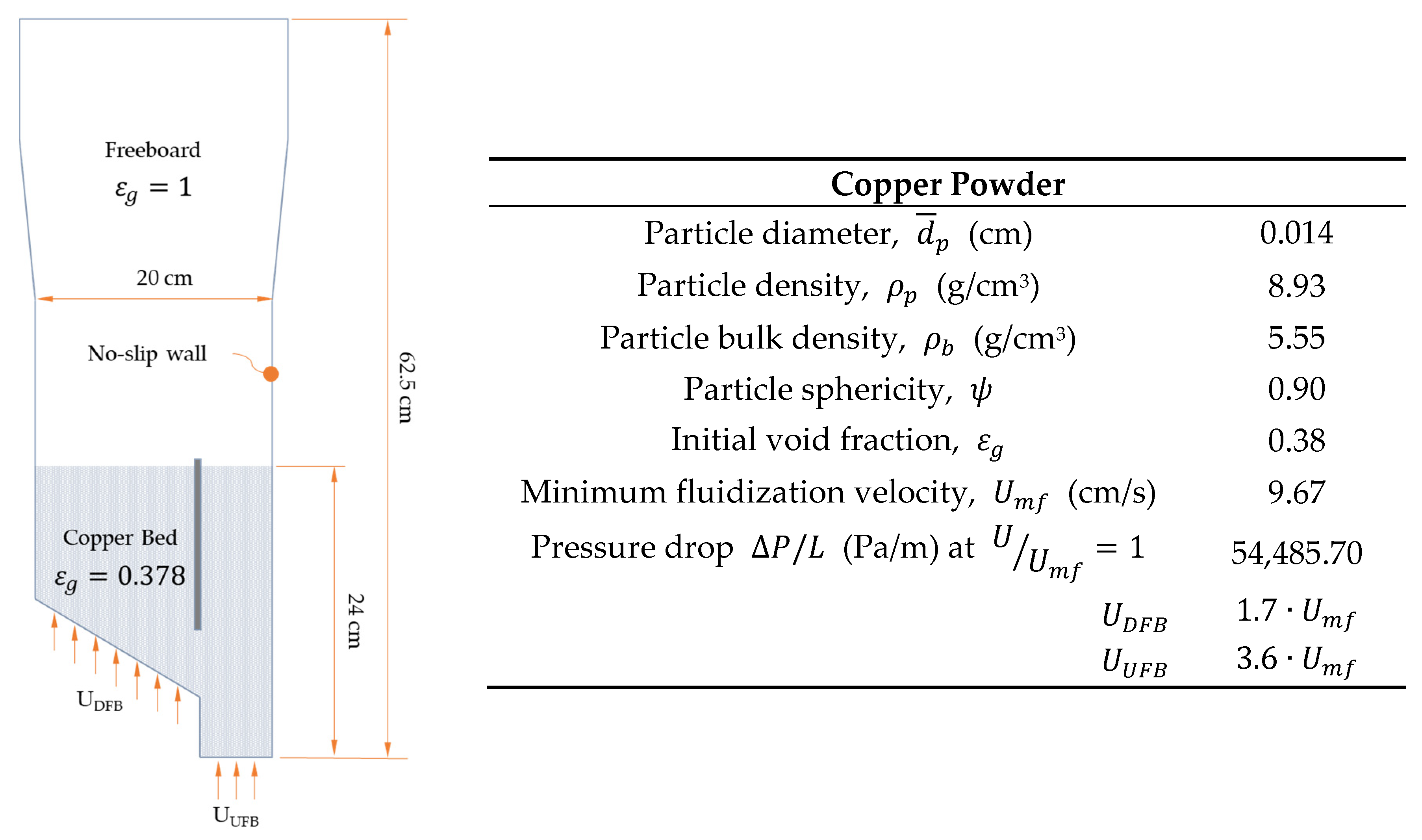
2.1. Cold Model Definition

Numerical investigations were carried out on bench scale cold model reactor in fluid dynamic similar to the real ICBFB pilot plant. For this purpose, scale transposition laws were assumed to be in agreement with some dimensionless parameters (nine dimensional groups) as proposed by Glicksman [34]. In such a manner phenomenon involved and the hydrodynamic behavior observed on bench scaled cold model can directly be transposed to real reactor. Different applications of this criterion as carried out by Kolar and Leckner [35], where a 12 MW_th CFB scale transportation is involved, demonstrate how it is very difficult to meet at the same time, all nine dimensionless groups. In this study, the methodology proposed by Foscolo et al. [23], where only four of these parameters must be satisfied, was considered:

$$\mathrm{Archimedes} \mathrm{number}: Ar=\frac{d_p{}^3·{\rho }_g·\left({\rho }_p-{\rho }_g\right)·g}{{\mu }^2}$$

(1)

$$\mathrm{Density} \mathrm{number}: De=\frac{\rho }{{\rho }_p}$$

(2)

$$\mathrm{Flow} \mathrm{number}: Fl=\frac{U_0}{U_{mf}}$$

(3)

$$\mathrm{Length} \mathrm{number}: Le=\frac{L}{d_p}$$

(4)

with respect to bench scale tests, with known fluidizing flow (i.e., air), well defined temperature, pressure (i.e., reference conditions), and geometry of the real reactor, thus satisfying the above written dimensionless parameters, the geometry of the cold model is fully determined, as well. In addition to such parameters, also the Reynolds and Froude numbers (even if their combination defines the Archimedes number) were verified as, additional conditions:

$$\mathrm{Reynolds} \mathrm{number}: Re=\frac{{\rho }_g·U_o·d_p}{\mu }$$

(5)

$$\mathrm{Froude} \mathrm{number}: Fr=\frac{U_o}{\sqrt{g·d_p}}$$

(6)

Main results of the scaling procedure for the cold model definition are summarized in

Table 1. Cold model definition.

Parameters	Gasifier Reactor 1	Cold Model 2
Fluidizing flow density, ${\rho }_g$ (kg/m3)	0.33	0.99
Fluidizing flow viscosity, $\mu$ (Pa s)	4.38 × 10−5	1.89 × 10−5
Particle density, ${\rho }_p$ (kg/m3)	2965	8930
Archimedes number, $Ar$	6.22 × 102
Reynolds number, $Re$	6.24 × 10−1
Froude number, $Fr$	2.38 × 10−4
Density number, $De$	1.11 × 10−4
Particle diameter, $d_p$ (mm)	0.50	0.14
Minimum fluidization velocity, Umf (cm/s)	16.64	8.71
Length scale ratio, $Le-d_{p GR}/d_{p CM}$	3.65
Gas flow velocity ratio, $Fl$-($U_{GR}/U_{CM}$)	1.91
Gas flow rate ratio, ($Q_{GR}/Q_{CM}$)	25.45
Time ratio, ($t_{GR}/t_{CM}$)	1.91

¹ Gasifier is operated at 800 °C and 1 atm by using air as fluidizing flow. ² Cold Model is operated at 25 °C and 1 bar by using a mixture of air and helium at 3% wt. as fluidizing flow.

. As shown, bed material with particle density of the order of ${\rho }_p\cong 8900 \mathrm{kg}/{\mathrm{m}}^3$ and with particle diameter of about $d_p\cong 0.14 \mathrm{mm}$ must be chosen to meet all scaling parameters.

In addition, the satisfaction of the density number criterion imposes to use as fluidizing flow a medium with density of ${\rho }_g\cong 0.99 \mathrm{kg}/{\mathrm{m}}^3$ at 25 °C. All conditions were satisfied by considering copper powder (${\rho }_p=8930 \mathrm{kg}/{\mathrm{m}}^3$, $d_{p mean}=0.137 \mathrm{mm}$) as bed material and a mixture of air and helium at 3% wt. at 25 °C as fluidizing flow. In conclusion, bench scale reactor, operated in cold flow conditions (25 °C, 1 bar), must be in length scale ratio with the real gasifier of 3.65 (scale 1:3.65) and should use copper powder as bed material and a mixture of air and helium as fluidizing flow.

2.2. Mathematical Model

Eulerian–Eulerian multiphase approach was considered to describe gaseous flow (fluidizing flow as primary phase) and granular solid material (bed material as secondary phase) behavior. As defined earlier in the introduction, all interacting phase are considered, by E-E approach, i.e., as continuous and interpenetrating. The volume fraction occupied by each one phase cannot be occupied by another one:

$${\displaystyle \sum }_{q=1}^n{\epsilon }_q=1$$

(7)

where $n$ is the number of interacting phases, ${\epsilon }_q$ the volume fraction of phase $q$. In addition, each phase must satisfy conservation equations: both continuity and momentum. The first of these, for a generic phase $q$, is expressed by

$$\frac{\partial }{\partial t}\left({\epsilon }_q·{\rho }_q\right)+\nabla ·\left({\epsilon }_q·{\rho }_q·{\overrightarrow{v}}_q\right)={\displaystyle \sum }_{p=1}^n\left(\dot{m_{pq}}-\dot{m_{qp}}\right)+S_q$$

(8)

where $\overrightarrow{v_q}$ is the velocity vector, $\dot{m_{ij}}$ the mass transfer rate between phases $i$ and $j$, $S_q$ the source term for phase $q$ (generally equal to zero). If close system, with no mass transfer between phases is considered, the previous equation is simplified as

$$\frac{\partial }{\partial t}\left({\epsilon }_q·{\rho }_q\right)+\nabla ·\left({\epsilon }_q·{\rho }_q·{\overrightarrow{v}}_q\right)=0$$

(9)

Under the same assumptions and additionally when volume, lift and virtual mass induced forces are negligible, the momentum conservation can be expressed, for gas phase, by

$$\frac{\partial }{\partial t}\left({\epsilon }_g·{\rho }_g·{\overrightarrow{v}}_g\right)+\nabla ·\left({\epsilon }_g·{\rho }_g·{\overrightarrow{v}}_g·{\overrightarrow{v}}_g\right)=-{\epsilon }_g\nabla p+\nabla ·{\stackrel{=}{\tau }}_g+{\epsilon }_g·{\rho }_g·\overrightarrow{g}+{\displaystyle \sum }_{s=1}^m{\overrightarrow{R}}_{sg}$$

(10)

where $m$ is the number of solid phases that interact with the gaseous one. The first term at left-hand side accounts for unsteady acceleration terms while the second one for the acceleration related to convective flow. At right-hand side, the term ${\epsilon }_g\nabla p$ accounts for pressure variation, while $\nabla ·{\stackrel{=}{\tau }}_g$ represents viscous forces. In this latter, the stress tensor is given by

$${\stackrel{=}{\tau }}_g={\epsilon }_g·{\mathsf{\mu }}_g·\left(\nabla ·{\overrightarrow{v}}_g+\nabla ·{\overrightarrow{v}}_g{}^T\right)+{\epsilon }_g·\left({\lambda }_g-\raisebox{1ex}{$2$}\!\left/ \!\raisebox{-1ex}{$3$}\right.{\mathsf{\mu }}_g\right)·\nabla ·{\overrightarrow{v}}_g·\stackrel{=}{I}$$

(11)

where ${\mathsf{\mu }}_g$ and ${\lambda }_g$ are respectively the cinematic and bulk viscosity of gas flow and $\stackrel{=}{I}$ the identity tensor. The term ${\displaystyle \sum }_{s=1}^m{\overrightarrow{R}}_{sg}$ in Equation (10) accounts for gas–solid interacting forces and is given by

$${\displaystyle \sum }_{s=1}^m{\overrightarrow{R}}_{sg}={\displaystyle \sum }_{s=1}^m{K}_{sg}·\left({\overrightarrow{v}}_s-{\overrightarrow{v}}_g\right)$$

(12)

where $K_{sg}$ is the interphase exchange coefficient, while $\left({\overrightarrow{v}}_s-{\overrightarrow{v}}_g\right)$ is the relative solid to gas velocity. Conservation of momentum must be satisfied also by solid phase:

$$\frac{\partial }{\partial t}\left({\epsilon }_s·{\rho }_s·{\overrightarrow{v}}_s\right)+\nabla ·\left({\epsilon }_s·{\rho }_s·{\overrightarrow{v}}_s·{\overrightarrow{v}}_s\right)=-{\epsilon }_s\nabla p-\nabla p_s+\nabla ·{\stackrel{=}{\tau }}_s+{\epsilon }_s·{\rho }_s·\overrightarrow{g}+{\displaystyle \sum }_{p=1}^n{\overrightarrow{R}}_{ps}$$

(13)

where the term $\nabla p_s$ accounts for solid pressure forces, while the ${\displaystyle \sum }_{p=1}^n{\overrightarrow{R}}_{ps}$ represents the interaction forces between the gas or solid phase $p$ and the solid phase $s$. The interphase exchange coefficient is given by

$$K_{sg}=\frac{{\epsilon }_s·{\rho }_s·f}{{\tau }_s}$$

(14)

where the parameter $f$ provide for the drag coefficient $C_D$ as function of the relative Reynolds number $R{e}_s$:

$$R{e}_s=\frac{{\rho }_g·d_s·\left|{\overrightarrow{v}}_s-{\overrightarrow{v}}_g\right|}{{\mu }_g}$$

(15)

Different expressions of the drag coefficient are available in the technical literature. The most suitable for fluidizing systems are those as proposed by Wen-Yu [36], Syamlal-O’Brien [37], and Gidaspow [38] whose results seem to be in good agreement with experimental ones with flow conditions exceeding the minimum fluidization [39]. Furthermore, the Gidaspow model, that is a combination of f Wen-Yu and Ergun, is the most widely used in the field of fluidizing flow concerning bubbling fluidized bed [25]. In this study the parametrized model of Syamlal-O’Brien was used to describe the interactions between gas and solid phases [40]:

$$K_{sg}=\frac{3}{4}\frac{{\epsilon }_s{\epsilon }_g{\rho }_g}{v_{r,s}{d}_s}{C}_D\left(\frac{R{e}_s}{v_{r,s}}\right)\left|{\overrightarrow{v}}_s-{\overrightarrow{v}}_g\right| \mathrm{were} C_D={\left(0.63+\frac{4,8}{\sqrt{\frac{R{e}_s}{v_{r,s}}}}\right)}^2$$

(16)

The terminal velocity for the solid phase is determined as

$$v_{r,s}=0.5·(A-0.06·R{e}_s+\sqrt{{\left(0.06·R{e}_s\right)}^2+0.12·R{e}_s\left(2·B-A\right)+A^2}$$

(17)

with

$$\begin{gathered} B=\{\begin{array}{c}{c}_1·{\epsilon }_g^{1.28} , {\epsilon }_g\le 0.85 \\ {\epsilon }_g^{d_1} , {\epsilon }_g>0.85\end{array} \\ {d}_1=1.28·\frac{lo{g}_{10}{c}_1}{lo{g}_{10}·0.85} \end{gathered}$$

(18)

Here, particles diameter is defined and minimum fluidization velocity is known experimentally. Parameters $c_1$ and $d_1$ are evaluated by solving iteratively Equation (18) by following the numerical procedure proposed by Syamlal et al. [40].

Solution of Equation (13) imposes the use of a closure model for the term $p_s$. Different approaches are proposed in the literature though the widely used is that of Lun et al. [41]:

$$p_s={\epsilon }_s·{\rho }_s·{\Theta }_s+2·{\rho }_s·\left(1+e_{ss}\right)·{\epsilon }_s^2·g_{0,ss}·{\Theta }_s$$

(19)

where ${\Theta }_s$ is the granular temperature, $e_{ss}$ the coefficient of restitution and $g_{0,ss}$ is the radial distribution function that accounts for the probability of collision between solid particles.

The stress tensor ${\stackrel{=}{\tau }}_s$ in Equation (13), has the same formulation of that one defined for gas phase ${\stackrel{=}{\tau }}_g$ by Equation (11). It contains the granular viscosity ${\mu }_s$ and the granular bulk viscosity ${\lambda }_s$ Terms originated by momentum exchanging in solid particles collisions and translations. The first of these can be evaluated as sum of three viscosity terms: The collisional ${\mu }_{s,col}$, the kinetic ${\mu }_{s,kin}$ and the frictional ${\mu }_{s,fr}$ by

$${\mu }_s={\mu }_{s,col}+{\mu }_{s,kin}+{\mu }_{s,fr}$$

(20)

Instead, the granular bulk viscosity accounts for frictional phenomenon originated by the compression and the expansion of the solid granular phase:

$${\lambda }_s=\frac{4}{3}{\epsilon }_s{\rho }_s{d}_s{g}_{0,ss}\left(1+e_{ss}\right){\left(\frac{{\Theta }_s}{\pi }\right)}^{1/2}$$

(21)

Numerical coupling between continuous phases and discrete one which model single solid particles injected into the bed, was realized by considering a DDPM (dense discrete particle model) which solves the trajectory of a single particle by mean the equation:

$$\frac{d{u}_d}{dt}=\frac{f_p}{{\tau }_u}\left(u_c-u_d\right)+g\left(1-\frac{{\rho }_c}{{\rho }_d}\right)+F_{vm}$$

(22)

where $f$ is the drag factor and ${\tau }_u$ a response time parameter:

$${\tau }_u=\frac{{\rho }_d·d_d^2}{18·{\mu }_c}$$

(23)

Different numerical implementations are available for the drag factor evaluation. In this study that of Putnman as proposed by Papadikis et al. [24], as given below, are used:

$$\begin{gathered} f_p=1+ \frac{R{e}_r^{\left(2/3\right)}}{6} \mathrm{for} R{e}_r<1000 \\ {f}_p=0.0183·R{e}_r \mathrm{for} 1000\le R{e}_r<3·{10}^5 \end{gathered}$$

(24)

The third term, $F_{vm},$ at right hand side of Equation (22) considers unsteady effects related to virtual mass forces:

$$F_{vm}=\frac{{\rho }_c·V_d}{2}\left(\frac{d{u}_c}{dt}-\frac{d{u}_d}{dt}\right)$$

(25)

Exhaustive details about mathematical model can be found in the technical literature [42].

2.3. Computational Methodology

Ansys Fluent code was used to formulate the governing equations of the problem adopting a finite volume approach. PC-SIMPLE (phase-coupled semi-implicit method for pressure linked equation) algorithm with a first order formulation of convective terms, was selected to carry out transient simulations by setting 10⁻³ s as time step. Overall simulation time of 20 s was imposed at each run for a total number of 20.000-time steps (each one with 100 iterations). Two UDFs (user defined function) were implemented in the original code to introduce a modified form of both the interphase exchange coefficient $K_{sg}$, Equation (14), and the drag factor $f_p$, Equation (24). The first one parameter, was determined by implementing the numerical procedure proposed by Syamlal et al. [40] when minimum experimental fluidization velocity was known. The second term was instead defined as proposed by Papadikis et al. [24]. Both 2D and 3D numerical grids with different refinement grade were considered during calculations. Initial solid volume fraction as well as initial field velocity, were imposed both for freeboard and granular bed region. Constant velocity profiles were imposed at inlet sections (velocity inlet), while atmospheric pressure was imposed at outlet section (pressure outlet) of the numerical grid. Gaseous phase velocity at walls was imposed to be equal to zero (no-slip boundary conditions) while no tangential stress conditions (free-slip boundary conditions) was imposed for the solid phase.

3. Results and Discussion

Validation of mathematical model is of crucial importance in order to achieve good accuracy in results with respect to physical observations. The importance is even greater if obtained results are to be used as guideline in the designing of equipment. The effective hydrodynamic conditions inside a fluidized bed reactor, is very difficult to capture. In view of the fact that experimental measure methodologies do not have to perturbate fluid dynamic conditions inside the reaction chamber, in last two decades or so, well known non-invasive techniques, are assuming a great importance. The tomography and fluoroscopy with X-ray are well known techniques widely used as allowing measurements of the phases distribution inside the reactor, by means of the implementation of image analysis algorithm (DIA—digital image analysis).

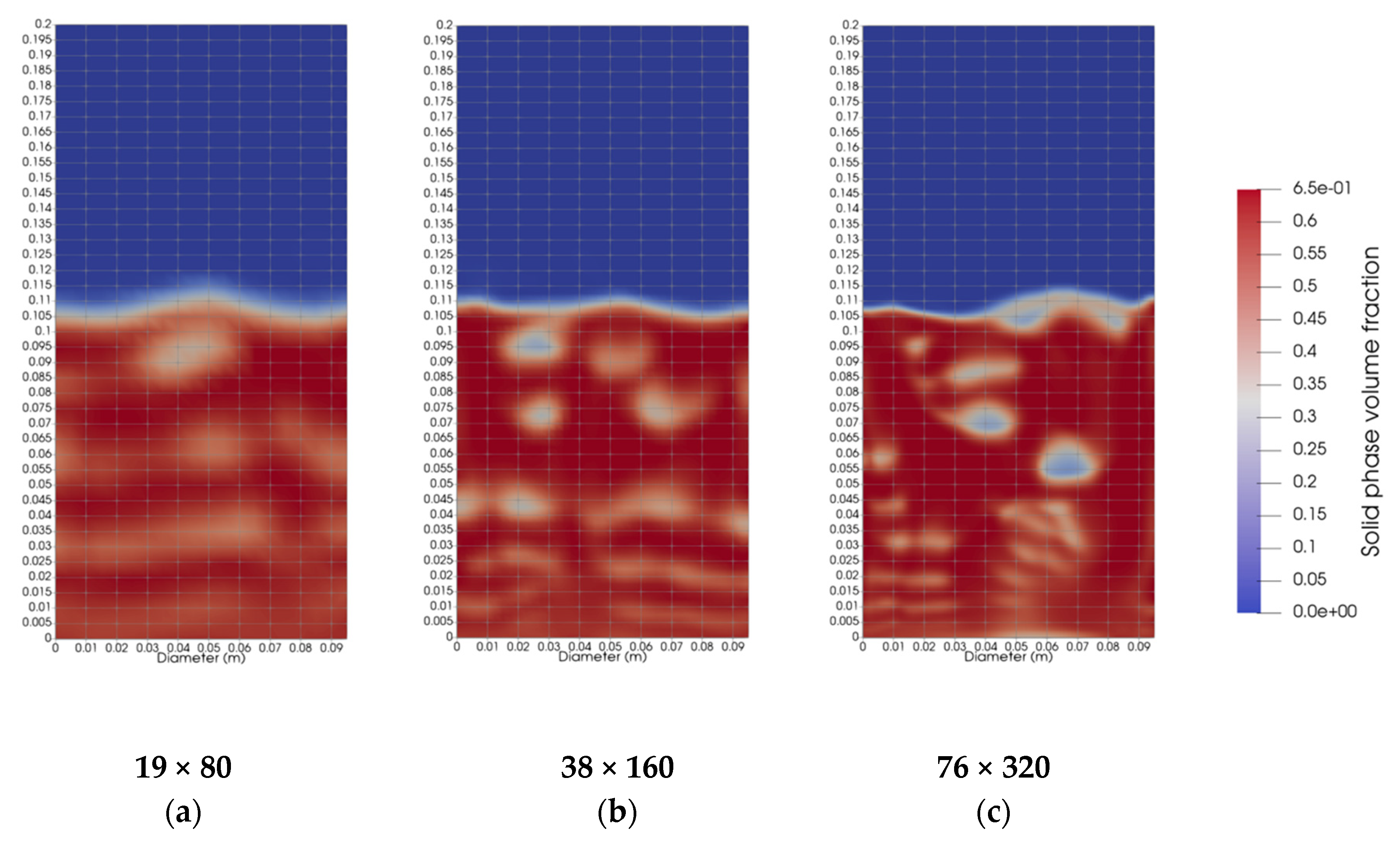
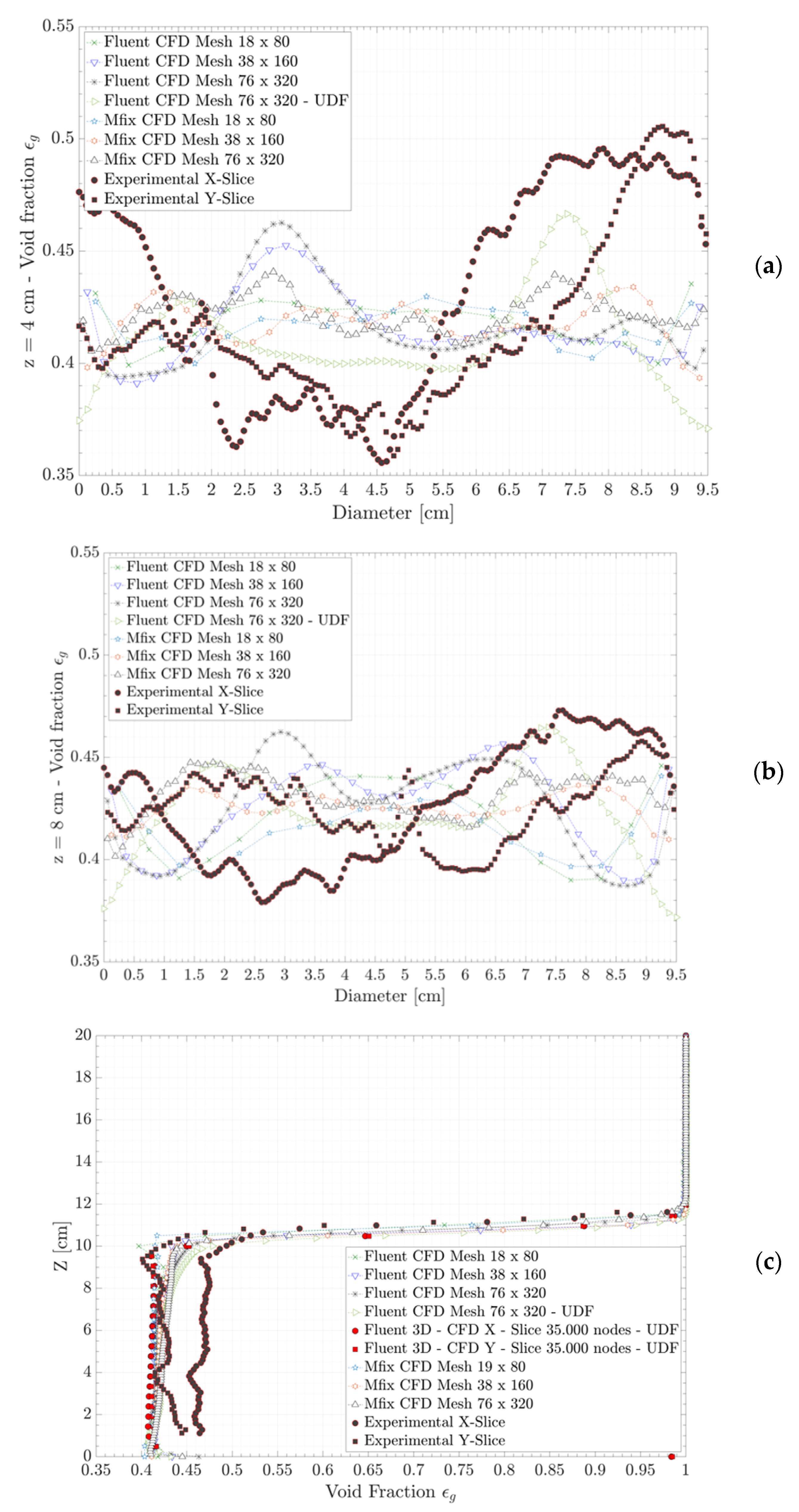
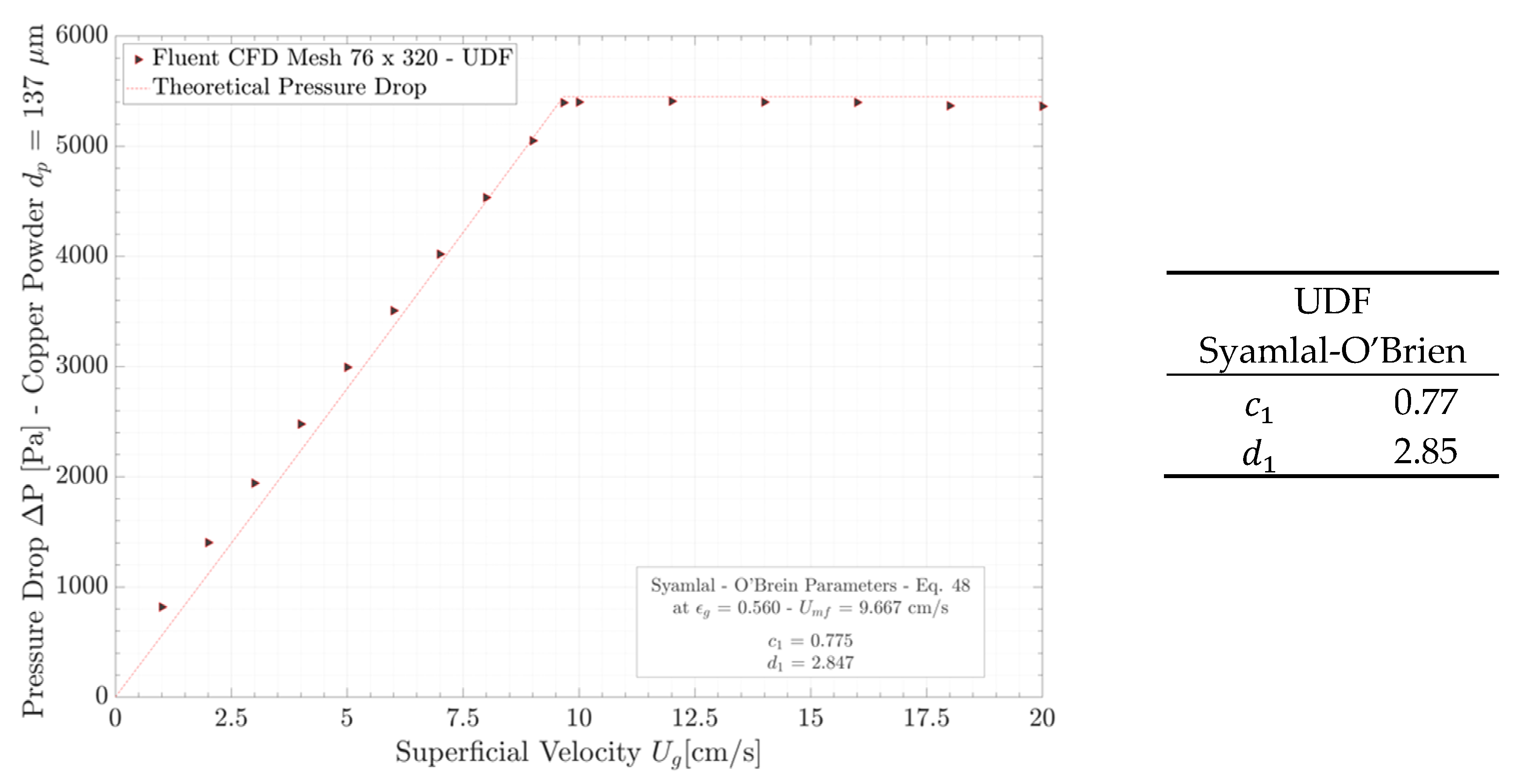
3.1. Numerical Benchmark

In this study, mathematical model was experimentally validated by using data available by Deza et al. [43] which conducted tests on bench scale cold model by the implementation of X-ray methodology. A schematic representation of the apparatus used during tests is shown in Figure 2. In the same figure, characterized properties of particles used as bed material, are also shown. Experiments were carried out by using an acrylic cylindric shaped reactor whose diameter is equal to 9.5 cm. Glass beads were used as bed material (with an initial bed height of 10 cm) and air as fluidizing agent by imposing a superficial gas velocity of $U_g=1.3 ·U_{mf}$. It must be highlighted that bed material used by Deza et al. in their study was different from that identified for the cold model considered here, where copper powder was selected. This methodological choice is justifiable in view of the lack of available experimental data for copper powder. Furthermore, it must be stated that both glass and copper particles are classifiable as Geldart Group B, so that the phenomenological nature of the observations should be the same. This means that mathematical model, parametrized with respect to the different particles used and describing the two processes, should have the same response.

Preliminary experiments were conducted on the ENEA’s ICBFB pseudo-2D cold model, Figure 3; PIV (Particle Image Velocimetry) methodology was adopted to investigate the velocity field structure, seem to confirm these assumptions. A schematic representation of the ICBFB pseudo-2D cold model is shown in Figure 7. Reactor, 10 mm depth in perpendicular direction to the plane, was equipped with a front panel realized in polycarbonate in order to investigate solid motion inside the two chambers. A black back panel was instead used in order to create the right light contrast for the acquisition. The acquisition area was lighted by using two light led sources while a high speed camera, provided by La Vision, was used for frame acquisitions. Cross-correlation method was used to correlate frames at different time in order to solve the solid velocity field. A comparison of two different images of tests conducted, under the same fluidizing conditions, with 0.14 mm copper powder and 0.55 mm glass beads, are shown in Figure 3. The comparison should be regarded as qualitative. Of course, the two experiments were carried out in the same fluidizing conditions but with different density number, in two cases. Nevertheless, the behavior of the two systems appear to be the same. Dimension of the bubbles is in the same order of magnitude. Moreover, bed expansion and up-flowing chamber is visibly less dense than down-flowing one. Furthermore, circulation of bed material through the opening between the two chambers is well visible in the two cases. Under these assumptions, three different grid refinement, by considering as limiting maximum cell size $s_c<10·d_p$, were considered in the ratio 1:0.5:0.125 ($9.10·{\overline{d}}_p$, $4.55·{\overline{d}}_p$ and $2.27·{\overline{d}}_p$) with respect to the coarsest mesh. In such a manner 19 × 80, 38 × 160 and 76 × 320 grid patterns were obtained. Simulations were carried out by imposing for each run, a global simulation time of 40 s with a temporal discretization of 10⁻³ s. Only results between 5 s and 40 s were considered by averaging values every 0.01 s. With the aim to validate computational code, the same mathematical model was also solved by using Mfix code by NETL. A User Defined Function (UDF) was used to modify the original computational code and to implement the parametric model of Syamlal-O’Brien for the calculation of the interphase exchange coefficient. A comparison between theoretical (Ergun equation), experimental and numerical (CFD) pressure drop trough the bed as function of the gas superficial velocity, is shown in Figure 4. Additionally, collected numerical parameters for the UDF definition $c_1$ and $d_1$, calculated by using the procedure proposed by Syamlal et al. [40], are shown in Figure 4.

As it is possible to see, numerical case labelled as Fluent CFD 76 × 320 Mesh–UDF, implementing UDF, fits very well theoretical (red dashed line) and experimental data (red circle). The implemented model provides a good estimation of both minimum fluidization velocity and the correlated pressure drop. Only a slight underestimation and overestimation respect to experimental data (below and above the minimum fluidization velocity value), were registered. Other numerical cases (Fluent without UDF and MFix) only well predict pressure drop above the minimum fluidization conditions. A comparison between CFD solid phase volume fraction obtained by calculations carried out by using different grid refinement, is shown in Figure 5. Images are referred to calculations at simulation time t = 20 s by using Fluent code implementing UDF. As noticeable, coarsest mesh (19 × 80) does not allows to describe with sufficient details, spatial distribution of bubbles as well as their dimensions and borders. Only bed expansion is sufficiently predicted. On the contrary finer meshes (both 38 × 160 and 76 × 320), well describe, with about the same level of detail, bubbles distribution inside the bed, their borders and dimensions: bubble size at bed surface was estimated to be in the order of 2–4 cm whose values are in good agreement with theoretical 0-D solutions (calculations carried out by using correlations whose results are independent from model dimensions). Furthermore, in the case of 76 × 320 grid refinement, visual accordance with X-ray radiography images, obtained by Deza et al. [44] at the same time, is very good.

A comparison between experimental and numerical (CFD) profiles of the void of fraction at different height above the flow distribution plate (z = 4 cm and z = 8 cm), as function of column diameter and column height, is proposed in Figure 6. In the diagrams, experimental data are collected with reference to two perpendicular directions (X-slice and Y-slice). As is evident, numerical and experimental trends are comparable provided finest meshes are considered for both codes here used (Fluent and Mfix). Different proposed profiles in Figure 6a are different in both trend and range. Most probably, the differences between the two groups of curves (theoretical and experimental) are imputable to the real reactor set-up. In particular, the large oscillation in values at z = 4 cm is related to the presence of the flow distribution plate that, in the real reactor, has a finite number of holes through which fluidizing flow is introduced. Furthermore, a channeling phenomenon near the reactor walls is evident so that a greater range of values in the pressure profile at the base of reactor, is registered.

All this promote a not uniform distribution of the flow inside the chamber with the formation of large bubbles where local conditions are favorable. This is not evident in numerical case (CFD) where a uniform distribution of flow at the reactor base was imposed. The observed phenomenon is less evident at z = 8 cm, Figure 6b, because of the greater distance from the flow distributor. Noticeable is, in all cases considered, the slightly differences with respect to experimental X-slice curves even if 3-D solutions are considered, Figure 6c.

Nevertheless, the maximum percentage error is less than 3.5% (coarsest Mfix mesh). The independence of results toward grid refinement was evaluated following ASME (American Society of Mechanical Engineers) procedure for estimation of the uncertainty due to discretization in CFD applications [45]. GCI procedure (grid convergence method), based on the Richardson extrapolation method, was used to evaluate the selected variables (for the purpose: pressure drop through the bed and mean void fraction at z = 4 cm and z = 8 cm) do not exhibit a monotone dependence toward grid refinement.

3.2. ENEA’s ICBFB Cold Model Analysis

The validated numerical code was then applied to study the behavior of the cold model describing the ENEA’s ICBFB. A schematic representation of the cold model considered here is shown in Figure 7. Furthermore, the main properties of the material used (copper powder) for describing the inert fluidizing bed and fluidizing conditions imposed at the inlet section of the two flowing chambers, are shown in the same figure.

Fluid dynamics similarity conditions (Table 1) impose to use as bed material, copper powder with mean particle diameter equal to $d_p=137 \mathsf{\mu }\mathrm{m}$. Of such particles, no fluidizing properties are experimentally known. For the purpose, minimum fluidization conditions were determined by using the correlation proposed by Coltters et al. [46]:

$$U_{mf}=\left(4.7673·{10}^{-6}\right)·X^{0.71635 \pm 0.02213} \mathrm{where} X=\frac{d_p^2·\left({\rho }_s-{\rho }_g\right)}{\mu }{\left(\frac{{\rho }_s}{{\rho }_g}\right)}^{1.23}$$

(26)

whose values are in good agreement with experimental determinations ($R=0.990$) and suitable for particles with diameter $3 \mathsf{\mu }\mathrm{m} \le d_p \le 900 \mathsf{\mu }\mathrm{m}$ and density $2.7\frac{\mathrm{g}}{\mathrm{c}{\mathrm{m}}^3}\le {\rho }_p \le 11.3\frac{\mathrm{g}}{\mathrm{c}{\mathrm{m}}^3}$. The above correlation was successfully tested with experimental data by Chiba et al. [47] considering reference values for copper shot of diameter $d_p=163 \mathsf{\mu }\mathrm{m}$. CFD calibration curve implementing Syamlal-O’Brien parameters for the considered particles is shown in Figure 8. As is possible to see, CFD numerical results are in good accordance with theoretical ones and accurately predict both minimum fluidization velocity (9.67 cm/s) and pressure drop at incipient fluidization conditions (5448.57 Pa).

Main CFD numerical results for the analyzed case are reported in

Table 2. Main numerical results related to CFD analysis of the ENEA’s cold model reactor.

Parameters	Value
$\mathrm{DFB} \mathrm{bed} \mathrm{density}, {\rho }_{DFB mf}$ (kg/m3)	4109.48
$\mathrm{UFB} \mathrm{bed} \mathrm{density}, {\rho }_{UFB mf}$ (kg/m3)	3550.60
$\mathrm{Mean} \mathrm{void} \mathrm{of} \mathrm{fraction} \mathrm{at} \mathrm{vertical} \mathrm{DFB} \mathrm{centerline}, {\epsilon }_{g DFB V}$	0.47
$\mathrm{Mean} \mathrm{void} \mathrm{of} \mathrm{fraction} \mathrm{at} \mathrm{vertical} \mathrm{UFB} \mathrm{centerline}, {\epsilon }_{g UFB V}$	0.52
$\mathrm{Mean} \mathrm{void} \mathrm{of} \mathrm{fraction} \mathrm{at} \mathrm{horizontal} \mathrm{DFB} \mathrm{centerline}, {\epsilon }_{g DFB H}$	0.49
$\mathrm{Mean} \mathrm{void} \mathrm{of} \mathrm{fraction} \mathrm{at} \mathrm{horizontal} \mathrm{UFB} \mathrm{centerline}, {\epsilon }_{g UFB H}$	0.60
$\mathrm{Mean} \mathrm{DFB} \mathrm{chamber} \mathrm{void} \mathrm{of} \mathrm{fraction}, {\epsilon }_{g DFB }$	0.49
$\mathrm{Mean} \mathrm{UFB} \mathrm{chamber} \mathrm{void} \mathrm{of} \mathrm{fraction}, {\epsilon }_{g DFB}$	0.56
$\mathrm{DFB} \mathrm{bubbles} \mathrm{fraction}, {}_{DFB}$	0.18
$\mathrm{UFB} \mathrm{bubbles} \mathrm{fraction}, {}_{UFB}$	0.29
$\mathrm{DBF} \mathrm{bed} \mathrm{Expansion}, H/H_0$	1.13
$\mathrm{UFB} \mathrm{bed} \mathrm{Expansion}, H/H_0$	1.34
$\mathrm{DFB} \mathrm{mean} \mathrm{velocity} \mathrm{at} \mathrm{centerline}, U_{y DFB}$ (m/s)	−0.039
$\mathrm{UFB} \mathrm{mean} \mathrm{velocity} \mathrm{at} \mathrm{centerline}, U_{y UFB}$ (m/s)	0.19
$\mathrm{Pressure} \mathrm{drop} \mathrm{through} \mathrm{opening}, P_{CFD}$ (Pa)	22.390
$\mathrm{CFD} \mathrm{mass} \mathrm{flow} \mathrm{rate} \mathrm{through} \mathrm{opening}, G_{o CFD}$ (kg/s)	5.80
Th. (Equation (6), Kuramoto et al. [19]$), G_{o, th}$ (kg/s)	6.86
Th. (Equation (14b), Kuramoto et al. [19]$), G_{o, th}$ (kg/s)	4.29

where other than main bed properties, also calculated mass flow rate through the opening is proposed. The proposed numerical results are related to the best grid refinement at solution convergence. This latter was evaluated by following the ASME procedure [45] based on the Richardson extrapolation method. In the same table, also theoretical mass flow rate through the opening, evaluated as proposed by Kuramoto et al. [19], were considered for comparison purpose. In this way, two different correlations were used to evaluate numerically the mass flux through the opening connecting the two different regions of the bubbling fluidized bed. The first one, proposed by Jones and Devidson [19], is suitable for small opening ratio $\frac{S_0}{S_d}$:

$$W_d=C_s\frac{S_0}{S_d}\sqrt{2·{\rho }_d·\Delta P_0}$$

(27)

where $S_0$ is the opening section, $S_d$ the downflowing chamber cross sectional area, ${\rho }_d$ the DFB bed density, $\Delta P_0$ the pressure drop across the opening, and $C_s$ a particle discharge coefficient ranging between 0.5 and 0.65. The second correlation here used, was that proposed by Kuramoto et al. [19]:

$$W_d=C_{s0}{\epsilon }_u^{2.35}\sqrt{2·{\rho }_d·\Delta P_0}$$

(28)

where $C_{s0}$ is the discharge coefficient evaluated at ${\epsilon }_u=1$ and equal to 0.5. It must be highlighted that in the above correlations, $W_d$ is the mass flux $[\mathrm{kg}/{\mathrm{m}}^2\mathrm{s}]$ calculated at the mid-section of the downflowing chamber, so that its value is greatly influenced by the real geometry of the reactor. This condition explains the slightly difference between the calculated values and CFD one.

By analyzing numerical results, it is clearly evident as the two regions inside the reactor (UFB and DFB), are characterized by a different behavior. This is well noticeable by evaluating for each of these the bed expansions ratio, the bubbles fraction and the mean void fraction terms. DFB chamber is denser than UFB one, that also exhibits a greater bed expansion respect to the initial condition. Furthermore, a greater fraction of bubbles was observed in the UFB region, where also a positive value (in direction + y) of the mean solid velocity was registered.

On the contrary DFB region is characterized by a negative (in direction-y) value of the same term of velocity. Again, the flux vector evaluated on the opening plane, exhibits as its main component that one in perpendicular direction to the plane along the positive x axes. All these conditions clearly are explained by a motion of the bed material between the two regions inside the reactor from the denser to less dense chamber across the opening at the bottom side of the vertical plate. All the above considerations are well visible in Figure 9, where a comparison between results obtained with the coarsest and finest mesh is proposed for different simulation time. Images show, on the background, the solid phase volume fraction and, in overlapping, the solid phase velocity field. Each of these, clearly shows the bed motion between the two reactor regions. Two different macro-motions are well discernable: the first one (MM1) in counter clockwise direction, that developing along the reactor walls, involves both chambers and, the second one (MM2) concerning only DFB chamber. This latter is composed by two sub-motions: the first one (SM1) identifiable at the bottom left side of the DFB chamber near the flow distributor and, the second (SM2) well visible at the upper right side near the vertical plate. SM1 develops in counter clockwise direction and involves the left side region of the DFB chamber. The closed pathways outlined by this could be responsible of the formation of stagnation regions where reacting material (e.g., char particles) or residual ashes could be trapped causing hot spots or agglomerates. When this motion involves the upper bed surface (left upper area), finer particles like ashes mixed to fine char, could be elutriated and trapped near the reactor wall. Both these are dangerous conditions that must be avoided in order to not compromise the operating functionality of the reactor. SM2, instead, involves the right region of the DFB chamber in clockwise direction. It develops from the bottom surface of the chamber toward the upper bed surface where its motion is inverted. A descending solid flow near the vertical plate wall, is originated that drags solid material toward the opening at the bottom side of the plate. Here solid materials are mixed to that from MM1, that crossing the opening, enters the UFB chamber.

Entering materials are then vigorously transported by the ascending gas flow toward the surface of the bed where they are reintroduced in the down flowing chamber. Comparing bed structures resulting from the solution of the mathematical model with the two different grid refinements, it is noticeable as the coarsest mesh can’t capture with good level of detail smallest formation inside the bed. Moreover, bubbles distribution and their dimensions cannot be evaluated with sufficient grade of precision. Only bed expansion and main solid flow macro-motions are sufficiently predicted by coarse mesh. A comparison between results obtained by using the two levels of refinement are shown in Figure 9. In the proposed diagrams, velocity and void fraction profiles are compared. Circulation of the bed material between the two zones of the reactor is also confirmed by the velocity profiles, Figure 10. As shown UFB profiles exhibit mean positive values of velocity at the contrary of DFB ones whose mean values are negative. By the same diagram also the inversion of solid flows near the reactor walls are visible. Furthermore, UFB velocity profiles are shifted toward the wall of the vertical plate where the formation of bubbles of greater dimensions is promoted.

This latter condition is well confirmed by the analysis of the distribution of the void fraction along the chamber, Figure 11a,c. At least, comparing void fraction profiles as function of the bed height, Figure 11b,c, it can be observed that UFB chamber exhibits a greater bed expansion than DFB one and how this latter is denser than the first one. In brief, comparing results, it can be stated that coarsest mesh over predict velocity of about 45% and void fraction of about 4% are well compared with fine mesh (values at convergence). A visual representation of 3D–CFD solution at simulation time t = 10 s, is proposed in Figure 12, where solid phase volume fraction and solid velocity field on main section planes of the reactor are shown. X–Y slicing plane, shows well the distribution of the field velocity in the two chambers, Figure 12a, while granular solid phase iso-surfaces depicted in 12b, delimitate bubbles formations inside the reactor. This latter image confirms general phenomenon discussed above. Bubbles of dimensions in the order of 4–6 cm, mainly develop in UFB chamber near the wall surfaces of the vertical plate by-passing, in this region, reacting flows. The evaluated mass flow rate across the opening, in 3D-CFD simulation, equal to ${\displaystyle \oint }{\mathrm{W}}_{\mathrm{x}}d{A}_O=6.65 \mathrm{kg}/\mathrm{s}$, is comparable both with 2D and theoretical results proposed in Table 2. In order to investigate the recirculation time of solids inside the reactor, char particles by biomass gasification, were considered. Experimentally measured density of char particles was evaluated to be equal to ${\rho }_p=975 \mathrm{kg}/{\mathrm{m}}^3$. Five values of diameter ranging from 0.2 mm to 1.0 mm were considered as average diameter of char particles in the bed, as result of primary fragmentation and particle shrinkage. These values can be correlated to the original fuel size (mother fuel particle) as proposed by Gómez et al. [48].

As proposed by the authors, the initial fuel size $d_f$, is related to the average size of char particle inside the bed, $d_{ch,b}$, by the following correlation:

$$\frac{d_{ch,b}}{d_f}\approx {\left(\frac{\phi }{n_1{n}_{2,m}}\right)}^{\frac{1}{3}}\sigma$$

(29)

where $\phi$ is the shrinkage factor, $n_1$ the number of fragments, $n_{2,m}$ and $\sigma$ multiplication factors determined, experimentally. Experimental determinations proposed by the same authors indicate for wood chips a value of $\frac{d_{ch,b}}{d_f}=0.34$, which was assumed here as reference for numerical evaluations.

Table 3. Similarity of fluid dynamic for char particles inside cold model.

	Particles
	${\overline{\mathit{d}}}_{\mathit{p}}=0.80 \mathbf{m}\mathbf{m}$		${\overline{\mathit{d}}}_{\mathit{p}}=1.00 \mathbf{m}\mathbf{m}$
	Char Real	Cold Model	Char Real	Cold Model
$\mathrm{Fluidizing} \mathrm{flow} \mathrm{density}, {\rho }_g$ (kg/m3)	0.33	0.99	0.33	0.99
Fluidizing flow viscosity, µ (Pa s)	4.38 × 10−5	1.89 × 10−5	4.38 × 10−5	1.89 × 10−5
$\mathrm{Particle} \mathrm{density},$ (kg/m3)	975	2937	975	2937
$\mathrm{Archimedes} \mathrm{number}, Ar$	8.38 × 102		1.64 × 103
$\mathrm{Reynolds} \mathrm{number}, Re$	1.19		2.21
$\mathrm{Froude} \mathrm{number}, Fr$	2.23 × 104		2.98 × 104
$\mathrm{Density} \mathrm{number}, De$	3.37 × 10−4		3.37 × 10−4
$\mathrm{Minimum} \mathrm{fluidization} \mathrm{velocity}, U_{mf}$ (cm/s)	19.80	10.36	29.49	15.43
$\mathrm{Terminal} \mathrm{velocity}, U_t$ (m/s)	0.64	0.33	1.13	0.59
$\mathrm{Particle} \mathrm{diameter}, {\overline{d}}_p$ (mm)	0.80	0.22	1.00	0.27
$\mathrm{Length} \mathrm{scale} \mathrm{ratio}, Le-d_{p GR}/d_{p CM}$	3.65
$\mathrm{Gas} \mathrm{flow} \mathrm{velocity} \mathrm{ratio}, Fl$$-(U_{GR}/U_{CM}$)	1.91
$\mathrm{Gas} \mathrm{flow} \mathrm{rate} \mathrm{ratio}, (Q_{GR}/Q_{CM}$)	25.49
$\mathrm{Time} \mathrm{ratio}, (t_{GR}/t_{CM}$)	1.91

summarizes the scaling parameters used to study the behavior of char particles inside the cold model reactor. The table present data related to char particles of size 0.80 mm and 1.00 mm, respectively. The only ones whose results were considered of interest.

3D numerical simulations were carried out by setting up a DDPM as above discussed. Five equivalent particles were injected at simulation time t = 10 s when inert bed material was well fluidized. Simulations were terminated at simulation time t = 20 s and data about particles (e.g., position, velocity, and momentum) were collected every 0.01 s. Results showed that particles whose diameter is lesser than 0.22 mm (equivalent to 0.80 mm char particles), segregate on bed surface in the upper left region of the bed, near the reactor walls, where stagnant fluid dynamic conditions are encountered. Instead, particles whose diameter is in the range 0.22 mm to 0.27 mm (equivalent to 1.00 mm char particles) well follow bed motion, circulating between the two reaction chambers.

The calculated recirculation time of average particles is in the order of 5 s for 0.22 mm particle, and 6–7 s for 0.27 mm particle, well comparable with the average bed recirculation time estimated to be in the order of 6–7 s. 2D-images of particle motion inside the reactor bed are shown in Figure 13, where white and black dots are used to identify respectively 0.22 mm and 0.27 mm particles. As shown particle of averaged size 0.22 mm, follows the main bed macro-motion, circulating continuously between the chambers, while 0.27 mm particle, seems to be trapped in the bottom section of the UFB chamber where closed pathway solid flow lines are encountered. All these conditions suggest, in last instance, the dimension of fuel particles that must be used in the real reactor to avoid both segregation and agglomeration phenomenon. As discussed above, by using the correlations proposed by Gómez et al. [48], these shouldn’t exceed the estimated value of 5–10 mm.

4. Conclusions

In this paper, the hydrodynamic of cold model reactor was investigated numerically in order to get guidelines in the design procedure of a real reactor. CFD method was applied by treating continuous both granular solid phase and gaseous phase. Eulerian–Eulerian multiphase approach was then implemented to describe the two interacting phases while a DDPM was considered to evaluate interactions between continuous phases and solid particles modelling char.

Mathematical model was validated first by using experimental data available in the technical literature and then applied to the numerical case under investigation. The geometry of the ICBFB cold model reactor and the fluidizing conditions were fully defined by applying scaling laws to preserve fluid dynamic similarities between the real pilot reactor at full scale (1 MW_th), operating at high temperature, and that one at bench scale operating at ambient conditions. Behavior of the inert bed material was investigated under the design fluidizing conditions and critical conditions (e.g., elutriation and agglomeration phenomenon) were identified.

Recirculation rate of bed material between the two reaction chambers was also evaluated and compared with theoretical one calculated by using semi-empirical correlations by different authors. The behavior of solid particles modelling char was also investigated by injecting solid particles of different size inside the well fluidized bed and by keeping for each one all information (e.g., position, velocity, and momentum) at different simulation time.

Results indicate that the recirculation time of bed material is in the order of 6–7 s at bench scale and, respectively, of 15–20 s at full scale.

Furthermore, information about solid particles inside the bed that should be used to avoid elutriation and agglomeration phenomenon are achieved. Particles whose dimensions are less than 0.22 mm (0.80 mm at full scale reactor) should segregate on bed surface agglomerating near the reactor walls, while particles greater than 0.27 mm (1.00 mm at full scale reactor) should migrate to the bottom section of the UFB chamber were stagnant fluid dynamic conditions were detected. Particles of dimensions ranging between 0.22 mm and 0.27 mm, instead, well follow the bed motion circulating between the two reaction chambers.

All these information suggest that the dimension of the mother fuel particles, to feed to the real pilot reactor, should not exceed the evaluated value of 5–10 mm.

Results obtained should be considered as preliminary. Further investigations need to be done in order to validate numerical CFD results, experimentally. Developments of the work are devoted to experimental investigations on the ENEA’s pseuo-2D cold model where PIV methodology is implemented to solve the solid velocity field. Moreover, the effects of fluid dynamic implications related to the real bed mixture when both solid fuel particles and inert bed material are considered, need to be investigated further. From numerical point of view, implementation of the chemistry with related kinetics of reaction is the next step.

5. Patents

E. Fanelli, F. Nanna, D. Barisano, G. Cornacchia, G. Braccio. “Reattore per la gassificazione di biomasse” IT Patent n° 202019000004530, issue December 13, 2019.

References

1. IEA. Bioenergy Power Generation; IEA: Paris, France, 2020. [Google Scholar]
2. Demirbas, A. Biofuels sources, biofuel policy, biofuel economy and global biofuel projections. Energy Convers. Manag. 2008, 49, 2106–2116. [Google Scholar] [CrossRef]
3. Devi, L.; Ptasinski, K.J.; Janssen, F.J.J.G. A review of the primary measures for tar elimination in biomass gasification processes. Biomass Bioenergy 2003, 24, 125–140. [Google Scholar] [CrossRef]
4. Santos, R.G.D.; Alencar, A.C. Biomass-derived syngas production via gasification process and its catalytic conversion into fuels by Fischer Tropsch synthesis: A review. Int. J. Hydrogen Energy 2019. [Google Scholar] [CrossRef]
5. Jiang, G.; Wei, L.; Chen, Z.; Peng, L.; He, N.; Wu, C. Experimental Investigation of Particle Circulation in an Internally Circulating Clapboard-Type Fluidized Bed. Chem. Eng. Technol. 2020, 43, 253–262. [Google Scholar] [CrossRef]
6. Basu, P. Combustion and Gasification in Fluidized Beds; CRC Press: Boca Raton, FL, USA, 2006; ISBN 9780429075018. [Google Scholar]
7. Abba, I.A.; Grace, J.R.; Bi, H.T.; Thompson, M.L. Spanning the flow regimes: Generic fluidized-bed reactor model. AIChE J. 2003, 49, 1838–1848. [Google Scholar] [CrossRef]
8. Alauddin, Z.A.B.Z.; Lahijani, P.; Mohammadi, M.; Mohamed, A.R. Gasification of lignocellulosic biomass in fluidized beds for renewable energy development: A review. Renew. Sustain. Energy Rev. 2010, 14, 2852–2862. [Google Scholar] [CrossRef]
9. Hofbauer, H. Biomass CHP plant Guessing—A success story. Pyrolysis Gasif. Biomass Waste 2003, 371–383. [Google Scholar]
10. Bolhar-Nordenkampf, M.; Hofbauer, H.; Rauch, R.; Tremmel, H.; Aichernig, C. Biomass CHP Plant Güssing–Using Gasification for Power Generation. In Proceedings of the 2nd regional Conference on Energy Technology Towards a Clean Envionnment, Phuket, Thailand, 12–14 February 2003. [Google Scholar]
11. Kern, S.; Pfeifer, C.; Hofbauer, H. Gasification of wood in a dual fluidized bed gasifier: Influence of fuel feeding on process performance. Chem. Eng. Sci. 2013, 90, 284–298. [Google Scholar] [CrossRef]
12. Karl, J.; Pröll, T. Steam gasification of biomass in dual fluidized bed gasifiers: A review. Renew. Sustain. Energy Rev. 2018, 98, 64–78. [Google Scholar] [CrossRef]
13. Woolcock, P.J.; Brown, R.C. A review of cleaning technologies for biomass-derived syngas. Biomass Bioenergy 2013, 52, 54–84. [Google Scholar] [CrossRef]
14. Valderrama Rios, M.L.; González, A.M.; Lora, E.E.S.; Almazán del Olmo, O.A. Reduction of tar generated during biomass gasification: A review. Biomass Bioenergy 2018, 108, 345–370. [Google Scholar] [CrossRef]
15. Guan, G.; Kaewpanha, M.; Hao, X.; Abudula, A. Catalytic steam reforming of biomass tar: Prospects and challenges. Renew. Sustain. Energy Rev. 2016, 58, 450–461. [Google Scholar] [CrossRef] [Green Version]
16. Singh, R.I.; Brink, A.; Hupa, M. CFD modeling to study fluidized bed combustion and gasification. Appl. Eng. 2013, 52, 585–614. [Google Scholar] [CrossRef]
17. Ariyaratne, W.K.H.; Manjula, E.V.P.J.; Ratnayake, C.; Melaaen, M.C. CFD Approaches for Modeling Gas-Solids Multiphase Flows–A Review. In Proceedings of the 9th EUROSIM Congress on Modelling and Simulation, EUROSIM 2016, The 57th SIMS Conference on Simulation and Modelling SIMS 2016, Oulu, Finland, 12–16 September 2016; 2016. [Google Scholar] [CrossRef] [Green Version]
18. Kuramoto, M.; Furusawa, T.; Kunii, D. Development of a new system for circulating fluidized particles within a single vessel. Powder Technol. 1985, 44, 77–84. [Google Scholar] [CrossRef]
19. Kuramoto, M.; Kunii, D.; Furusawa, T. Flow of dense fluidized particles through an opening in a circulation system. Powder Technol. 1986, 47, 141–149. [Google Scholar] [CrossRef]
20. Felice, R.D.I.; Rapagna, S.; Foscolo, P.U. Cold modelling studies of fluidized bed reactors. Chem. Eng. Sci. 1992, 47, 2233–2238. [Google Scholar] [CrossRef]
21. Niewland, J.J.; Huizenga, P.; Kuipers, J.A.M.; van Swaaij, W.P.M. Hydrodynamic modelling of circulating fluidised beds. Chem. Eng. Sci. 1994, 49, 5803–5811. [Google Scholar] [CrossRef] [Green Version]
22. Zimmermann, S.; Taghipour, F. CFD Modeling of the Hydrodynamics and Reaction Kinetics of FCC Fluidized-Bed Reactors. Ind. Eng. Chem. Res. 2005, 44, 9818–9827. [Google Scholar] [CrossRef]
23. Foscolo, P.U.; Germanà, A.; Jand, N.; Rapagnà, S. Design and cold model testing of a biomass gasifier consisting of two interconnected fluidized beds. Powder Technol. 2007, 173, 179–188. [Google Scholar] [CrossRef]
24. Papadikis, K.; Bridgwater, A.V.; Gu, S. CFD modelling of the fast pyrolysis of biomass in fluidised bed reactors, Part A: Eulerian computation of momentum transport in bubbling fluidised beds. Chem. Eng. Sci. 2008, 63, 4218–4227. [Google Scholar] [CrossRef]
25. Papadikis, K.; Gu, S.; Bridgwater, A.V. CFD modelling of the fast pyrolysis of biomass in fluidised bed reactors. Part B. Heat, momentum and mass transport in bubbling fluidised beds. Chem. Eng. Sci. 2009, 64, 1036–1045. [Google Scholar] [CrossRef]
26. Papadikis, K.; Gu, S.; Bridgwater, A.V. A CFD approach on the effect of particle size on char entrainment in bubbling fluidised bed reactors. Biomass Bioenergy 2010, 34, 21–29. [Google Scholar] [CrossRef] [Green Version]
27. Pecate, S.; Morin, M.; Kessas, S.A.; Hemati, M.; Kara, Y.; Valin, S. Hydrodynamic study of a circulating fluidized bed at high temperatures: Application to biomass gasification. Kona Powder Part. J. 2019, 36, 271–293. [Google Scholar] [CrossRef]
28. Armstrong, L.M.; Luo, K.H.; Gu, S. Two-dimensional and three-dimensional computational studies of hydrodynamics in the transition from bubbling to circulating fluidised bed. Chem. Eng. J. 2010, 160, 239–248. [Google Scholar] [CrossRef]
29. Gerber, S.; Behrendt, F.; Oevermann, M. An Eulerian modeling approach of wood gasification in a bubbling fluidized bed reactor using char as bed material. Fuel 2010, 89, 2903–2917. [Google Scholar] [CrossRef]
30. Liu, H.; Elkamel, A.; Lohi, A.; Biglari, M. Computational fluid dynamics modeling of biomass gasification in circulating fluidized-bed reactor using the eulerian-eulerian approach. Ind. Eng. Chem. Res. 2013, 52, 18162–18174. [Google Scholar] [CrossRef]
31. Canneto, G.; Freda, C.; Braccio, G. Numerical simulation of gas-solid flow in an interconnected fluidized bed. Science 2015, 19, 317–328. [Google Scholar] [CrossRef]
32. Barisano, D.; Canneto, G.; Nanna, F.; Alvino, E.; Pinto, G.; Villone, A.; Carnevale, M.; Valerio, V.; Battafarano, A.; Braccio, G. Steam/oxygen biomass gasification at pilot scale in an internally circulating bubbling fluidized bed reactor. Fuel Process. Technol. 2016, 141, 74–81. [Google Scholar] [CrossRef]
33. Barisano, D.; Canneto, G.; Nanna, F.; Villone, A.; Alvino, E.; Carnevale, M.; Pinto, G. Production of Gaseous Carriers Via Biomass Gasification for Energy Purposes. Energy Procedia 2014, 45, 2–11. [Google Scholar] [CrossRef] [Green Version]
34. Glicksman, L.R.; Hyre, M.; Woloshun, K. Simplified scaling relationships for fluidized beds. Powder Technol. 1993, 77, 177–199. [Google Scholar] [CrossRef]
35. Kolar, A.K.; Leckner, B. Scaling of CFB boiler hydrodynamics. In Proceedings of the 1st National Con-ference on Advances in Energy Research (AER 2006), Mumbai, India, 4–5 December 2006; pp. 34–40. [Google Scholar]
36. Wen, C.Y.; Yu, Y.H. A generalized method for predicting the minimum fluidization velocity. AIChE J. 1966, 12, 610–612. [Google Scholar] [CrossRef]
37. Syamlal, M.; O’Brien, T.J. Computer Simulation of Bubbles in a Fluidized Bed. AIChE Symp. Ser. 1989, 85, 22–31. [Google Scholar]
38. Gidaspow, D. Continuum and kinetic theory descriptions. In Multiphase Flow and Fluidization; Academic Press: Cambridge, MA, USA, 1994; ISBN 9780080512266. [Google Scholar]
39. Taghipour, F.; Ellis, N.; Wong, C. Experimental and computationa l study of gas-solid fluidized bed hydrodynamics. Chem. Eng. Sci. 2005. [Google Scholar] [CrossRef]
40. Syamlal, M.; Brien, T.O. The Derivation of a Drag Coefficient Formula from Velocity-Voidage Correlations; Technical Note; US Department of energy, Office of Fossil Energy, NETL: Morgantown, WV, USA, 1994.
41. Lun, C.K.K.; Savage, S.B.; Jeffrey, D.J.; Chepurniy, N. Kinetic theories for granular flow: Inelastic particles in Couette flow and slightly inelastic particles in a general flowfield. J. Fluid Mech. 1984. [Google Scholar] [CrossRef]
42. Theory Guide: Ansys Fluent 15.0; ANSYS-INC.: Canonsburg, PA, USA, 2013.
43. Ponti, G.; Palombi, F.; Abate, D.; Ambrosino, F.; Aprea, G.; Bastianelli, T.; Beone, F.; Bertini, R.; Bracco, G.; Caporicci, M.; et al. The role of medium size facilities in the HPC ecosystem: The case of the new CRESCO4 cluster integrated in the ENEAGRID infrastructure. In Proceedings of the 2014 International Conference on High Performance Computing and Simulation, Bologna, Italy, 21–25 July 2014; pp. 1030–1033. [Google Scholar]
44. Deza, M.; Franka, N.P.; Heindel, T.J.; Battaglia, F. CFD modeling and X-ray imaging of biomass in a fluidized bed. J. Fluids Eng. Trans. Asme 2009, 131, 1113031–11130311. [Google Scholar] [CrossRef]
45. Division, F.E.; Statement, E.P.; Accuracy, N.; Eng, A.J.F.; Engineering, F.; Policy, E.; Accuracy, N.; Eng, A.J.F. Procedure for Estimation and Reporting of Uncertainty Due to Discretization in CFD Applications. J. Fluids Eng. Trans. ASME 2008, 130, 2008–2011. [Google Scholar] [CrossRef] [Green Version]
46. Coltters, R.; Rivas, A.L. Minimum fluidation velocity correlations in particulate systems. Powder Technol. 2004, 147, 34–48. [Google Scholar] [CrossRef]
47. Chiba, S.; Chiba, T.; Nienow, A.W.; Kobayashi, H. The minimum fluidisation velocity, bed expansion and pressure-drop profile of binary particle mixtures. Powder Technol. 1979, 22, 255–269. [Google Scholar] [CrossRef]
48. Gómez-Barea, A.; Leckner, B. Modeling of biomass gasification in fluidized bed. Prog. Energy Combust. Sci. 2010, 36, 444–509. [Google Scholar] [CrossRef]
Figure 1. ENEA’s 1 MWth Internally Circulating Bubbling Fluidized Bed (ICBFB) pilot plant: (a) Gasifier details; (b) Whole pilot plant layout: it is visible the biomass feeding system, the gasifier, the heat exchanger and the syngas cleaning system.
Processes 08 01323 g001
Figure 2. Schematic representation of the experimental apparatus used by Deza et al. [44], considered for the numerical validation of the mathematical model. In the table, characterizing properties of solid particles composing the inert bed material are collected.
Processes 08 01323 g002
Figure 3. ENEA’s ICBFB pseudo-2D cold model test ring implementing LaVision PIV system for velocity field evaluations. Images of test conducted with: (a) 0.14 mm copper powder particles; (b) 0.55 mm glass beads.
Processes 08 01323 g003
Figure 4. Pressure drop through the bed as function of the superficial gas velocity: comparison between theoretical pressure drop (red dashed line), experimental (red dot), and CFD calculation (black triangle). CFD calculations were obtained by implementing the parametric model of Syamlal-O’Brien: parameters of this model, are shown in the table.
Processes 08 01323 g004
Figure 5. Instantaneous solid phase volume fraction at time t = 20 s: images are referred to calculations carried out by using Fluent code implementing user defined function (UDF) considering three different grid refinement: (a) 19 × 80; (b) 38 × 160; (c) 76 × 320.
Processes 08 01323 g005
Figure 6. Averaged void fraction profiles as function of column diameter at (a) 4 cm and (b) 8 cm above flow distribution plate; (c) function of column height (calculated as mean values of all grids at the same height). Comparison between experimental and numerical data averaged between 5 s and 40 s.
Processes 08 01323 g006
Figure 7. Schematic representation of the cold model used to investigate the hydrodynamic behavior of the ENEA’s ICBFB reactor. In the table, characterizing properties of solid particles composing the inert bed material and fluidizing condition for the two chambers are collected.
Processes 08 01323 g007
Figure 8. Pressure drop through the bed as function of the superficial gas velocity: comparison between theoretical pressure drop (red dashed line) and CFD calculation (black triangle). CFD calculations were obtained by implementing the parametric model of Syamlal-O’Brien: parameters of this model are shown in the table.
Processes 08 01323 g008
Figure 9. Solid phase volume fraction and field velocity comparison between CFD solutions with different grid refinement and at various simulation time.
Processes 08 01323 g009
Figure 10. Main CFD results. Comparison between solutions obtained considering the coarsest and finest mesh: solid phase velocity profiles. Plotted data were averaged over simulation time between 1 s and 20 s.
Processes 08 01323 g010
Figure 11. Main CFD results. Comparison between solutions obtained by considering the coarsest and finest mesh: (a) void fraction profiles at centerline in the two chambers; void fraction profiles as function of the bed height in the down-flowing bed (DFB) (b) and up-flowing bed (UFB) chamber (c). Plotted data were averaged over simulation time between 1 s and 20 s.
Processes 08 01323 g011
Figure 12. 3D-CFD visual representation at simulation time t = 10 s: (a) solid phase volume fraction and solid velocity field visualization on main section planes (colors of arrows are only delimiting the cutting plane where vector field is displayed); (b) granular solid phase iso-surfaces (red ε s = 0.35 , blue ε s = 0.15 ) delimiting bubbles formation inside the two chambers.
Processes 08 01323 g012
Figure 13. Visual representation of equivalent char particles position inside cold model reactor at different simulation time: white dot for particle of diameter d ¯ p = 0.22   mm ; black dot for particle of diameter d ¯ p = 0.27   mm . Images also show the instantaneous granular solid phase volume fraction and the solid velocity field.
Processes 08 01323 g013