Article

A Confidence Interval-Based Process Optimization Method Using Second-Order Polynomial Regression Analysis

1
Electronics and Telecommunications Research Institute, Daegu-Gyeongbuk Research Center, Daegu 42994, Korea
2
Korea Institute of Ceramic Engineering & Technology, Icheon Branch, Engineering Ceramics Center, Icheon-si 17303, Korea
*
Authors to whom correspondence should be addressed.
Processes 2020, 8(10), 1206; https://doi.org/10.3390/pr8101206
Submission received: 28 August 2020 / Revised: 18 September 2020 / Accepted: 19 September 2020 / Published: 24 September 2020
(This article belongs to the Section Process Control and Monitoring)

Abstract

:
In the manufacturing processes, process optimization tasks, to optimize their product quality, can be performed through the following procedures. First, process models mimicking functional relationships between quality characteristics and controllable factors are constructed. Next, based on these models, objective functions formulating process optimization problems are defined. Finally, optimization algorithms are applied for finding solutions for these functions. It is important to note that different solutions can be found whenever these algorithms are independently executed if a unique solution does not exist; this may cause confusion for process operators and engineers. This paper proposes a confidence interval (CI)-based process optimization method using second-order polynomial regression analysis. This method evaluates the quality of the different solutions in terms of the lengths of their CIs; these CIs enclose the outputs of the regression models for these solutions. As the CIs become narrower, the uncertainty about the solutions decreases (i.e., they become statistically significant). In the proposed method, after sorting the different solutions in ascending order, according to the lengths, the first few solutions are selected and recommended for the users. To verify the performance, the method is applied to a process dataset, gathered from a ball mill, used to grind ceramic powders and mix these powders with solvents and some additives. Simulation results show that this method can provide good solutions from a statistical perspective; among the provided solutions, the users are able to flexibly choose and use proper solutions fulfilling key requirements for target processes.

1. Introduction

In manufacturing, one of the major concerns faced by the industry is in saving production costs and time, and at the same time, improving the quality of the products. These can be achieved by optimizing crucial controllable factors (also known as input, process, or design parameters) in target processes [1,2]. To obtain the best values of the controllable factors, we must first formulate functional relationships (i.e., process models) between these factors and quality characteristics; regression analysis and machine learning methods can be used to construct these relationships. After finishing the model-building, objective functions are defined based on the models, and then optimization techniques are applied to these functions to find optimal solutions (also known as optimal recipes).
To build the process models, we prepare a process dataset, composed of input-output observation pairs, beforehand. Experimental designs [3], such as full factorial, central composite, and Box-Behnken designs have been widely employed to collect these datasets in systematic ways. Second-order polynomial regression analysis [2,4,5] is the most popular statistical technique for constructing the process models from the collected datasets; this technique has been successfully used for process optimization in various fields [6,7,8,9,10,11,12,13,14,15]. The advantages of this regression technique can be summarized as follows. First, since the number of levels (i.e., the number of points at which experiments are performed) in each factor, are in general, set as 3 or 4, the second-order polynomial regression models can capture the nonlinearities contained in the process data adequately; as the order of the models become larger than 2, the model complexity (i.e., the number of regression coefficients) exponentially increase, and as a result the resulting models overfit the target datasets. Second, when the input-output relations are described by these models, an output variable is nonlinear in input variables but is linear in the coefficients; one can easily obtain least squares estimates for the unknown coefficients, which are closed-form solutions minimizing residual sum-of-squares. Last, the constructed models, based on the method of least squares, are highly interpretable; by examining the estimated coefficients closely, one can understand which terms affect the output more than the others.
After building the polynomial regression models mimicking the input-output relationships of target processes, one can try to find input values (i.e., the values of controllable factors) that make the model outputs (i.e., quality characteristics) equal to desired values (e.g., maximum, minimum, or target values) through optimization procedures. These models are also capable of predicting the output values corresponding to arbitrary input points at which experiments were not conducted. If the models have a single output and the aim of optimization procedures is to maximize or minimize it, we make use of regression functions themselves as the objective functions. If there are user-defined target values for the output values, one should define the objective functions by modifying the regression functions suitably.
One of the major difficulties encountered in the optimization procedure is that a unique solution may not exist. In particular, when the goal is to find a solution that makes the output values equal to user-defined target values, one cannot find a unique solution. This can be easily confirmed from surfaces of regression functions (also known as response surfaces). In this case, different solutions can be found whenever optimization algorithms are independently executed; this is common to both derivative-based and derivative-free optimization methods. In the derivative-based methods (e.g., numerical optimization methods [16]), if searching the solutions starts at different initial points, discovered solutions may be changed; in the derivative-free methods (e.g., metaheuristics [17]), stochastic mechanisms are employed to find the solutions, and thus different solutions are obtained each time. In summary, as explained above, a unique solution may not exist in process optimization problems, and therefore, different solutions are discovered when running optimization algorithms multiple times; what seems to be lacking is the study to determine which of these different solutions to be selected and then recommended for users, such as process operators and engineers.
In this paper, we propose a confidence interval (CI)-based process optimization method using second-order polynomial regression analysis; it aimed at assessing the quality of the different solutions from a statistical point of view and selecting statistically significant solutions to be provided to the users. The second-order polynomial regression models give us closed-form expressions able to calculate CIs in which the model outputs for the solutions are included. The proposed method uses the length of these CIs as a measure to evaluate the different solutions discovered by optimization techniques; among the different solutions, only a few solutions whose lengths of CIs are shorter than others, are selected and recommended for the users.
To verify the performance, we apply the proposed method to a process dataset collected from a ball mill. In ceramic industries, this equipment has been popularly used to pulverize ceramic powders and to mix these powders with solvents and some additives [18]; finishing the operation of a ball mill, one can obtain a slurry where they are mixed with each other. Among various measurable variables from the slurry, particle size distribution and viscosity have been regarded as key quality characteristics. The focus of this study is limited to the slurry viscosity. Central composite design (CCD) [2,3] is used to prepare the experiment dataset required to construct process models. The purpose of applying the proposed method to the ball mill is to find the values of its controllable factors, achieving the values of slurry viscosity, equal to target values. The importance of achieving its desired values are attributed to the fact that it plays a vital role in a next stage process, i.e., a spray dryer. This is a unit process to produce granules by spray drying the slurry. Therefore, the slurry should satisfy the viscosity values required to obtain high-quality (i.e., uniform and free-flowing) granules [18]. The proposed method is able to recommend several reliable solutions (i.e., the values of controllable factors achieving desired values of slurry viscosity) from a statistical viewpoint. In accordance with practical situations, the users can flexibly choose and use proper solutions among them.
The remainder of this paper is organized as follows. Section 2 explains the second-order polynomial regression method for process modeling, CIs enclosing model outputs, and Monte Carlo (MC)-based method to estimate the importance of controllable factors; one can prioritize these factors according to the estimated importance values, and their priorities can be quite useful for the operations of target processes. Section 3 outlines particle swarm optimization (PSO), one of the widely used global optimization methods, and the proposed CI-based process optimization method; in fact, any optimization methods can be employed in the proposed method. Section 4 describes a target process (i.e., a ball mill) and a process dataset gathered from it via CCD. Section 5 presents the simulation results and discussion, and finally, we give our conclusions in Section 6.

2. Process Modeling Using Second-Order Polynomial Regression

In this section, the second-order polynomial regression analysis and the MC-based method inspired from Ref. [10,19] are explained in detail. From now on, scalars and vectors are written in italics, and bold lowercase, respectively, and matrices are written in bold capitals.

2.1. Second-Order Polynomial Regression Analysis

The 2nd-order polynomial regression models describe the functional relationships between p input variables (also called independent, explanatory, or predictor variable) x1, ..., xp and a single output variable (also called dependent, target, or response variable) y as follows,
y = β 0 + j = 1 p β j x j + j < k β j k x j x k + j = 1 p β j j x j 2 + ε
where β0 is an intercept, and βj, βjk, and βjj are regression coefficients relevant with main effect, interaction effect, and quadratic effect terms, respectively; in Equation (1), the number of model parameters (i.e., regression coefficients) to be estimated is p’ = 1 + 2p + p(p − 1)/2; ε is an error term and it includes all possible errors, such as the measurement error for y, the error incurred by setting regression functions as second-order polynomial functions and the error incurred by omitting the other input variables except for the p inputs, and so on. Based on the central limit theorem, it is usually assumed that the error term follows Gaussian distribution with mean 0 and variance σ ε 2 .
Since the output variable y is linear in the p’ regression coefficients, one can use the method of least squares to estimate them. Let y = [y1, ..., yn]T n and Z = [z1,..., zn]T n × p be the output vector consisting of n measurements for y and the design matrix, respectively; the ith row of the matrix Z is z i T = z ( x i ) T = [1, xi1, ..., xip, xi1xi2, ..., xi(p−1)xip, ..., x i 1 2 , ..., x i p 2 ]. Least squares estimates for the parameter vector β p composed of the p’ coefficients can be obtained as follows: β ^ = ( Z T Z ) 1 Z T y . After estimating the regression coefficients, the output value (also known as predicted value) of the model for an arbitrary input x0 = [x01, ..., x0p]T can be calculated as y ^ 0 = z 0 T β ^ . A 100(1 − α)% CI for the predicted value y ^ 0 is defined as,
y ^ 0 ± t 1 α / 2 ( n p ) s z 0 T ( Z T Z ) 1 z 0
where s = 1 n p i = 1 n ( y i y ^ i ) 2 , and y ^ i = z i T β ^ , i = 1, ..., n; s is an unbiased estimator for standard deviation σε of the error term ε; t 1 α / 2 ( n p ) is the 1 − α/2 percentile of the t distribution with degree of freedom np’. More details regarding the (2nd-order polynomial) regression methods are available elsewhere [2,4,5].

2.2. Importance Estimation of Input Variables

This subsection describes a MC-based method to estimate the variable importance of the p controllable factors; this is a modified version of the method presented in [10,19]. In general, when using second-order polynomial regression models, one can confirm how much each term contributes to the output by closely examining the magnitude of the corresponding estimated coefficient and its t-statistic. The larger the magnitude of a certain estimated coefficient, the greater the amount of output variation according to an increase or decrease of the corresponding term. In addition, as the t-statistic of a certain estimated coefficient becomes larger, statistical significance of the hypothesis that the corresponding term clearly influences the output variable increases. By doing so, we can identify the importance of individual terms (i.e., xj, xjxk, and x j 2 ), but we cannot confirm which original input variables (i.e., xj, j = 1, ..., p) are highly significant for predicting the output values. In this paper, the MC-based method is performed to estimate the importance of the original input variables (not individual terms) in Equation (1) as follows:
Step 1:
Generate N uniform random vectors x(1), ..., x(N) with p dimensions; the jth element of these vectors follows uniform distribution over the interval [−1, 1].
Step 2:
Calculate N outputs y ^ ( 1 ) , , y ^ ( N ) by substituting the N vectors x(1), ..., x(N) in the constructed model, and then obtain the median ymed of y ^ ( i ) , i = 1, ..., N.
Step 3:
Divide the N vectors x(1), ..., x(N) into two sets Xlarger and Xsmaller as follows: Xlarger = {x(i)| y ^ ( i ) ymed, i = 1, ..., N} and Xsmaller = {x(i)| y ^ ( i ) < ymed, i = 1, ..., N}.
Step 4:
Estimate two cumulative distribution functions (CDFs) for each input variable empirically on the basis of the vectors belonging to Xlarger, and Xsmaller, respectively; that is, xj, j = 1, ..., p, has two estimated CDFs related with Xlarger, and Xsmaller, respectively.
Step 5:
Calculate the total area of the region(s) surrounded by the two CDFs of each input variable by numerical integration techniques.
As the output variations become larger according to the changes of xj, the calculated area for xj becomes wider. In this paper, the calculated areas in Step 5 are regarded as the importance values of controllable factors, and variable ranking can also be carried out based on these values.

3. Process Optimization

After constructing data-driven process models as described in Section 2, the values of controllable factors can be optimized based on these models. The input vectors that maximize or minimize the model outputs are located at the boundary of the p-dimensional input space or at the points where the gradient vector x y ^ ( x ) of the regression functions y ^ ( x ) = z ( x ) T β ^ is equal to zero vector. The input vectors satisfying the condition x y ^ ( x ) = 0 are called stationary points, and analyzing the output behaviors at these points is known as canonical analysis [2].
In multi-stage manufacturing processes [20,21], finding the values of controllable factors that make them the same as pre-determined target values is much more needed than maximizing or minimizing quality characteristics. In these processes, some (or all) of quality characteristics in the current stage process are considered as design parameters for the next stage process. Therefore, the target values in the current stage process should be decided by taking the requirements for the next stage process into account; the objective function formulating these optimization problems can be defined as F(x) = 1 2 ( y target y ^ ( x ) ) 2 or F(x) = | y target y ^ ( x ) | , where ytarget denotes the target value. The goal of process optimization is to find the solution x * = arg min x F ( x ) , and to do this, various optimization algorithms [16,17,22,23,24,25] can be applied. In this paper, we make use of PSO algorithm whose implementation is relatively simple and mechanisms for searching the solutions are intuitive. Since the estimated regression functions by second-order polynomial regression analysis have smooth response surfaces, basic optimization algorithms such as PSO can well be applicable to find the solutions for F(x) defined by the regression functions.

3.1. Particle Swarm Optimization

PSO mimicking the social behavior of bird flocks is a population-based search algorithm to obtain a global optimum; in PSO, particles composing a swarm try to find a global optimum for objective functions through flying in their high-dimensional domain space. The behavior of each particle depends on both its own experiences (i.e., cognitive component) and those of the others (i.e., social component). Let xi(t) be a position of the ith particle at time t; at each time, this position is changed by,
x i ( t + 1 ) = x i ( t ) + v i ( t + 1 ) ,   i   =   1 ,   ,   n s ,  
where xi(t+1) is the changed position, vi(t+1) is the velocity vector that changes its position, and ns is the number of particles belonging to the swarm. In general, the particle positions are initialized to follow uniform distribution as follows: xij(0) ~ U(xj,min, xj,max), i = 1, ..., ns, j = 1, ..., p, where xij(0) is the jth component of xi(0); xj,min and xj,max are the upper and lower limits of the jth components, respectively. The velocity vector driving their stochastic movements are updated as,
v i ( t + 1 ) = w ( t ) v i ( t ) + c 1 ( t ) r 1 ( t ) T ( x i p b e s t ( t ) x i ( t ) ) + c 2 ( t ) r 2 ( t ) T ( x g b e s t ( t ) x i ( t ) )
where x i p b e s t is the best position discovered by itself so far (i.e., personal best position), and xgbest is the best position discovered by entire particles so far (i.e., global best position); c1(t) and c2(t) are positive acceleration constants to assign weights to cognitive, and social components, respectively; r1(t) and r2(t) are random vectors and each of their elements is sampled from uniform distribution with the range [0, 1]; w(t) is the inertia weight to control the contribution of vi(t) to vi(t+1). The velocity vectors are usually initialized to zero vectors, i.e., vi(0) = 0, i = 1, ..., ns. At each time step, x i p b e s t and xgbest are updated, respectively, as follows:
x i p b e s t ( t + 1 ) = { x i p b e s t ( t )   if   F ( x i ( t + 1 ) ) F ( x i p b e s t ( t ) ) x i ( t + 1 )   if   F ( x i ( t + 1 ) ) < F ( x i p b e s t ( t ) ) ,  
x g b e s t ( t + 1 ) = arg min x X p b e s t F ( x ) ,   where X p b e s t = { x i p b e s t ( t + 1 ) | i = 1 , , n s } .  
In population-based research algorithms, it is well-known that the diversity of particles should be guaranteed in the early stages and, at the same time, they should have good convergence properties in the later stages. In Equation (4), the inertia weight and acceleration coefficients influence the abilities of global and local searches (also known as exploration, and exploitation, respectively). Increasing the inertia weight improves the ability of global search (i.e., the diversity of the swarm); on the other hand, the smaller the inertia weight, the better the ability of local search. In this paper, the inertia weight w(t) is decreased over time, as follows,
w ( t ) = ( w ( 0 ) w ( t max ) ) × t max t t max + w ( t max )
where tmax is the maximum number of iterations, and w(0) and w(tmax) are the initial and final values of w(t), usually set as 0.9, and 0.5, respectively. PSO algorithms with Equation (7) focus on the global search in the early stages and on the local search in the later stages. In the case of acceleration coefficients, as c2 becomes larger, a more weight is assigned to the social component and this is effective for objective functions with smooth surfaces; when the functions have rough multi-modal surfaces, it is beneficial to increase the value of c1. In this paper, these coefficients are changed at every time step, as follows,
c 1 ( t ) = ( c 1 min c 1 max ) t t max + c 1 max , c 2 ( t ) = ( c 2 max c 2 min ) t t max + c 2 min
where c1max and c2max are set as 2.5, and c1min and c2min are set as 0.5. For more details of PSO, readers are invited to see Refs. [26,27,28,29].

3.2. Proposed Method: Confidence Interval-Based Process Optimization

As described in Section 1, process optimization problems may not have a unique solution because of the nature of their objective functions. In these problems, whenever a PSO algorithm is applied, different solutions can be found. The initial starting point xi(0) of the ith particle is initialized randomly, and random vectors r1 and r2 are involved in the update of its velocity vector vi(t+1). If the different solutions are obtained whenever optimization algorithms are executed, this leads to confusion about what solutions are preferable relative to the others. Therefore, among these different solutions, it is critical to decide which solutions should be recommended for users (e.g., process operators and engineers). In this paper, the CI in Equation (2) is employed to evaluate the quality of these different solutions; as the length of CI for a solution becomes shorter, its uncertainty is reduced from a statistical point of view.
Algorithm 1 summarizes the proposed CI-based process optimization procedure. In the proposed method, first, a 2nd-order polynomial regression model is fitted to a prepared experiment dataset; based on this model, the objective function can be defined. Second, by applying the PSO algorithm to the objective function repeatedly (e.g., 100 times), many different solutions are obtained. Although, a PSO algorithm is employed here, it does not matter what optimization algorithms are used. Third, according to the lengths of their CIs, they are sorted in ascending order; these CIs can be calculated using Equation (2). Finally, the first few solutions whose lengths of CIs are shorter than the others are recommended for the users; among the recommended solutions, the users can select and use proper solutions flexibly through considering, for example, the amount of remaining materials and/or required time for process operation.
Algorithm 1. The proposed CI-based process optimization procedure.
1: Input: Experiment dataset gathered from a target process, D = {(xi; yi)|i = 1,..., n}
2: α ← significant level for CI
3: ytarget ← target value for a quality characteristic
4: L ← the number of repetitions of optimization algorithm
5: L’ ← the number of solutions to be recommended, where L’ < L
6: Construct 2nd-order polynomial regression model y ^ ( x ) = f ^ ( x | β ^ ) = z ( x ) T β ^ based on the dataset D
7:  Define objective function F(x) formulating process optimization problem; for example, F ( x ) = | y target y ^ ( x ) |
8: For l from 1 to L
9:  Find a solution x l * = arg min x F ( x ) by applying optimization algorithm to F(x); here, different solutions are found each time because of its stochastic mechanism
10:   Obtain CI for x l * using Equation (2), and then calculate its length, i.e., W l = 2 × t 1 α / 2 ( n p ) s z ( x l * ) T ( Z T Z ) 1 z ( x l * )
11: end
12: Sort Wl, l = 1,..., L, in ascending order, i.e., W ( 1 ) < W ( 2 ) <
13: return { x ( 1 ) * , x ( 2 ) * , , x ( L ) * }

4. Description of the Target Process: Ball Mill

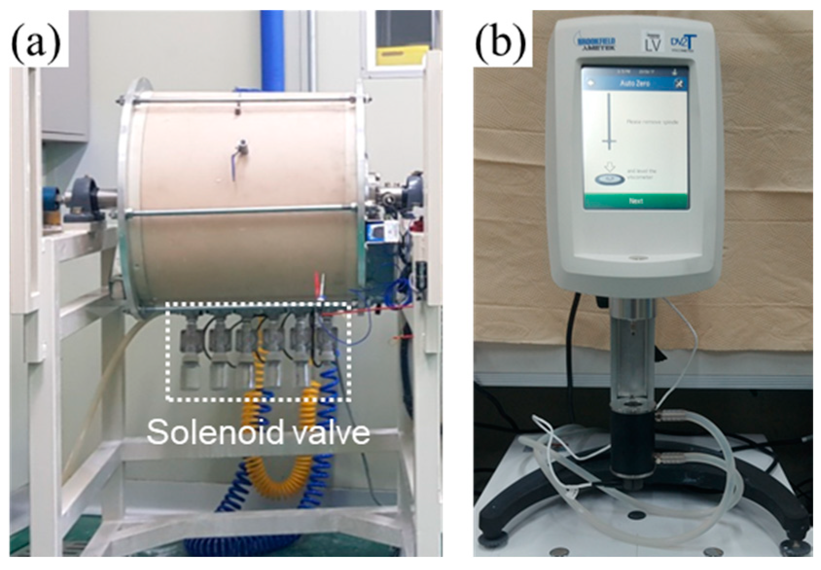
This section provides the description of the target process (i.e., ball mill) and the process dataset collected from it through CCD. Figure 1 shows a simplified schematic diagram for the target process. Ball mills are the most widely used equipment to grind ceramic powders to make their size appropriate, and to mix these powders with solvents and additives; after finishing ball milling, we obtain a slurry in which they are mixed together. To do this, after putting grinding media (e.g., balls), powders, solvents, and some additives into a closed cylindrical container (also called drum), in order, we rotate this container horizontally at a steady speed. While, the container rotates, the balls repeat climbing up its inner wall and then falling to the ground (i.e., they cascade); these behaviors enable us to evenly blend powders, solvents, and additives together. In addition, as powder particles move between the balls and between the balls and the inner wall, they are broken into smaller particles effectively. The quality of the slurry is usually evaluated, based on its viscosity and particle size distribution, before the slurry is fed into the next-stage unit process (i.e., spray dryer) to produce granules. In this study, we only focus on slurry viscosity that has significant impact on the efficiency of the spray dryer. Figure 2 shows the ball mill with an internal volume of 50 L and an internal diameter of 40 cm equipped for collecting the experiment dataset, and a rotating disk viscometer (DV2TLV) used to measure the values of slurry viscosity.
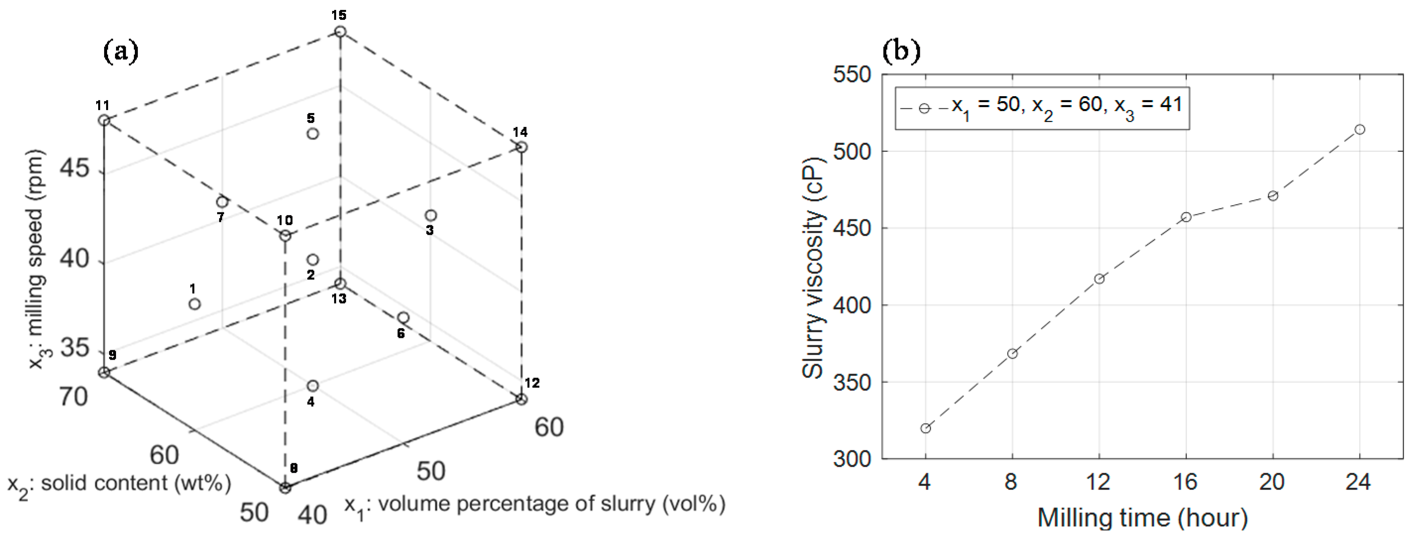
In this paper, volume percentage of slurry (vol%), solid content (wt%), milling speed (rpm), and milling time (h) are considered as key controllable factors for slurry viscosity. The volume percentage of slurry is the ratio of the volume of slurry to the volume of balls; the solid content equals the weight of powders divided by the weight of slurry; the milling speed and time are the rotation speed and the operation time of the ball mill, respectively. To gather input-output observations from the ball mill, ranges and levels for the three factors except for the milling time are set as tabulated in Table 1, and as shown in Figure 3a, fifteen experiments are designed; the range of each factor was determined by taking the opinions from field experts in ceramic industry. In every experiment, balls with the diameter of 10 mm were used, and the total weight and volume of these balls are 58.8 kg and 25 L, respectively. In each of the 15 experiments, together, the precise amounts of powders (i.e., Al2O3), solvent (i.e., ion-exchanged water), and additives (i.e., dispersant and binder) that fulfill the corresponding experimental conditions were supplied to the container, and it was operated for 24 h. During its operation, the values of slurry viscosity were measured every 4 h, and because of this, the milling time was excluded in the design of experiment. That is, the milling time is not included in the experimental design, but considered as a key controllable factor affecting the viscosity. Small amounts of samples were taken from the solenoid valves (see Figure 2a) installed in the bottom of the drum in 4-h intervals. Their values of viscosity were measured by the viscometer (see Figure 2b). Figure 3b shows the behavior of the measured viscosity values when the values of the three controllable factors are set as the center point in Figure 3a indicated by ‘2′; in this case, as can be seen from this figure, the slurry viscosity goes up steadily over time. Table 2 presents the experimental dataset collected from the target ball mill by conducting 15 experiments designed by CCD; these experiments were performed in random order. From the collected dataset, we can prepare 90 data points, each of which consists of 4 inputs and single output, to train the 2nd-order polynomial model.

5. Experimental Results and Discussion

In this section, to verify the performance, the proposed method summarized in Algorithm 1 is applied to the process dataset gathered from the target ball mill. Before describing the results of process modeling and optimization, let us look at scatter plots and main effect plots for the target dataset. Scatter plot is a visualization tool to intuitively check the relationships (e.g., positive or negative; linear or nonlinear) between input and output variables, here, the input-output coordinate points are displayed at two-dimensional planes. The main effect plot displaying level means and overall mean of a quality characteristic is effective for visualizing the effects of controllable factors on it based on a dataset collected by experimental design. Level means are the sample means of output variables calculated only from the observations whose jth input values are equal to a certain level; overall mean is the sample mean of output variable calculated from all observations.
Figure 4 shows the scatter plots between four input variables x1, ..., x4, and output variable y; here, reference lines indicated by black lines are the 2nd-order polynomial curves, least squares fitted to two-dimensional coordinate points. As shown in Figure 4a,b, y is negatively and positively correlated with x1 and x2, respectively. In Figure 4c, we can see the nonlinear relation between x3 and y, which can be captured by 2nd-order polynomials, but this is relatively weaker than those presented in Figure 4a,b. As Figure 4d indicates, there exists nonlinear and positive correlations between x4 and y; it is observed that as the milling time becomes longer, the increase of slurry viscosity is saturated.
Figure 5 presents the main effect plots for four controllable factors, and the ranges of level means (i.e., differences between maximum and minimum of level means) for them. In these main effect plots, level means are denoted by black circles and connected by black lines, and overall means are indicated by horizontal dashed black lines. In Figure 5e, the values of the ranges are described by a bar graph. It can be expected that if the level means are close to the overall mean, a controllable factor has no apparent effect on a quality characteristic. We can also expect that as the range values becomes larger, the effects of controllable factors on a quality characteristic becomes greater [30]. As can be seen visually from Figure 5c, the level means and overall mean relevant with x3 are extremely close in comparison with the other variables; in Figure 5a,b,d, the maximum and minimum of level means are far away from overall means compared with Figure 5c. As shown in Figure 5e, the range value relevant with x4 is the largest, and followed by those for x2 and x1; the range value of x3 is very small compared to those of others.
From now on, we present the results of applying the proposed CI-based process optimization method to the ball mill dataset and the discussion about the advantages of the proposed method. Before performing 2nd-order polynomial regression analysis, each input variable should be standardized to be bounded in the interval [−1, 1].

5.1. Results of Second-Order Polynomial Regression Analysis

In this paper, to formulate the functional relationship between the four controllable factors and the slurry viscosity of the target ball mill, we make use of the 2nd-order polynomial regression model presented in Equation (1). On the basis of the experiment dataset listed in Table 2, the model parameters can be estimated using the method of least squares; the total number of regression coefficients to be estimated is p’ = 1 + 2p + p(p − 1)/2 = 15 because the number of input variables is p = 4. Table 3 summarizes the results of estimating these coefficients; in this table, we list the estimates of coefficients, their standard errors (SEs), their t-statistics that equal to the values of estimates divided by their SEs, and the p-values of these t-statistics. The estimated coefficient β ^ 1 for x1 has the negative value, −80.80, since the volume percentage of slurry is negatively correlated with the slurry viscosity (see Figure 4a); on the contrary, the estimated coefficients for x2 and x4 are positive values, i.e., β ^ 2 = 105.08 and β ^ 4 = 105.01, respectively, because as the solid content or the milling time increase, the slurry viscosity also increases (see Figure 4b,d).
Determining whether it is possible to exclude a certain term from the full model with p’ coefficients can be determined based on the relevant p-value; the regression coefficients with large p-values have large variance, and thus, their precision is degraded. In general, the regression terms with the p-values larger than 0.05 or 0.01 are regarded to be statistically insignificant, so that we can drop these insignificant terms from the model. As tabulated in Table 3, the p-values of the regression coefficients β3, β12, β23, β11, and β22 are larger than 0.05. The coefficient β3 is not significant since y is not linear but weakly nonlinear in x3 (see Figure 4c). The p-values of the coefficients for x1 and x2 are very small, but the coefficients for their quadratic terms x 1 2 and x 2 2 have very large p-values; this tells us that y is affected by the input variables x1 and x2 not nonlinearly but linearly (see Figure 4a,b). Since the p-values of β12 and β23 are very large, it is obvious that the interaction terms x1x2 and x2x3 should be excluded from the full model, the remaining interaction terms with the p-values smaller than 0.05 should remain in the regression model.
After dropping the terms, x3, x1x2, x2x3, x 1 2 , and x 2 2 with the p-values of their coefficients larger than 0.05 from the full model, and then fitting the reduced model to the same dataset, we can obtain the following functional relationship:
y ^ ( x ) = 439.05 ( 12.99 ) 80.80 ( 7.61 ) x 1 + 105.08 ( 7.61 ) x 2 + 105.01 ( 9.10 ) x 4 19.32 ( 8.51 ) x 1 x 3 30.38 ( 11.14 ) x 1 x 4 + 21.31 ( 11.14 ) x 2 x 4 + 38.42 ( 11.14 ) x 3 x 4 + 29.97 ( 13.18 ) x 3 2 81.38 ( 15.57 ) x 4 2
where in the bottom of each estimated coefficient, its SE is also presented in parentheses; note that the values of coefficients and SEs in Equation (9) are slightly different from those in Table 3, since they are re-estimated without the terms, x3, x1x2, x2x3, x 1 2 , and x 2 2 . By modifying the full model in this way, the number of coefficients has been reduced from 15 to 10. In addition, the value of R2 has been reduced by 0.004 (from 0.865 to 0.861), but the value of adjusted R2 has increased by 0.006 (from 0.84 to 0.846). The R2 and adjusted R2 are the statistics used to determine how well the regression models are fitted to the target dataset; these values lie in the interval [0, 1], and as they get closer to 1, the goodness of fit of the regression model becomes better. It is well-known that the adjusted R2 is more suitable for preventing the model from overfitting than the R2 [5]; thus, it makes sense to exclude the insignificant terms from the full model because the adjusted R2 has increased. Moreover, the F statistic used to test the statistical significance of the regression model has increased by 20.8 (from 34.5 to 55.3); the larger the F statistic, the greater the statistical significance of these models. In summary, it is obvious that by removing the insignificant terms from the full model, we can obtain the more statistically significant and transparent model described in Equation (9).
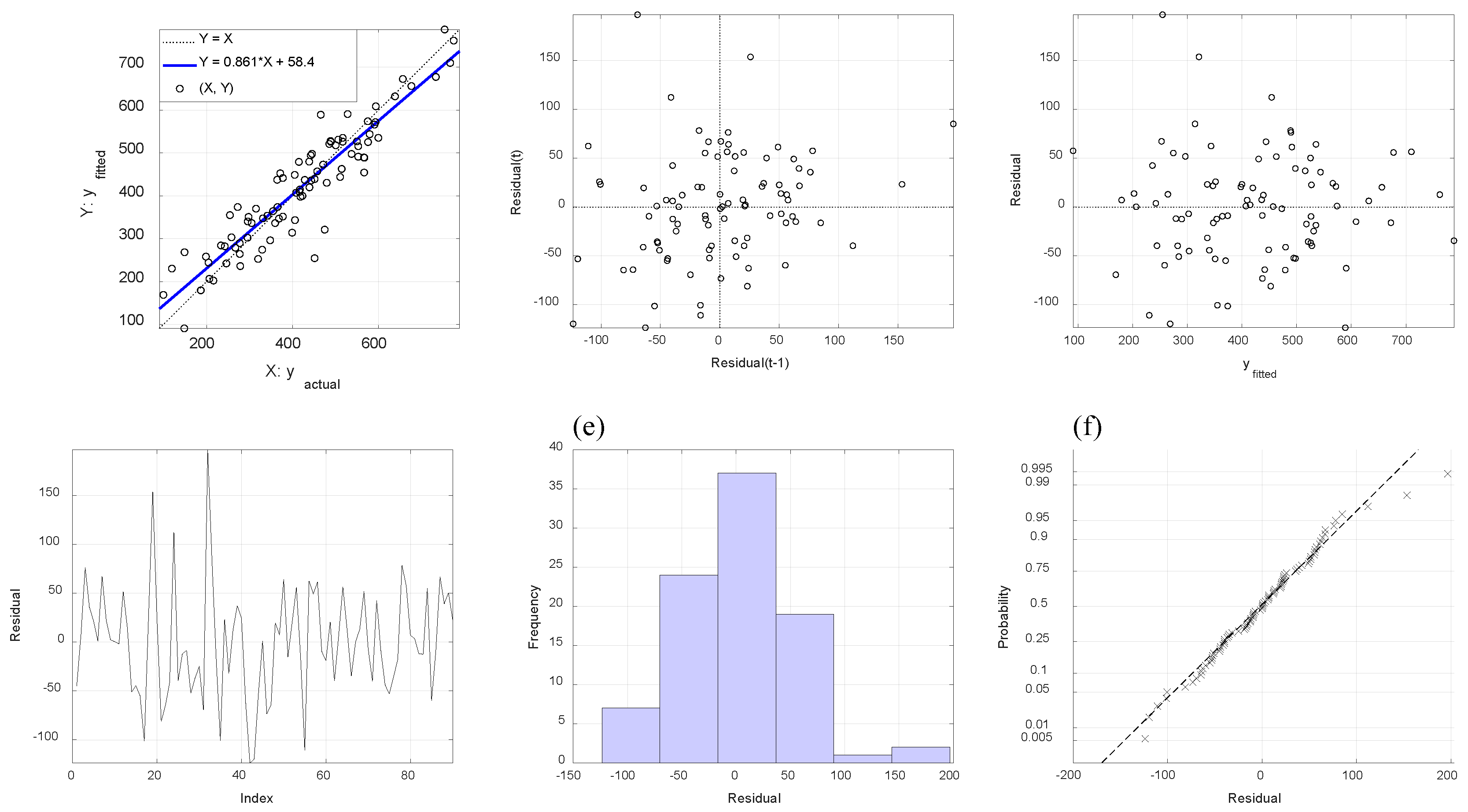
Next, to validate the resulting model in Equation (9), we present the scatter plot between actual outputs yi and predicted outputs y ^ i , and the results of analyzing the residuals r i = y i y ^ i , i = 1, ..., 90, one by one. Figure 6a shows the scatter plot between yi and y ^ i , and Figure 6b–f describe visualization tools to check the independence, homoscedasticity (i.e., constant variance), white noise properties, symmetry about zero, and normality of the error term ε in Equation (1). In Figure 6a, black circles correspond to coordinate points (yi, y ^ i ), i = 1, ..., 90, and dotted black and thick blue lines are the straight line X = Y and least squares fitted line to these points, respectively. Since there exists strong linear correlation between yi and y ^ i , it is apparent that the regression model describes the target process dataset adequately. Figure 6b is the scatter plot of the points (ri−1, ri), i = 2, ..., 90, to investigate the independence of ε; as can be seen from this figure, since there is no clear positive or negative correlation, the error term ε meets the independence assumption. Figure 6c shows the scatter plot between the fitted values y ^ i and the residuals ri to check the homoscedasticity of ε; it is observed that the residual values do not significantly increase or decrease with the fitted values. Figure 6d indicates the line plot of the residuals to confirm their white noise properties. In this figure, we can see that the sample mean of them is approximately equal to zero and they also show irregular behaviors; the characteristics of the residuals are roughly similar with those of white noise. Figure 6e,f describe the histogram and normal probability plots of the residuals, respectively; these figures indicate that the residuals do not depart from the symmetry and normality severely. To sum up, from Figure 6, we can conclude that the calculated residuals, ri, i = 1, ..., 90, based on Equation (9) do not violate the general assumptions for the error term ε considerably.
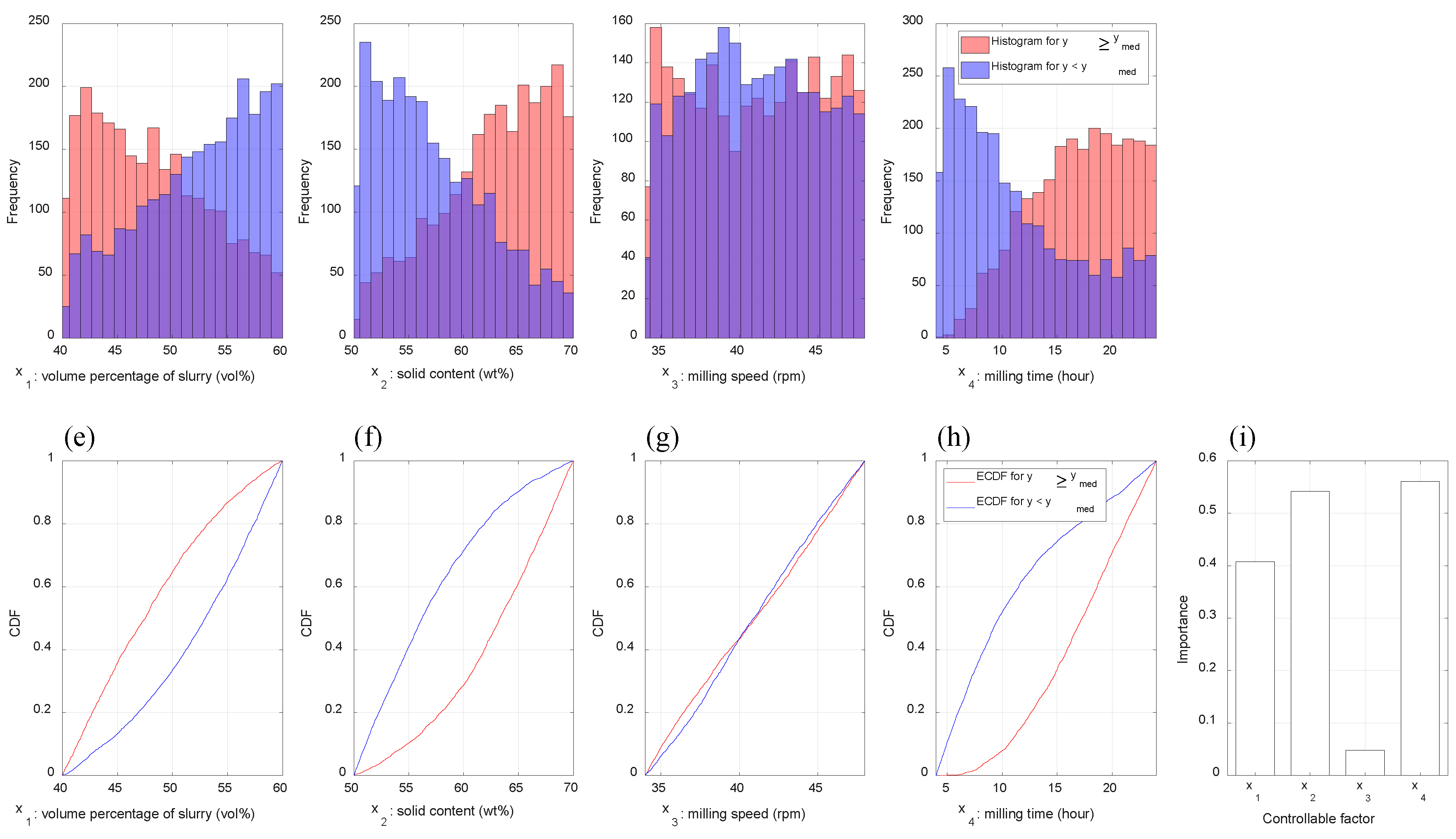
Now, let us look at the results of estimating the importance values of input variables using the MC-based method (see Section 2.2), presented in Figure 7. To do this, we generate N = 5000 random vectors x(i) 4 . Figure 7a–d show the histograms for each component of x(i) 4 , i = 1, ..., 5000; here, histograms related with those belonging to Xlarge and Xsmall are displayed as pink and shaded blue colors, respectively. Figure 7e–h depict empirical (red and blue) CDFs corresponding to each of the two histograms. In Figure 7a–h, for convenience of interpretation, the horizontal axis ranges have been recovered to their original ranges. Figure 7i is the bar graph for the estimated importance values of four controllable factors. As can be viewed from Figure 7a,b, as the values of x1 or x2 change, the frequencies increase or decrease nearly linearly; in Figure 7c,d, the frequencies change with the values of x3 and x4 nonlinearly. From Figure 7g, one can easily notice that the two CDFs of x3 are extremely similar to each other, thus, it is valid to say that the input x3 will have little impact on the output y. The input x4 has the greatest difference between the red and blue CDFs, and followed by x2 and x1. In other words, x4 has the highest estimated importance value, and followed by x2 and x1, and that of x3 is the lowest. Comparing Figure 5e and Figure 7i, we can see that these two bar graphs are slightly different; this may be due to the fact that the former based on main effect plots does not consider interaction effects between input variables, and the latter was obtained after dropping the insignificant terms, x3, x2x3, x 1 2 , and x 2 2 , from the full model.
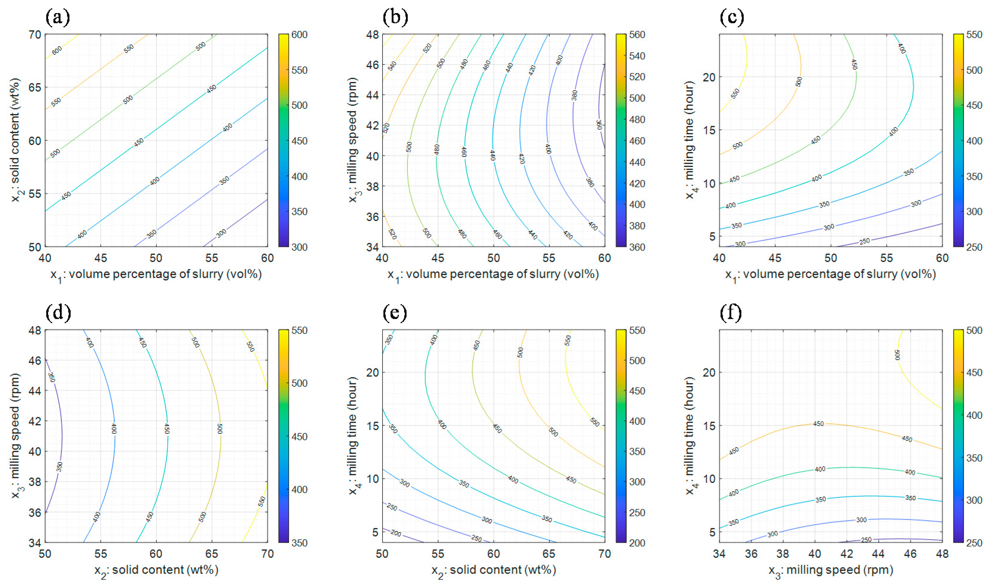
Next, let us take a look at the response surface and contour plots for Equation (9), described in Figure 8 and Figure 9, respectively. To obtain each plot, we first prepare grid coordinates based on X-axis and Y-axis variables. Then, by plugging these coordinates into Equation (9), we calculate its output values. In doing this, their median values are substituted into Equation (9), in the case of those inputs not included in the coordinates. In common with Figure 7, the ranges of X- and Y-axes have returned to their original ranges. By examining the response surface and contour plots closely, we can see how the pairs of axes variables interact and then affect the output variable y visually. As shown in Figure 8a and Figure 9a, as the value of x1 increases or that of x2 decreases, the value of y decreases; this was also confirmed in the scatter plots in Figure 4a,b. That is, these two variables linearly influence on y, and x2 has a greater effect on y than x1. In Figure 8b and Figure 9b, as the value of x1 becomes larger, the value of y becomes smaller. Also, as the value of x3 increases, the value of y decreases and then increases. Since the value of y changes more when the value of x1 is changed than when that of x3 is changed, it is valid to say that x1 is the more important controllable factor than x3. From Figure 8c and Figure 9c, one can easily notice that the value of y changes much more when the value of x4 increases than when the value of x1 increases. There exists clear nonlinear relationship between y and x4, and the increase of the value of x4 tends to dampen the increase of the value of y. When the value of x4 is small (i.e., in the early stage of milling operation), x4 influences much more on y than x1; as the milling time passes, the effect of x1 on y becomes larger than that of x4. Figure 8d and Figure 9d indicate that x2 has a much greater impact on y than x3; in these figures, the shapes of contours indicated by different colors are very similar to each other because the interaction term x2x3 was removed from the full model. Figure 8e and Figure 9e tell us that as the value of x4 becomes larger, this slows down the increase of the value of y; here, we can also confirm that as the value of x4 increases, the influence of x2 on y gets larger. In Figure 8f and Figure 9f, we can see that x4 influences much more on y than x3, and as the value of x4 becomes larger, the value of y is saturated.

5.2. Results of Confidence Interval-Based Process Optimization

In this subsection, we describe the results of applying the PSO algorithm to the objective function F(x) = | y target y ^ ( x ) | defined based on Equation (9). The values of α, L, and L’ in Algorithm 1 are set as 0.05, 100, and 10, respectively, and Table 4 lists the user-defined parameters used in the PSO algorithm.
First, let us take a look at the results of finding the values of controllable factors achieving the slurry viscosity of 550 cP (i.e., ytarget = 550); as can be seen from Figure 9, it is obvious that there exists an infinite number of solutions for this process optimization problem. Table 5 lists L’ = 10 solutions found by the proposed method, CIs enclosing their outputs of Equation (9), and their lengths. Among these solutions, the most statistically significant solution is x ( 1 ) * = [47.07, 63.93, 45.59, 16.29]T. Figure 10 shows the trajectories of each component in xgbest, and the trajectory of y ^ ( x g b e s t ) during the search for the x ( 1 ) * using the PSO algorithm; similar to Figure 8, the Y-axis ranges have been recovered to their original ranges. In the initiation stage for the search, there are some fluctuations in these trajectories; as the updates are repeated and then the number of iterations become larger than about 120, xgbest and y ^ ( x g b e s t ) have converged to x ( 1 ) * and 550, respectively. Figure 11 shows the contour plots where the solution x ( 1 ) * is indicated by red asterisks; as described in this figure, x ( 1 ) * is located at the coordinate points whose height values are exactly equal to the target value ytarget = 550. Based on Table 5, one can easily notice that the lengths of CIs for the 10 solutions are slightly different from each other; however, the values of controllable factors vary from solution to solution considerably. It is worthwhile to emphasize that although x ( 1 ) * is the best solution from a statistical viewpoint, this may not always fulfill the requirements for the users. The proposed method recommends several statistically significant solutions so that among them the users can flexibly choose and use the suitable solutions for process conditions. For example, if the users want the milling time to be shorter than 16.29 h in x ( 1 ) * and, at the same time, want the slurry viscosity to be equal to the target value, i.e., ytarget = 550, they can set the values of controllable factors on the basis of x ( 8 ) * instead of x ( 1 ) * ; in this case, the milling time can be reduced by about 2 h, the value of the volume percentage of slurry and solid content become higher by 0.9 vol% and 0.36 wt%, respectively, and the milling speed becomes faster than before. The difference in the lengths of CIs between x ( 1 ) * and x ( 8 ) * is 3.9, and it is negligible. If it is desirable to decrease the value of solid content to be smaller than 63.93 wt% in x ( 1 ) * , the 6th solution x ( 6 ) * can be used instead; in this case, the milling time increases by 0.77 h, the value of the volume percentage of slurry decreases by 2.77 vol%, and the milling speed is similar to each other; the difference in the lengths of CIs between x ( 1 ) * and x ( 6 ) * is 3.9, and it is also negligible.
Table 6 and Table 7 summarize the results of applying the proposed method to obtain the values of controllable factors achieving the slurry viscosities of 500 cP and 450 cP, respectively; in these two tables, the differences in the lengths between the first and last solutions are 3.21, and 3.16 (typically negligible), respectively. This means that the statistical significances of the solutions in each table are similar with each other, and thus, the users can select and use the most appropriate solutions for field situations among them. If the users want to operate the target ball mill for a relatively short period of time and, at the same time, want to obtain the slurry with the viscosity value of 500 cP, they are able to utilize the 6th solution x ( 6 ) * in Table 6; if it is desirable for the solid content to be relatively low, the 5th solution x ( 5 ) * in Table 6 can be used to set the values of process parameters. When the target value for slurry viscosity is equal to ytarget = 450, the users can choose the proper solutions satisfied with their requirements from the recommended solutions listed in Table 7.

5.3. Discussion

In this subsection, we shall summarize the strengths of the proposed CI-based process optimization method. The main strengths include that when a unique solution for process optimization problems does not exist, and thus, different solutions can be found whenever optimization algorithms are executed, the proposed method can assess the qualities of these different solutions from a statistical point of view. Recall that, as described in Figure 11, there is an infinite number of different solutions achieving the same quality characteristic as a desired target value ytarget. In the proposed method, the qualities of them are evaluated on the basis of the CI in Equation (2); it is important to remark that as the lengths of their CIs become shorter, their uncertainties caused by such things as measurement errors and/or uncontrollable factors decrease. The second strength is that since the proposed method recommends the L’ statistically significant solutions for the users (see Table 5, Table 6 and Table 7), it can provide them with a variety of choices. As explained in Section 5.2, it is undesirable to recommend only the first solution x ( 1 ) * for the users because it may not fulfill the requirements for them. The proposed method enables the users to flexibly select and use the solutions suitable for practical situations among the L’ solutions.
Prior to completing this subsection, let us describe how the importance values of controllable factors presented in Figure 5e and Figure 7i can help the process operators and engineers. First, these important values provide guidance on which controllable factors should be set more correctly so as to optimize quality characteristics; it is entirely fair to say that the controllable factors with larger importance values should be more precisely set to the values of the preferred solution. For example, in the case of the target ball mill, the milling time should be set most accurately because it has the biggest importance value; the milling speed with the smallest importance value may be loosely set. Second, the importance values can serve as a good reference for performing additional experimental designs. For example, unimportant factors may be excluded from these additional experimental designs, and thus one can only focus on important factors when planning them. In addition, one can increase the number of levels for important factors to closely examine their effects on quality characteristics while reducing the number of levels for unimportant factors.

6. Conclusions

In this paper, we proposed a CI-based process optimization method using second-order polynomial regression analysis. Recall that if the goal of process optimization is to make the quality characteristics equal to the user-defined target values, we cannot obtain a unique solution; in this case, whenever optimization algorithms are executed, different solutions can be obtained. In this paper, after obtaining several different solutions by applying the PSO algorithm repeatedly, the qualities of these solutions are evaluated on the basis of the CIs (see Equation (2)); the solutions are sorted in ascending order according to the lengths of their CIs, and then the first few solutions are recommended for the users. To verify the performance, the proposed method was applied to the process dataset collected from the target ball mill; here, the aim of the proposed method is to obtain the values of the controllable factors achieving the target values of slurry viscosity. The simulation results showed that the proposed method can provide several statistically significant solutions; among these solutions, the users can flexibly select and use the proper solutions for practical situations.
In future research, we will consider improving the proposed method to be applicable even when machine learning techniques [31] are used to formulate the input-output relations. In this case, the number of collected input-output observations should be large enough to prevent the overfitting problem. The regression surfaces based on machine learning techniques are, in general, more uneven than those based on the second-order polynomial regression analysis; therefore, instead of PSO algorithm, more advanced optimization algorithms presented in [22,23,24,25] should be applied.

Author Contributions

Conceptualization, J.Y., H.J. and S.K.; methodology, J.Y. and H.J.; software, J.Y.; validation, S.Y., J.K. and Y.L.; formal analysis, J.Y.; investigation, J.Y. and H.J.; resources, K.-T.L. and S.-S.R.; data curation, S.K., S.-S.R. and H.J.; writing—original draft preparation, J.Y.; writing—review and editing, H.J., S.Y. and J.K.; visualization, J.Y.; supervision, K.-T.L. and S.-S.R.; project administration, Y.L., K.-T.L. and S.-S.R.; funding acquisition, Y.L. and K.-T.L. All authors have read and agreed to the published version of the manuscript.

Funding

This work was supported by the Ministry of Trade, Industry and Energy (MOTIE), South Korea, through the i-Ceramic platform construction project-i-Ceramic manufacturing innovation platform (Development of Cloud Big Data Platform for the Innovative Manufacturing in Ceramic Industry) under Grant 20004367.

Conflicts of Interest

The authors declare no conflict of interest.

References

  1. Rao, R.V. Advanced Modeling and Optimization of Manufacturing Processes: International Research and Development; Springer Science & Business Media: Berlin/Heidelberg, Germany, 2010. [Google Scholar] [CrossRef]
  2. Castillo, E.D. Process Optimization: A Statistical Approach; Springer Science & Business Media: Berlin/Heidelberg, Germany, 2007. [Google Scholar] [CrossRef]
  3. Dejaegher, B.; Heyden, Y.V. Experimental designs and their recent advances in set-up, data interpretation, and analytical applications. J. Pharm. Biomed. Anal. 2011, 56, 141–158. [Google Scholar] [CrossRef] [PubMed]
  4. Draper, N.R.; Smith, H. Applied Regression Analysis; John Wiley & Sons: Hoboken, NJ, USA, 1998. [Google Scholar] [CrossRef]
  5. Hastie, T.; Tibshirani, R.; Friedman, J. The elements of Statistical Learning: Data Mining, Inference, and Prediction; Springer Science & Business Media: Berlin/Heidelberg, Germany, 2009. [Google Scholar] [CrossRef]
  6. Ebadnejad, A.; Karimi, G.R.; Dehghani, H. Application of response surface methodology for modeling of ball mills in copper sulphide ore grinding. Powder Technol. 2013, 245, 292–296. [Google Scholar] [CrossRef]
  7. Parida, M.K.; Joardar, H.; Fout, A.K.; Routaray, I.; Mishra, B.P. Multiple response optimizations to improve performance and reduce emissions of Argemone Mexicana biodiesel-diesel blends in a VCR engine. Appl. Thermal Eng. 2019, 148, 1454–1466. [Google Scholar] [CrossRef]
  8. Adesina, O.A.; Abdulkareem, F.; Yusuff, A.S.; Lala, M.; Okewale, A. Response surface methodology approach to optimization of process parameter for coagulation process of surface water using Moringa oleifera seed. S. Afr. J. Chem. Eng. 2019, 28, 46–51. [Google Scholar] [CrossRef]
  9. Costa, N.; Garcia, J. Using a multiple response optimization approach to optimize the coefficient of performance. Appl. Thermal Eng. 2016, 96, 137–143. [Google Scholar] [CrossRef]
  10. Chen, Z.; Shi, Y.; Lin, X.; Yu, T.; Zhao, P.; Kang, C.; He, X.; Li, H. Analysis and optimization of process parameter intervals for surface quality in polishing Ti-6Al-4V blisk blade. Results Phys. 2019, 12, 870–877. [Google Scholar] [CrossRef]
  11. Li, Y.X.; Xu, Q.Y.; Guo, R.T.; Wang, Z.Y.; Liu, X.Y.; Shi, X.; Qiu, Z.Z.; Qin, H.; Jia, P.Y.; Qin, Y.; et al. Removal of NO by using sodium persulfate/limestone slurry: Modeling by response surface methodology. Fuel 2019, 254. [Google Scholar] [CrossRef]
  12. Aggarwal, A.; Singh, H.; Kumar, P.; Singh, M. Optimizing power consumption for CNC turned parts using response surface methodology and Taguchi’s technique-a comparative analysis. J. Mater. Process. Technol. 2008, 200, 373–384. [Google Scholar] [CrossRef]
  13. Mohanty, S.; Mishra, A.; Nanda, B.K.; Routara, B.C. Multi-objective parametric optimization of nano powder mixed electrical discharge machining of AlSiCp using response surface methodology and particle swarm optimization. Alexandria Eng. J. 2018, 57, 609–619. [Google Scholar] [CrossRef]
  14. Zhang, C.; Chen, Z.; Mei, Q.; Duan, J. Application of particle swarm optimization combined with response surface methodology to transverse flux permanent magnet motor optimization. IEEE Trans. Magn. 2017, 53, 1–7. [Google Scholar] [CrossRef]
  15. Hasanien, H.M. Particle swarm design optimization of transverse flux linear motor for weight reduction and improvement of thrust force. IEEE Trans. Ind. Electron. 2010, 58, 4048–4056. [Google Scholar] [CrossRef]
  16. Nocedal, J.; Wright, S.J. Numerical Optimization; Springer Science & Business Media: Berlin/Heidelberg, Germany, 2006. [Google Scholar] [CrossRef] [Green Version]
  17. Talbi, E.G. Metaheuristics: From Design to Implementation; John Wiley & Sons: Hoboken, NJ, USA, 2009. [Google Scholar] [CrossRef]
  18. Richerson, D.W.; Lee, W.E. Modern Ceramic Engineering Properties, Processing, and Use in Design; CRC Press: Boca Raton, FL, USA, 2018. [Google Scholar] [CrossRef]
  19. Deng, B.; Shi, Y.; Yu, T.; Kang, C.; Zhao, P. Multi-response parameter interval sensitivity and optimization for the composite tape winding process. Materials 2018, 11, 220. [Google Scholar] [CrossRef] [PubMed] [Green Version]
  20. Yin, X.; He, Z.; Niu, Z.; Li, Z.S. A hybrid intelligent optimization approach to improving quality for serial multistage and multi-response coal preparation production systems. J. Manuf. Syst. 2018, 47, 199–216. [Google Scholar] [CrossRef]
  21. Bera, S.; Mukherjee, I. A multistage and multiple response optimization approach for serial manufacturing system. Eur. J. Oper. Res. 2016, 248, 444–452. [Google Scholar] [CrossRef]
  22. Precup, R.E.; David, R.C. Nature-inspired Optimization Algorithms for Fuzzy Controlled Servo Systems; Butterworth-Heinemann: Oxford, UK, 2019. [Google Scholar] [CrossRef]
  23. Wang, G.; Guo, L. A novel hybrid bat algorithm with harmony search for global numerical optimization. J. Appl. Math. 2013. [Google Scholar] [CrossRef]
  24. Haber, R.E.; Beruvides, G.; Quiza, R.; Hernandez, A. A simple multi-objective optimization based on the cross-entropy method. IEEE Access 2017, 5, 22272–22281. [Google Scholar] [CrossRef]
  25. Tharwat, A.; Hassanien, A.E. Quantum-behaved particle swarm optimization for parameter optimization of support vector machine. J. Classif. 2019, 36, 576–598. [Google Scholar] [CrossRef]
  26. Engelbrecht, A.P. Computational Intelligence: An Introduction; John Wiley & Sons: Hoboken, NJ, USA, 2007. [Google Scholar] [CrossRef]
  27. Kennedy, J.; Eberhart, R. Particle swarm optimization. In Proceedings of ICNN’95-International Conference on Neural Networks; IEEE: Piscataway, NJ, USA, 1995; Volume 4, pp. 1942–1948. [Google Scholar] [CrossRef]
  28. Ratnaweera, A.; Halgamuge, S.K.; Watson, H.C. Self-organizing hierarchical particle swarm optimizer with time-varying acceleration coefficients. IEEE Trans. Evol. Comput. 2004, 8, 240–255. [Google Scholar] [CrossRef]
  29. Del Valle, Y.; Venayagamoorthy, G.K.; Mohagheghi, S.; Hernandez, J.C.; Harley, R.G. Particle swarm optimization: Basic concepts, variants and applications in power systems. IEEE Trans. Evol. Comput. 2008, 12, 171–195. [Google Scholar] [CrossRef]
  30. Kwak, J.S. Application of Taguchi and response surface methodologies for geometric error in surface grinding process. Int. J. Mach. Tools Manuf. 2005, 45, 327–334. [Google Scholar] [CrossRef]
  31. Castaño, F.; Beruvides, G.; Villalonga, A.; Haber, R.E. Self-tuning method for increased obstacle detection reliability based on internet of things LiDAR sensor models. Sensors 2018, 18, 1508. [Google Scholar] [CrossRef] [PubMed] [Green Version]
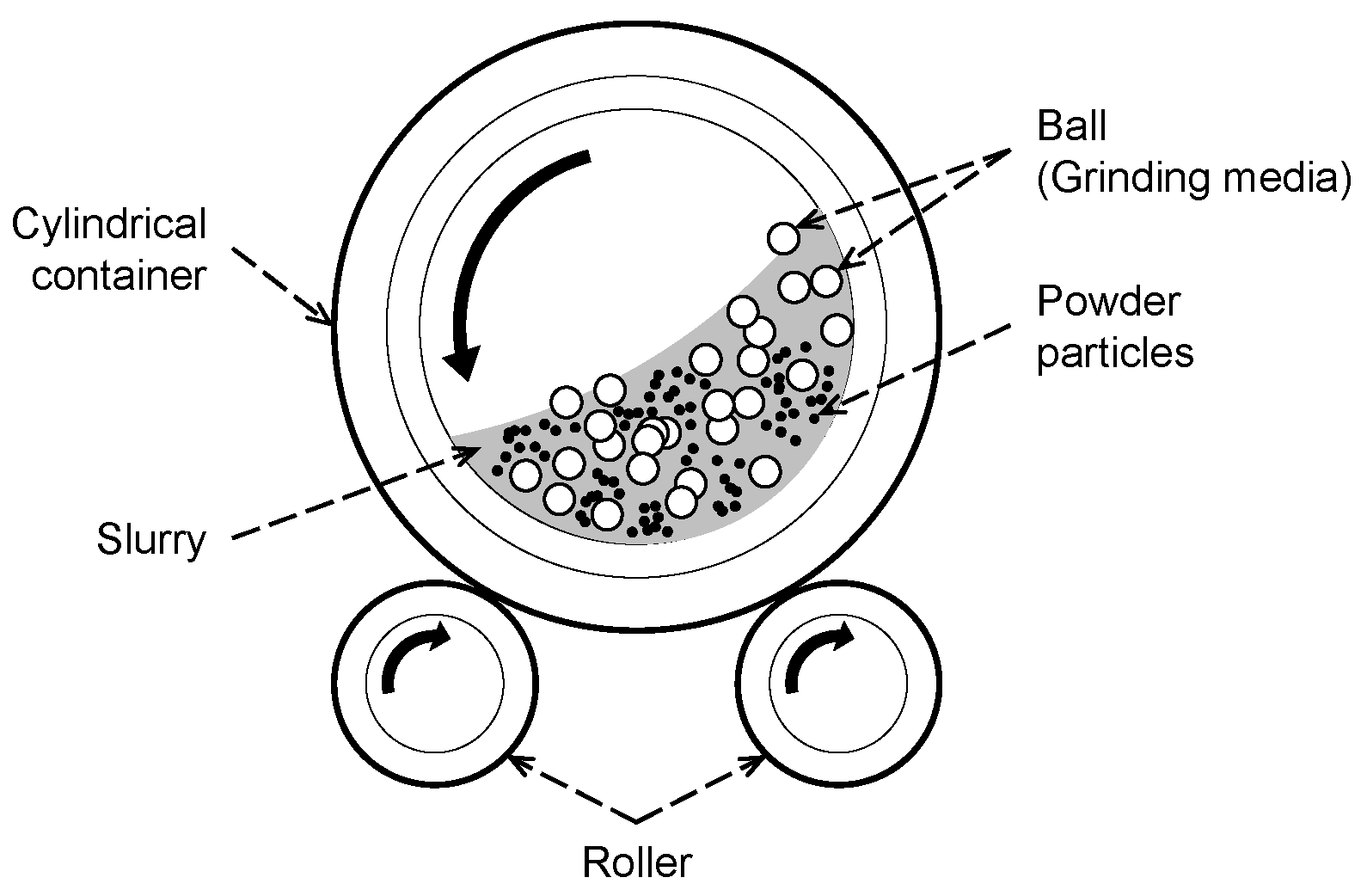
Figure 1. Simplified schematic diagram for the target ball mill. Adapted from FIGURE 12.11 in [18], with the permission of ASM International.
Processes 08 01206 g001
Figure 2. Target ball mill equipped for collecting experiment dataset and viscometer used to measure slurry viscosity: (a) Ball mill with the internal volume of 50 L and the interval diameter of 40 cm; (b) rotating disk viscometer (DV2TLV).
Processes 08 01206 g002
Figure 3. (a) Arrangement of 15 tests designed by CCD; (b) measured values of slurry viscosity at the center point.
Processes 08 01206 g003
Figure 4. Scatter plots between input and output variables: (a) x1 vs. y; (b) x2 vs. y; (c) x3 vs. y; (d) x4 vs. y.
Processes 08 01206 g004
Figure 5. (a) main effect plot for x1; (b) main effect plot for x2; (c) main effect plot for x3; (d) main effect plot for x4; (e) ranges of level means for x1, ..., x4.
Processes 08 01206 g005
Figure 6. (a) scatter plot between yi and y ^ i ; (b) scatter plot between ri−1 and ri; (c) scatter plot between y ^ i and ri; (d) line plot for ri; (e) histogram for ri; (f) normal probability plot for ri.
Processes 08 01206 g006
Figure 7. Results of estimating the importance values of controllable factors using the MC-based method: (a) histograms for x1; (b) histograms for x2; (c) histograms for x3; (d) histograms for x4; (e) ECDFs for x1; (f) ECDFs for x2; (g) ECDFs for x3; (h) ECDFs for x4; (i) estimated importance values of four controllable factors.
Processes 08 01206 g007
Figure 8. Response surface plots for Equation (9): (a) (x1, x2, y); (b) (x1, x3, y); (c) (x1, x4, y); (d) (x2, x3, y); (e) (x2, x4, y); (f) (x3, x4, y).
Processes 08 01206 g008
Figure 9. Contour plots for Equation (9): (a) (x1, x2); (b) (x1, x3); (c) (x1, x4); (d) (x2, x3); (e) (x2, x4); (f) (x3, x4).
Processes 08 01206 g009
Figure 10. Trajectories of xgbest and y ^ ( x g b e s t ) during the search for the x ( 1 ) * using the PSO algorithm: (a) trajectory of x 1 g b e s t ; (b) trajectory of x 2 g b e s t ; (c) trajectory of x 3 g b e s t ; (d) trajectory of x 4 g b e s t ; (e) trajectory of y ^ ( x g b e s t ) .
Processes 08 01206 g010
Figure 11. Contour plots with the solution x ( 1 ) * achieving y ^ ( x ( 1 ) * ) = 550: (a) (x1, x2); (b) (x1, x4); (c) (x2, x4).
Processes 08 01206 g011
Table 1. Ranges and levels for the three controllable factors.
Controllable FactorLevel
−101
x1: slurry volume (vol%)405060
x2: solid content (wt%)506070
x3: milling speed (rpm)344148
Table 2. Experiment dataset collected from the target ball mill by conducting 15 tests designed by CCD.
Test IDx1x2x3Slurry Viscosity (cP)
After 4 hAfter 8 hAfter 12 hAfter 16 hAfter 20 hAfter 24 h
Test 1406041258.0416.4565.8579.3592.8574.8
Test 2506041319.8368.4417.0457.2471.0514.2
Test 3606041216.0233.4295.8315.0272.4377.4
Test 4506034474.6423.0371.4414.6438.6566.4
Test 5506048204.6341.4428.4442.2489.0506.4
Test 650504199.6451.2399.0331.2254.4359.4
Test 7507041304.8451.2552.6590.4528.0465.6
Test 8405034148.8297.6408.0364.2377.4439.2
Test 9407034443.3599.4593.6676.2733.0656.4
Test 10405048119.4405.6479.4552.6516.6516.6
Test 11407048418.2488.2638.2766.4774.6753.4
Test 12605034206.4277.2348.0295.2242.4278.4
Test 13607034364.8405.0445.2485.4500.4567.0
Test 14605048148.2186.6246.0267.0277.2329.4
Test 15607048198.6354.6510.6537.0575.4549.6
Table 3. Results of estimating 15 regression coefficients using the method of least squares.
CoefficientEstimateStandard Errort-Statisticp-Value
β0439.00 15.10 29.08 0.0000
β1−80.80 7.75 −10.43 0.0000
β2105.08 7.75 13.57 0.0000
β33.01 7.75 0.39 0.6989
β4105.01 9.26 11.34 0.0000
β12−10.91 8.66 −1.26 0.2115
β13−19.32 8.66 −2.23 0.0286
β14−30.38 11.34 −2.68 0.0091
β23−5.55 8.66 −0.64 0.5233
β2421.31 11.34 1.88 0.0640
β3438.42 11.34 3.39 0.0011
β11−3.70 15.27 −0.24 0.8091
β223.82 15.27 0.25 0.8031
β3329.92 15.27 1.96 0.0538
β44−81.38 15.84 −5.14 0.0000
Table 4. User-defined parameters in the PSO algorithm.
nstmaxw(0)w(tmax)c1minc1maxc2minc2max
202000.90.40.52.50.52.5
Table 5. (ytarget = 550) Results of finding L’ = 10 solutions using the proposed method.
Orderx1x2x3x4CILength
147.0763.9345.5916.29[528.63, 571.37]42.73
246.4161.8044.6619.29[527.83, 572.17]44.34
350.5366.9134.8317.13[527.74, 572.26]44.52
448.3865.2335.0719.36[527.70, 572.30]44.60
550.0062.6048.0018.94[527.63, 572.37]44.75
644.3060.7145.5217.06[527.44, 572.56]45.12
749.9266.3834.1616.40[527.16, 572.84]45.67
846.1763.5748.0014.32[526.69, 573.31]46.63
948.1065.2135.5920.29[526.68, 573.32]46.64
1047.7565.2837.3719.10[526.67, 573.33]46.65
Table 6. (ytarget = 500) Results of finding L’ = 10 solutions using the proposed method.
Orderx1x2x3x4CILength
149.1361.6234.5416.27[480.23, 519.77]39.54
247.5261.5635.0014.87[480.08, 519.92]39.83
348.6561.6934.5315.38[480.01, 519.99]39.98
451.1561.6144.9519.51[479.39, 520.61]41.22
547.5759.9245.1016.56[479.18, 520.82]41.64
649.0265.4334.9611.66[479.07, 520.93]41.86
751.3465.1846.1814.20[479.02, 520.98]41.97
851.9561.8747.8016.75[478.97, 521.03]42.06
949.3261.0934.0017.95[478.64, 521.36]42.72
1048.5661.5637.4219.87[478.63, 521.37]42.75
Table 7. (ytarget = 450) Results of finding L’ = 10 solutions using the proposed method.
Orderx1x2x3x4CILength
148.4657.5835.0314.71[430.31, 469.69]39.38
250.3262.9436.2511.07[430.17, 469.83]39.65
352.6860.3146.1515.49[430.12, 469.88]39.77
453.6460.3435.5018.25[429.68, 470.32]40.64
548.2561.6736.8111.37[429.42, 470.58]41.16
647.1156.0646.6614.36[429.20, 470.80]41.60
749.0257.4645.1615.60[429.05, 470.95]41.89
846.6359.8445.3612.04[428.94, 471.06]42.12
950.2160.3537.0413.90[428.90, 471.10]42.20
1048.3762.1847.8810.79[428.73, 471.27]42.54