Article

Optimal-Setpoint-Based Control Strategy of a Wastewater Treatment Process

1
Department of Automation and Electrical Engineering, Dunarea de Jos University of Galati, Domneasca No. 47, 800008 Galati, Romania
2
Optimar SA Galati, Drum de Centura No. 3, 800248 Galati, Romania
*
Author to whom correspondence should be addressed.
Processes 2020, 8(10), 1203; https://doi.org/10.3390/pr8101203
Submission received: 25 August 2020 / Revised: 18 September 2020 / Accepted: 20 September 2020 / Published: 23 September 2020
(This article belongs to the Special Issue Control and Optimization of Wastewater Treatment Technology)

Abstract

:
This paper presents an optimal-setpoint-based control strategy of a wastewater treatment process (WWTP). The treatment plant serves the city of Galati, located in Eastern Romania, a city with a population of 250,000 inhabitants. As the treatment plant includes several control loops (based upon PI controllers), an efficient operation means the establishing of an optimal operating point regardless of the pluviometric regime (DRY, RAIN and STORM) or transitions between regimes. This optimal operating point is given by the optimal setpoint set (setpoints of the dissolved oxygen concentration in the aerated tanks, setpoint of the nitrate concentration, external recirculation flow, sludge flow extracted from the primary clarifier and excess sludge flow from the secondary clarifier) of the treatment plant control loops. The control algorithm has two distinct parts: the first part consists of computing the optimal aforementioned setpoints, based on the mathematical model of the treatment plant developed in SIMBA. For optimization (performed with genetic algorithms) an aggregate performance criterion that takes into consideration the quality of the effluent, the cost of the wastewater treatment as well as the percentage exceeding of the main parameters of the treated water was used; the second part consists of computing the optimal setpoint set which will be further applied directly in the process based on the membership to the current operating regime. The computation of the membership degrees to the current operating regime was performed with a fuzzification block, based on the information about the inflow rate in the biological treatment plant. For simulations, three data files of the influent were created, aiming at determining the optimal setpoints in each operating regime, and a fourth one containing an influent scenario able to globally test the system operation. The obtained results showed the efficiency of the biological treatment, the effluent quality index being about ten times lower than that of the influent. Furthermore, the genetic algorithm used in optimization determines accurately enough the minimum value of the performance criterion in the case of each pluviometric regime, the lowest value of the performance criterion being obtained in DRY operating regime and the highest values in RAIN and STORM regimes. This is mainly due to the increase of the treatment cost and to small exceeding of the limits of several quality parameters such as chemical oxygen demand and ammonium concentration in the two regimes mentioned above. The fuzzification block aims to achieve a smooth transition from one operating regime to another, thus determining easier operating regimes of the treatment plant actuators and contributing to the increase of their life cycle.

1. Introduction

Environmental protection is a priority of the economic and social development that aims at obtaining a clean and healthy environment that does not affect the development possibilities of future generations. It is, therefore, imperative to ensure the protection of the environment and the conservation of natural resources, especially water, according to the requirements of the sustainable economic and social development. Deterioration of the environment involves alteration of the physico-chemical and structural characteristics of the natural components of the environment, reduction of diversity or biological productivity of natural ecosystems, damage of the natural environment with effects on the quality of life, mainly caused by water, atmosphere and soil pollution, over-exploitation of the resources and their poor management and valorization.
The water is an essential natural resource for today’s society. Therefore, one of the great problems facing humanity is the provision of water resources for urban and rural communities, for various industrial and/or agricultural activities, given that the world’s population is constantly growing, and the industry is constantly evolving. In these conditions, this intensive use of water inevitably leads to its pollution, and by discharging polluted water into groundwater or surface water, to environmental pollution. In this regard, the issue of environmental protection and water resources management has become very pressing and in the permanent attention of the European Union (EU). The European Commission (EC) developed numerous directives [1,2] that show the concern of this European forum to prevent the degradation of the environment and the quality of water resources. This set of normative acts has materialized in a program for the protection of Europe’s water resources. A number of quality standards have been imposed with clear objectives for the protection of human health and the environment, including surface water, domestic water, fishery, shellfish (waters for growing various species of mollusks), groundwater and drinking water. One of these legislative directives imposed certain standards relating to the discharge of substances into surface waters. Other directives refer to the urban wastewater treatment (UWWT), to the prevention of pollution in the industrial and agricultural environment, to the water management in the natural hydrographic basins, etc.
Given the importance of the wastewater treatment field, research in this field has evolved in two directions:
  • modernization of wastewater collecting and treatment infrastructure in urban areas in parallel with the development of new wastewater treatment technologies;
  • development and use of new automation methods (mathematical modeling [3,4], control and state and parameter estimation [5,6,7,8]) in order to increase the efficiency of the wastewater treatment processes.
Thus, it can be stated that the wastewater treatment field has become an area addressed by numerous interdisciplinary research teams consisting of specialists in microbiology and biochemistry and last but not least, in automation and computer science. Given that these processes are nonlinear, very complex and strongly affected by uncertainties (parameter and model uncertainties), these processes have become a real challenge for specialists in modeling, identification and control in order to develop advanced methods for increasing the efficiency of the wastewater treatment processes.
Among the most well-known mathematical models reported by the literature and accepted by the international scientific community can be mentioned ASM models (Activated Sludge Models). These were developed within International Association on Water Quality (IAWQ), which became later International Water Association (IWA), by a working group led by Prof. Henze, which aimed at developing and applying mathematical models of biological treatment processes in the design and operation of treatment plants. The first activated sludge treatment model (ASM1) [9] describes the biological oxidation of carbon, the nitrification and denitrification and is, therefore, used to model the removal of carbon and nitrogen in the activated sludge treatment systems. It considers four processes: (1) the growth of autotrophic and heterotrophic bacteria, (2) their degradation, (3) the hydrolysis of the organic particles and (4) ammonification of soluble organic nitrogen. The reaction rate of each process is expressed as a series of Monod-type smooth switching functions, corresponding to certain conditions (for example aerobic, anoxic, anaerobic processes). The ASM2 model [10] is an extension of ASM1 and includes the biological and chemical removal of phosphorus, in addition to the removal of carbon and nitrogen from the ASM1 model. Subsequently, the ASM2 model was extended to the ASM2d and ASM3 models [11]. The ADM1 model (Anaerobic Digestion Model) should also be mentioned [12,13]. It includes the disintegration from homogeneous particulates to carbohydrates, proteins and lipids; extracellular hydrolysis of these particulate substrates to sugars, amino acids and long chain fatty acids (LCFA), respectively; acidogenesis from sugars and amino acids to volatile fatty acids (VFAs) and hydrogen; acetogenesis of LCFA and VFAs to acetate; and separate methanogenesis steps from acetate and hydrogen/CO2. In addition to the ASM models, simplified models (Nejjari model) [14] with four state variables or of black-box type (neural networks [15]) for designing and testing control structures have been developed. Furthermore, the benchmark models (BSM1, BSM1—LT, BSM2) [16,17,18] were developed within IWA. BSM1 is dedicated to the biological removal of nitrogen and organic matter from urban wastewater. BSM1-LT (Long Term) allowed for the evaluation of the control strategies for longer periods due to the proposed influent profile from 7 to 364 days. Finally, BSM2 represents a significant development of the BSM1 model at the level of the treatment plant, taking into account both the water line and the sludge line. In the field of wastewater treatment process control, the specialists have approached various control algorithms ranging from conventional control structures (PI, PID) to advanced ones (robust [19,20,21,22], predictive [23,24], adaptive [25], sliding-mode, optimal [26,27] etc.) and artificial—intelligence—based ones (fuzzy, neural, expert systems) [28,29,30,31,32]. The purpose of these control structures was to increase the efficiency of wastewater treatment processes. Thus, in [32] the authors propose the control of the dissolved oxygen concentration by fuzzy techniques. The output of the DO fuzzy controller (the airflow) controls the aeration system through its inverse model. In [24] a predictive control structure of DMC (Dynamic Matrix Control) type for controlling the nitrogen concentrations at the end of the biological treatment is proposed. What also has to be mentioned, is the use of hierarchical structures to control wastewater treatment processes. Thus, in [33] a control cascade nonlinear adaptive control structure extended by the anti-windup filter is proposed. An IMC (Internal Model Control) algorithm is used in the internal control loop and a DMRAC (Direct Model References Adaptive Control) structure in the external loop. In [34] the authors propose a hierarchical control structure for a Sequencing Batch Reactor (SBR) in a biological Wastewater Treatment Plant. On the upper level is used an optimizer that provides the optimal operating parameters of the SBR reactor (sequence and durations of individual phases), the optimal desired trajectory of dissolved oxygen concentration and the optimal parameters of the adaptive controller. The second control level contains an adaptive controller and the low level an IMC structure. For optimization, the authors used Artificial Bee Colony and Direct Search Algorithm algorithms. A similar approach can be found in [35]. Another hierarchical control structure is proposed in [36]. At the low level an IMC control structure is also used and at the second level, dissolved oxygen concentration is controlled. On the upper control level there is a supervisor with the following functions: management of reactor work cycle, determines the phase length, controls sludge age, calculates setpoint of dissolved oxygen and adapts parameters of the lower control layer.
The paper deals with the optimal-setpoint-based control of a wastewater treatment plant. The wastewater treatment efficiency refers to the removal of organic substances and nitrogen and its components, not phosphorus. This control strategy consists of determining an optimum operating point in relation to a performance criterion that takes into account the quality of effluent, the cost of the wastewater treatment and possible exceeding (expressed as a percentage) of the concentration of pollutants beyond admissible limits. At the same time, the control algorithm must take into account the membership to the operating regime (DRY, RAIN and STORM) by means of a fuzzification block.
The paper has the following structure: the second section presents the structure of the wastewater treatment plant together with the automation equipment, description of the influent used in simulations, definition of the performance criterion for the optimization and the description of the control method; the third section presents and analyzes the results obtained in the paper and the last section is dedicated to the conclusions.

2. Materials and Methods

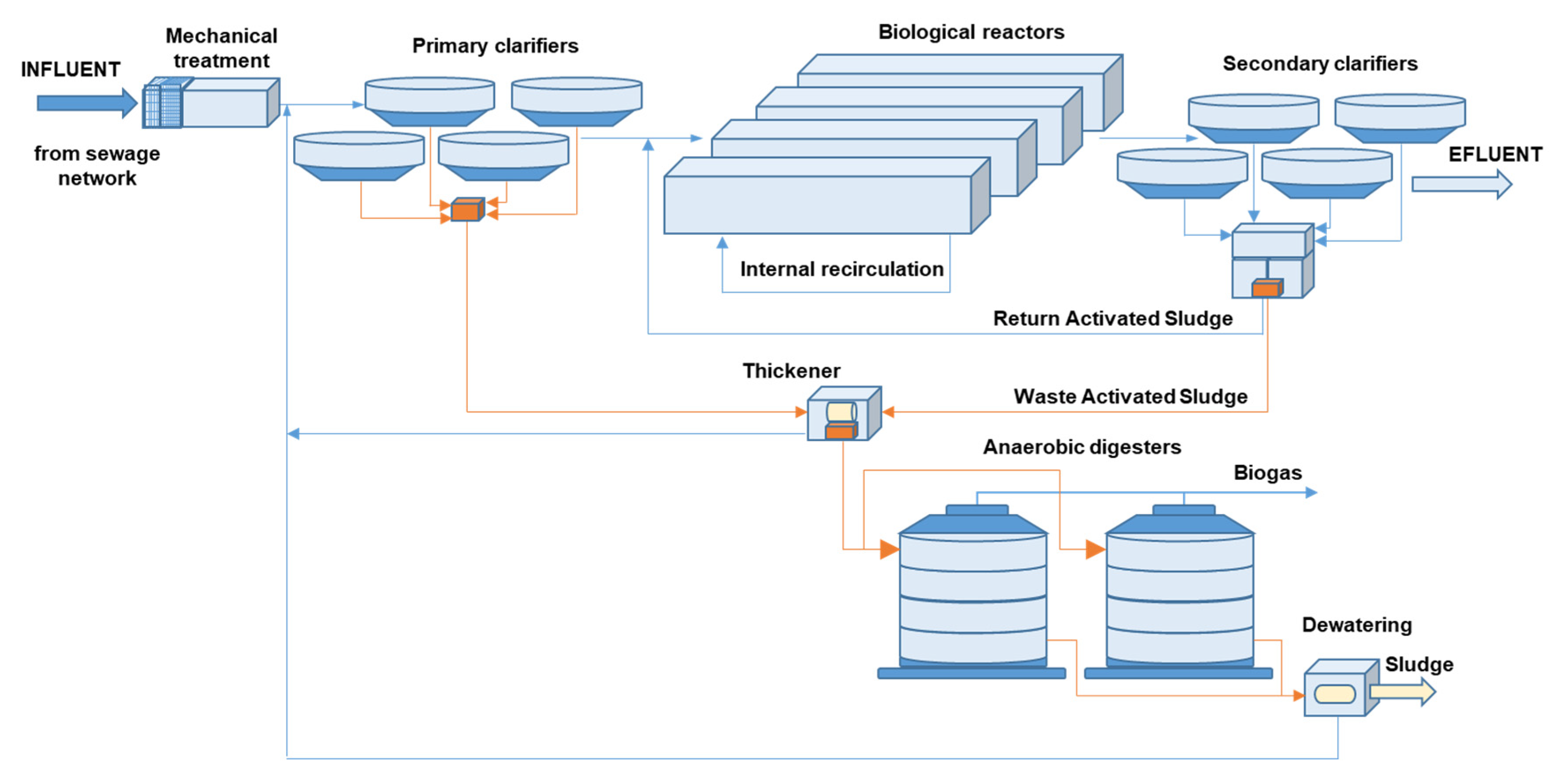
2.1. Structure of the Wastewater Treatment Plant

Figure 1 shows a global view of the treatment plant of Galati city. It contains the following three systems: 1. mechanical treatment, 2. biological treatment and 3. sludge treatment. The biological treatment subsystem consists of four identical treatment lines, as it can be seen in Figure 1.
Figure 2 presents schematically the structure of one of the four biological treatment lines, together with the automation equipment. In order to exemplify the proposed control method, only one biological treatment line was considered in the paper.
Regarding the anaerobic digestion system, it was considered a single anaerobic digester with a capacity equal to half that of a real one. The treatment plant was modeled in SIMBA by the ASM1 model and for the anaerobic digester the model ADM1 was used.
The tank capacities of the wastewater treatment plant are given in Table 1:

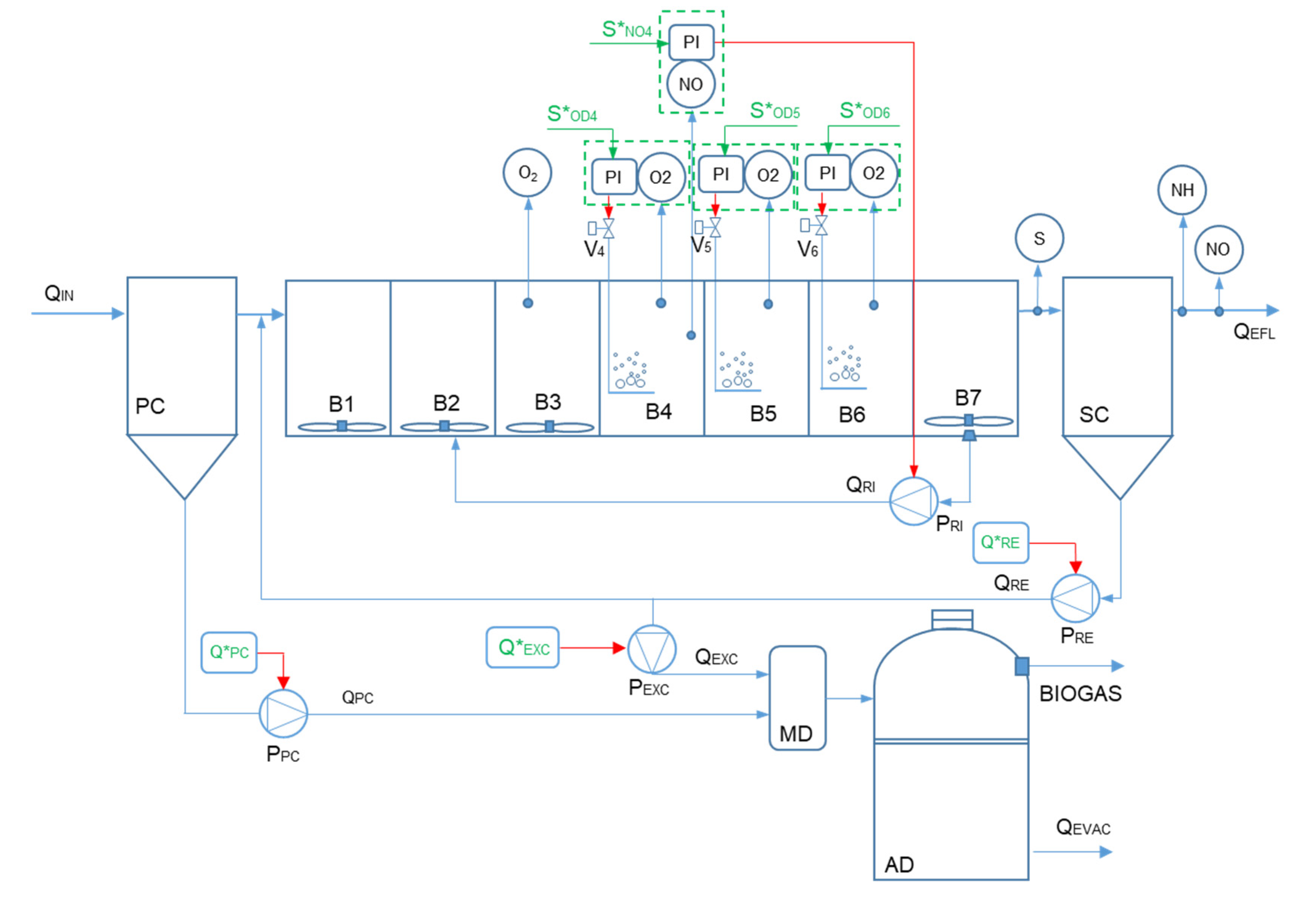
2.2. Automation Equipment

The main automation equipment of the wastewater treatment process can be seen in Figure 2. It consists in the following elements:
  • dissolved oxygen concentration loops in the tanks B4, B5 and B6;
  • nitrate concentration control loop through internal recirculation. From the last tank—B7—the sludge is recirculated by a pumping group to the second tank, B2;
  • the pump that ensures the sludge flow extracted from the primary clarifier ( Q P C * );
  • the pump that ensures the sludge flow for the external recirculation ( Q R E * );
  • the pump that determines the excess sludge flow from the secondary clarifier ( Q E X C * ).
There are several solutions regarding the aeration system in the literature [37]. In this case, the air is supplied in the aeration tanks by means of four blowers powered by frequency converters. The pressure in the output collector of the blowers is maintained at a value imposed by the variation of their speed and the number of blowers in operation. The air is released in tanks using fine bubble membrane diffusers, located at the bottom of the aerated tanks. The dissolved oxygen concentration is controlled using control valves mounted on the distribution network for each tank separately.
Dissolved oxygen concentration control loops in the tanks B4, B5 and B6 and the nitrate concentration control loop are based upon PI controllers. All these control loops include anti-windup sequences aiming at limiting the effect of the integrator component of the controller when technological operating limitations of the actuators are imposed. Controllers’ parameters are tuned similarly with those used in BSM2, according to the methodology presented in [31].

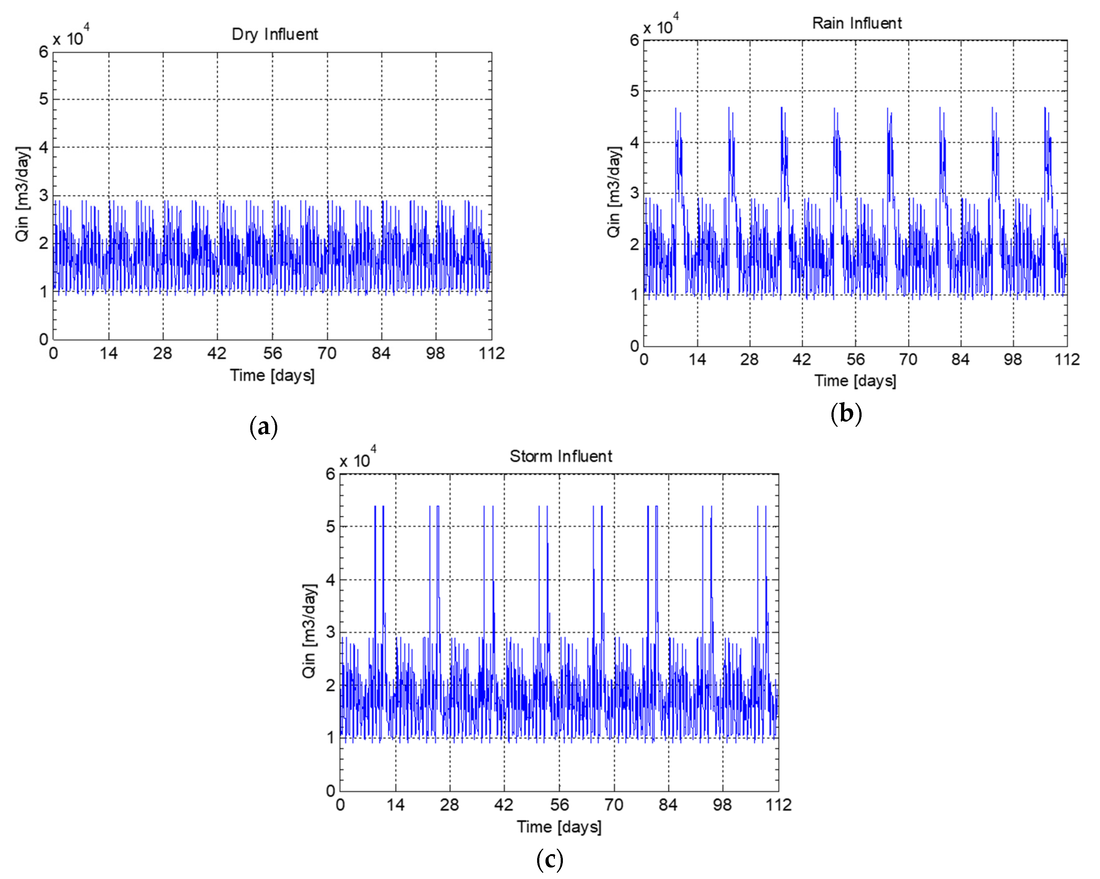
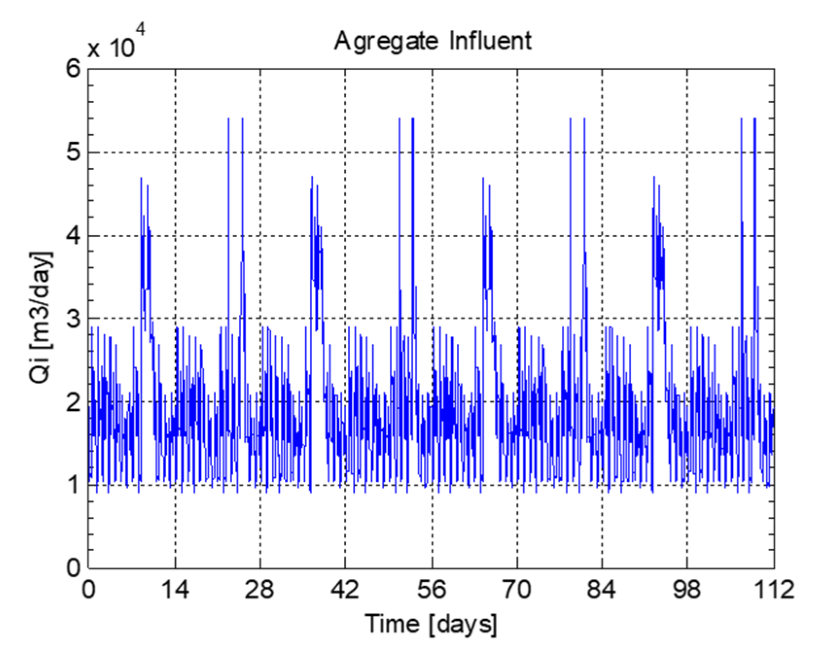
2.3. The Influent Used in Simulations

The influent was obtained based on the one from BSM1 benchmark. It was calibrated to the loads specific to Galati city treatment plant by linear transformations for each operating regime. The influent takes into account the diurnal variations, as well as the week-end ones, of the flow and loads specific to Galati city. Table 2 presents the plant design values and the measured average values over 2017. It should be mentioned that three measurements per day are made in the laboratory, then from these measurements monthly and then annual averages are calculated:
The inflow average values corresponding to the three operating regimes are as follows: Q i n , D R Y = 16 , 601 m3/day, Q i n , R A I N = 19 , 188 m3/day and Q i n , S T O R M = 17 , 771 m3/day.
Thus, three files of influent were created in order to determine the optimal setpoint for each operating regime. Figure 3 presents the inflow variations in the three operating regimes over a period of 112 days (16 weeks) of which in 12 weeks the entire system reaches the steady state regime and the last 4 are used to evaluate the process performance. Cyclical data over a longer period of time with RAIN and STORM events are disturbances that seriously stress the system and show its limitations and the context in which the parameter values exceed the legal limits.
In order to test global operation of the wastewater treatment plant, a fourth file of influent was created by suitably aggregating sequences corresponding to the three operating regimes. It was created over the same period of 16 weeks and includes a succession of regimes DRY, RAIN and STORM regimes. Figure 4 presents the aggregated influent. The membership to the current operating regime is determined through a fuzzification block.

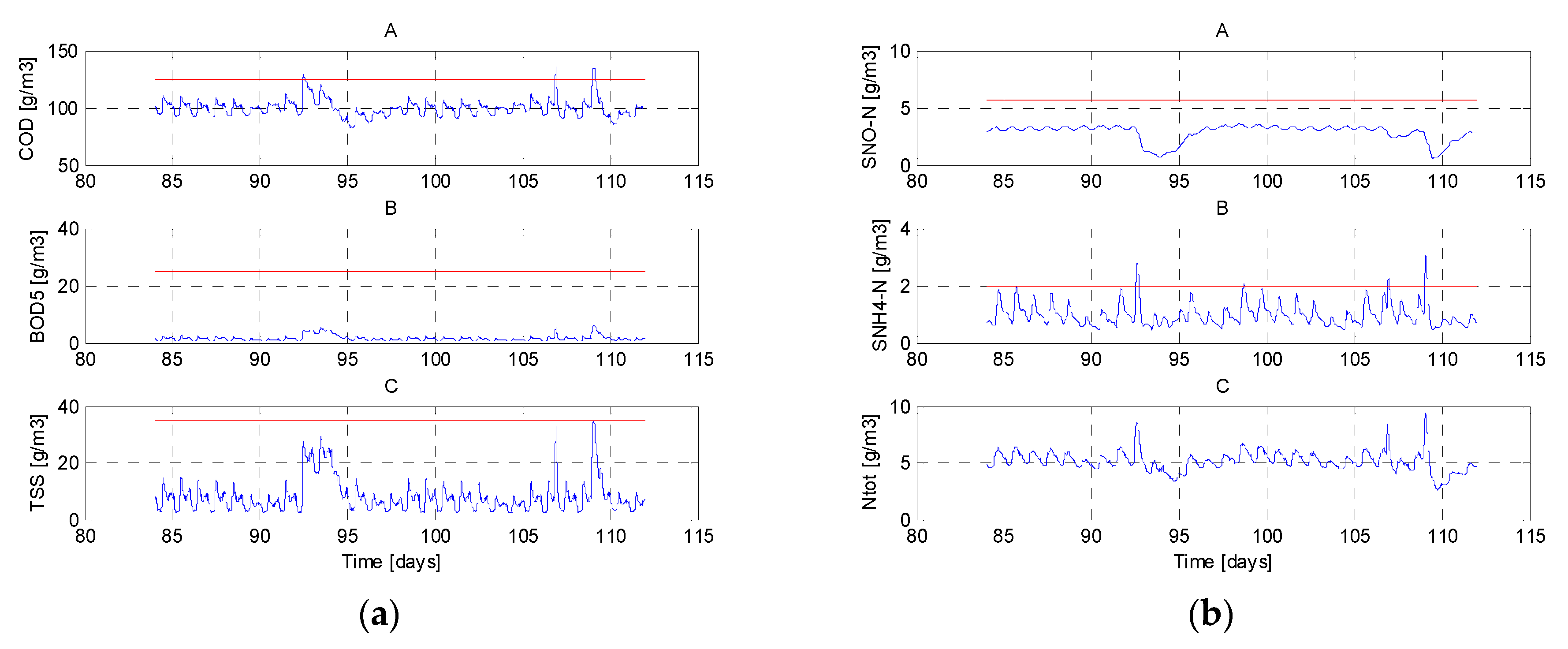
2.4. Performance Criterion Regarding the Efficiency of the Wastewater Treatment Plant

The performance evaluation of the control strategy was performed using the indicators defined in BSM2, because it includes the model of the anaerobic digester, similar to the model considered in this paper [16]. The performance criterion used to optimize the operation of the wastewater treatment plant has three components:
  • Effluent quality (EQI)—J1
    J 1 =   1 T · 1000     t 1   = 84   d a y s t 2   = 112   d a y s ( B S S ·   T S S e ( t ) + B C O D · C O D e ( t ) + B N K j · S N K j , e ( t ) + B N O , e · S N O , e ( t ) + B B O D 5 · B O D e ( t ) ) d t ,
    where T = t2t1 represents the total evaluation period, in our case 28 days, between days t1 = 84 and t2 = 112. The weighting coefficients B S S , B C O D , B N K j , B N O , e and B B O D 5 are used to convert the effluent loads into pollution units. The values of these coefficients were taken from [16], having the following values: B S S = 2 , B C O D = 1 , B N K j = 30 , B N O , e = 10 , and B B O D 5 = 2 .
  • Overall cost index (OCI)—J2
    J 2 = A E + P E + 3 · S P + M E 6 · M E T p r o d ,
    where AE represents the Aeration Energy, PE—the Pumping Energy, SP—Total Sludge Production, ME—Mixing Energy and METprod—Methane production [16,31].
  • “Failure” index—J3
    J 3 = E x   _   [ N t o t + N H 4 + T S S + C O D + B O D 5 ]
  • where Ex—percentage exceeding of the legal limits over the last 28 days.
  • In this paper an aggregated performance criterion was considered:
    J = α 1 · J 1 + α 2 · J 2 + α 3 · J 3
    where α1, α2, α3 are weighting coefficients. They have the following values: α1 = 0.5, α2 = 1 and α3 = 100. They were chosen taking into account the size orders of the indexes J1J3 so as to ensure a balanced contribution in the global indicator J.

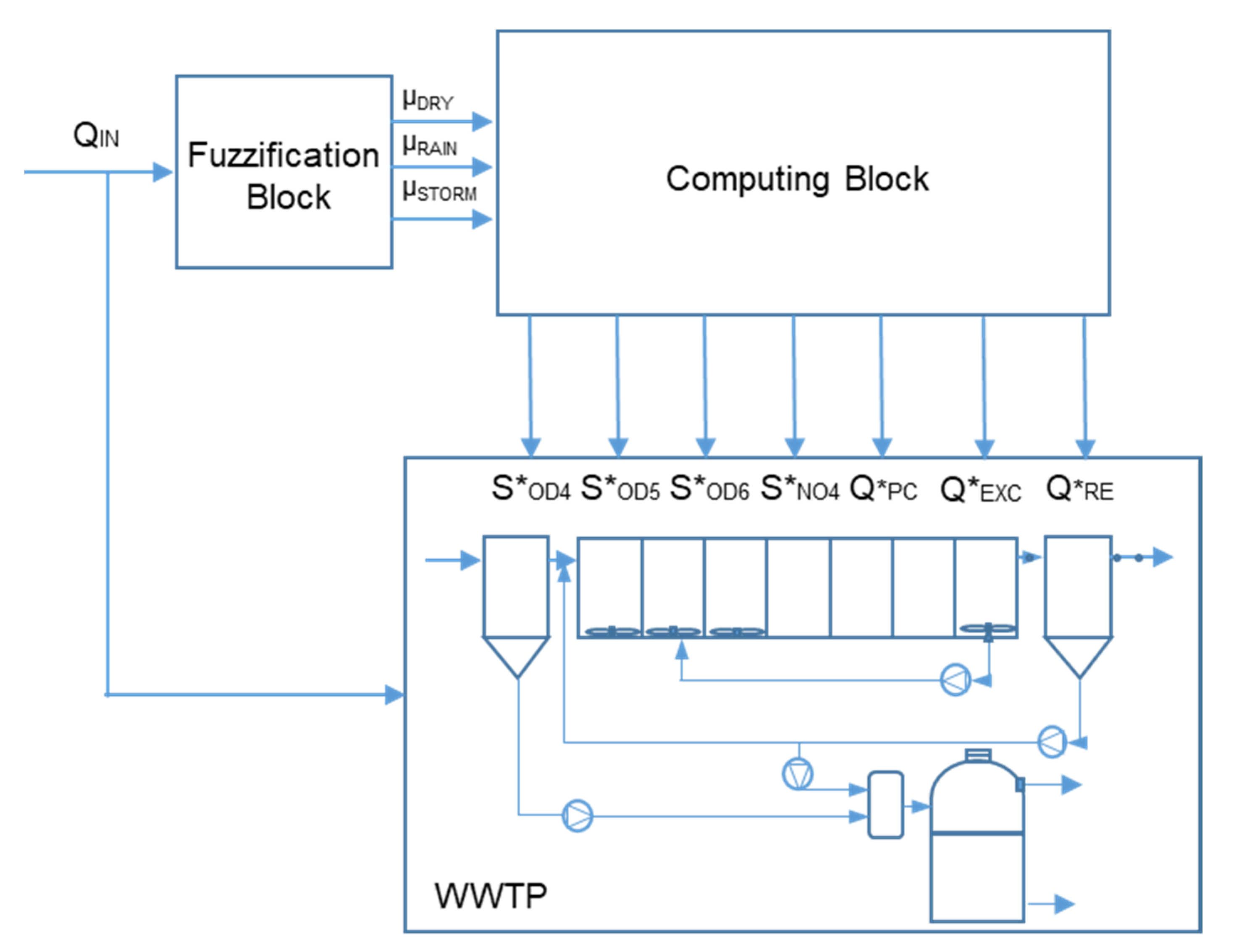
2.5. Control Strategy

The control strategy has two stages:
  • computation of the optimal setpoint set for operating regimes;
  • obtaining the current optimal setpoint set for the current operating regime or, in the case of transitions between regimes, taking into account the membership to the operating regime through a fuzzification block.

2.5.1. Computation of the Optimal Setpoints for Operating Regimes

For each operating regime, the vector of the optimal setpoints is calculated:
V i * = [ S O D 4 , i * , S O D 5 , i * , S O D 6 , i * , S N O 4 , i * , Q R E , i * , Q P C , i * , Q E X C , i * ] T ,   i { D R Y ,   R A I N , S T O R M }
where S O D 4 , i * —setpoint of the dissolved oxygen concentration in the tank B4, S O D 5 , i * —setpoint of the dissolved oxygen concentration in the tank B5, S O D 6 , i * —setpoint of the dissolved oxygen concentration in the tank B5, S N O 4 , i * —setpoint of the nitrate concentration, Q R E , i * —external recirculation flow, Q P C , i * —the sludge flow extracted from the primary clarifier and Q E X C , i * —the excess sludge flow from the secondary clarifier.
It is considered that the recirculation flow depends proportionally on the inflow Qin:
Q R E , i * = k R E , i * · Q i n ,   i { D R Y ,   R A I N , S T O R M }
The optimal setpoint vector becomes:
V i * = [ S O D 4 , i * , S O D 5 , i * , S O D 6 , i * , S N O 4 , i * , k R E , i * , Q P C , i * , Q E X C , i * ] T ,   i { D R Y ,   R A I N , S T O R M }
Further on the optimal setpoint vector is determined by minimizing the performance criterion J, defined by the Equation (4):
J * = min V J
A genetic algorithm was used for the minimization of the performance criterion J. Within genetic algorithm the chromosomes contain 7 genes, these being exactly the searched setpoints, which are the components of the vector V*, given by Equation (5). The genetic algorithm was implemented in Matlab and its main characteristics are given in Appendix A.

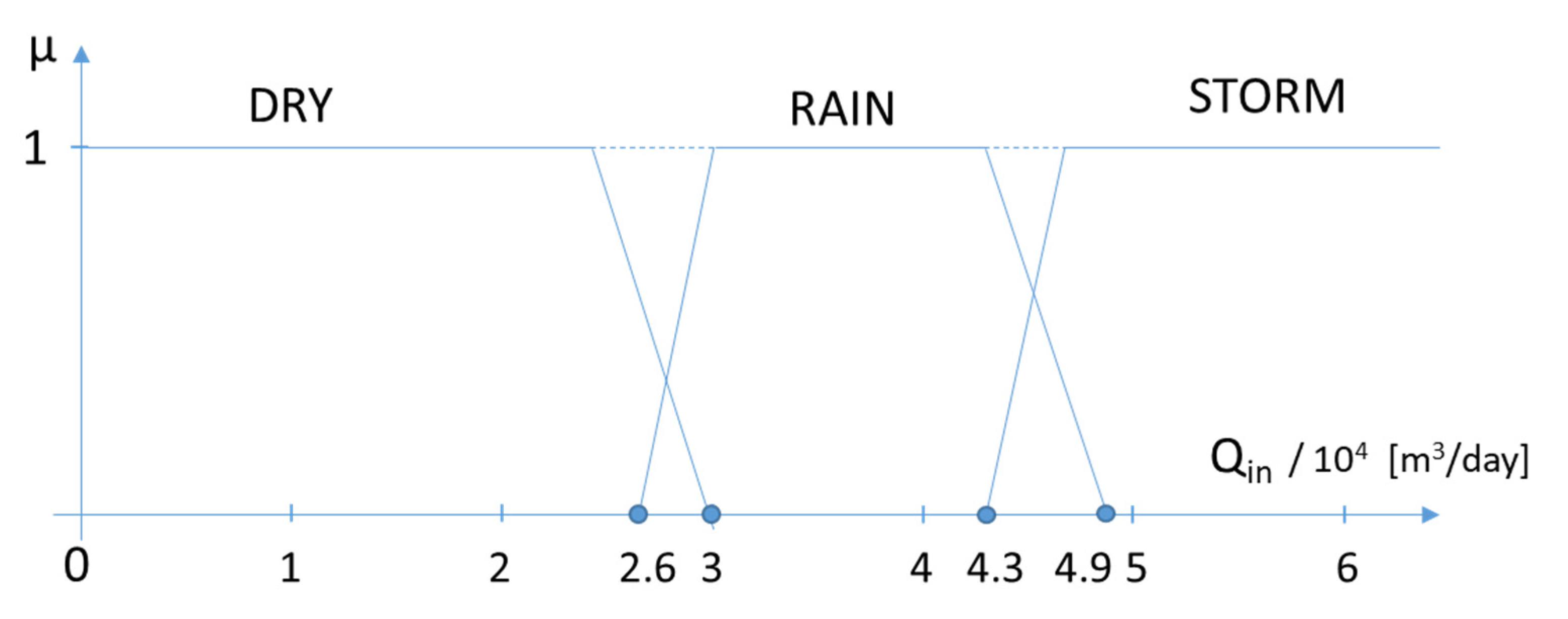
2.5.2. Computation of the Current Optimal Setpoint Set for the Current Operating Regime or in the Case of Transitions between Regimes

Figure 5 presents the control strategy of the wastewater treatment plant. It derives from Figure 2 to which two additional blocks were added: 1. a fuzzification block for determining the Qin membership to the current operating regime and 2. a computation block of the current setpoints.
The role of the fuzzification block is to achieve a smooth transition between the operating regimes of the wastewater treatment plant. Figure 6 presents the membership functions regarding the membership to the current operating regime (the maximum limit of the considered inflow is 55,000 m3/day—see Figure 4). The main idea of using the fuzzification block is to provide the membership degrees of Qin to the current operating regime. This membership degree further serves at computing the setpoints that will actually be applied in the wastewater treatment process.
Finally, the optimal setpoint vector—V—which results from the computing block (on the seven components) is given by the following equation:
V * [ j ] = i μ i · V i * [ j ] ,   j = 1 7 ,   i { D R Y ,   R A I N , S T O R M }
That means
S O D 4 * = i μ i · S O D 4 , i *
S O D 5 * = i μ i · S O D 5 , i *
S O D 6 * = i μ i · S O D 6 , i * ,
S N O 4 * = i μ i · S N O 4 , i * ,
k R E * = i μ i · k R E , i * ,
Q P C * = i μ i · Q P C , i * ,
Q E X C * = i μ i · Q E X C , i * ,
where μ i represents the membership degree at the operating regime i, i { D R Y ,   R A I N , S T O R M } .

3. Results and Discussions

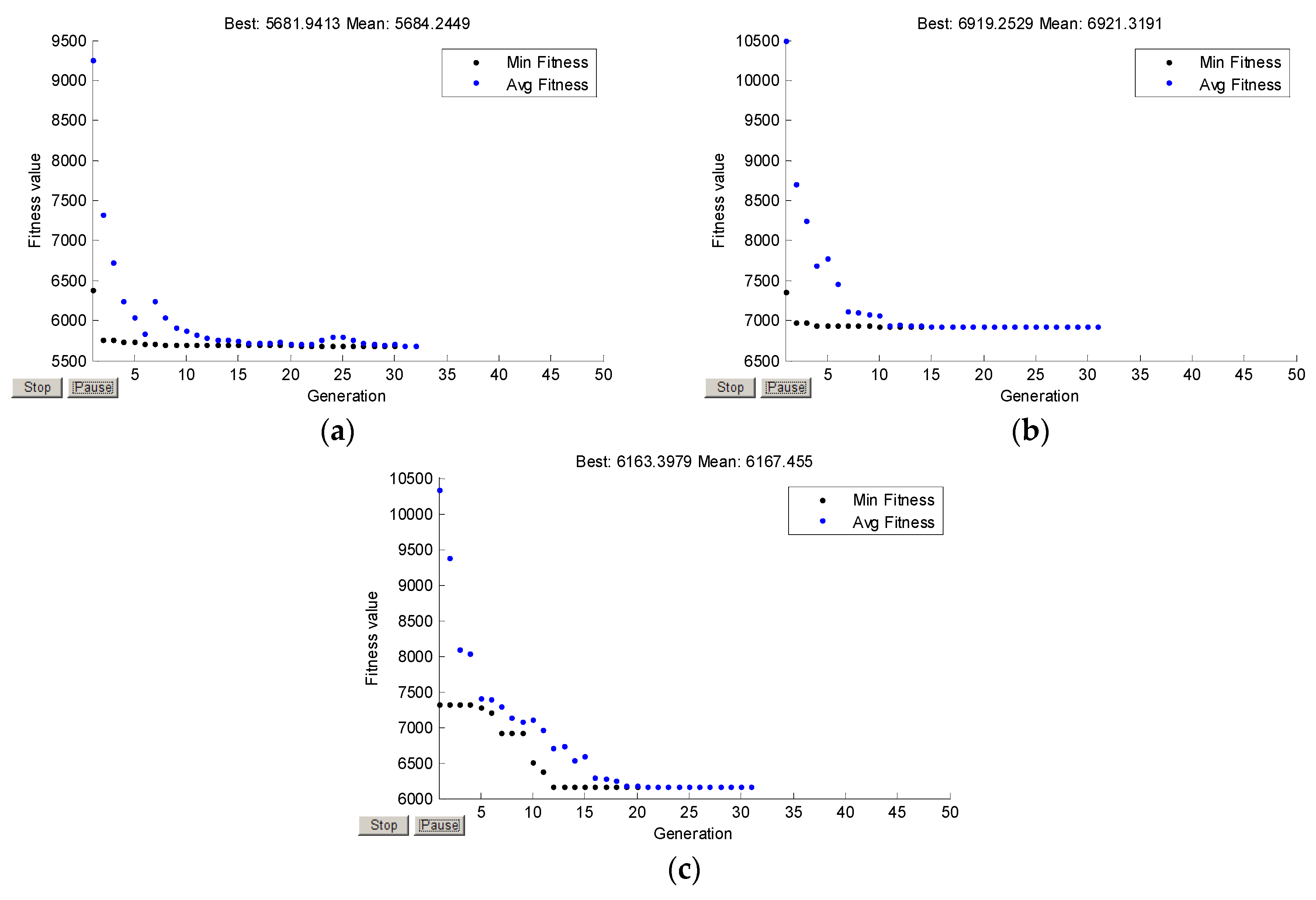
3.1. Computation of the Optimal Setpoints for Each of the Three Operating Regimes

As mentioned in the previous section, a genetic algorithm was used for the computation of the optimal setpoints in the three operating regimes. For technological reasons, the initial population for starting the genetic algorithm was chosen in the intervals indicated in Table 3.
Table 4 presents the optimal setpoints obtained with the genetic algorithm.
The influent files from Figure 3 (a: DRY, b: RAIN and c: STORM) were used to calculate the optimal setpoints. Simulation was performed on a 112-day time horizon and the performance criteria were evaluated on the last 28 days. The results can be seen in Table 5:
In Table 5, IQI represents the influent quality. It is calculated similarly to EQI using influence loads and the weighting coefficients are identical to those used in EQI. Ex indicates the percentage exceeding of the main quality parameters of the influent, whereas J1, J2, J3 and J were defined in Section 2.4. The efficiency of the treatment plant is expressed by the quality index of the effluent being approximately 10 times lower than that of the influent. It can also be noticed that there are a series of exceeding RAIN and STORM regimes of the variables’ total nitrogen, ammonium and COD, whose amounts are sufficiently low. The highest value of criterion J is obtained in the case of the RAIN operating regime. All the three criteria contribute to this fact, as expected, due to the increased flow of the influent that characterizes the RAIN operating regime.
Figure 7 shows screenshots from the genetic algorithm running program, where the evolution of the fitness functions in the case of the three operating regimes can be noticed.

3.2. Computation of the Current Optimal Setpoint Set for the Current Pluviometric Regime or in the Case of Transitions between Regimes

In this case, the influent file from Figure 4 was considered to validate the control strategy. In reality, the transition from one operating regime to another is not net but gradual. This is the reason why it is reasonable to take into account these transitions by weighting the optimal setpoints in each operating regime by the membership to the operating regimes.
To this end, the simulation scheme includes a fuzzification block and a computing one of the setpoints taking into account the membership to the current operating regime of the treatment plant (see Figure 5). The simulation time horizon was identical to the one in the previous section. The results are presented in Table 6.
Figure 8 shows the loads of the effluent main quality parameters over the time horizon between day 84 and day 112 (last 28 of the 112 days of simulation), considering the aggregate influent. The red line marked maximum limits stipulated by Romanian legislation (NTPA 011—The normative regarding the load limits with pollutants of industrial and urban wastewater at the discharge in natural receivers). These are the following: COD = 125 mg/L, BOD5 = 25 mg/L, TSS = 35 mg/L, Ntot = 10 mg/L, SNH4-N= 2 mg/L and SNO-N = 5.65 mg/L. The graphs show the limit exceeding of COD and ammonium; exceeding of the same variables are also observed in Table 6 (1.75%—COD and respectively 1.29%—ammonium concentration). The moments of exceeding coincide with those when the influent flow reaches maximum values in RAIN and STORM regimes.

4. Conclusions

In this paper, a control strategy for a wastewater treatment plant is proposed, which is based on the optimization of the control loops’ setpoints, so that it operates in an optimal operating point. The objective of the control system is the decrease of nitrogen concentration and its components in the effluent in conditions of minimum energy consumption. This strategy was validated in numerical simulation on an activated sludge mathematical model, built in SIMBA and calibrated on the dimensions of a real treatment plant. The results were obtained considering an influent similar to that from BSM 1 at the plant input and calibrated to the specific values of the real treatment plant. The search of the optimal setpoints for each pluviometric regime was performed with a genetic algorithm that provides seven variables (three setpoints of the dissolved oxygen concentration in the aerated tanks, the setpoint of the nitrate concentration, the external recirculation flow, the sludge flow extracted from the primary clarifier and the excess sludge flow from the secondary clarifier). For the calculation of the setpoints that are applied directly in the process, a fuzzification block was used, which takes into account the membership to the current pluviometric regime.
The obtained results showed an improvement of the treatment plant performances. Thus, the pollutant loading of the effluent was reduced about 10 times compared to that of the influent (the effluent quality index—EQI is about ten times lower than that of the influent—IQI). Furthermore, the genetic algorithm proves to be efficient in the sense that it finds the minimum of criterion J accurately enough. The lowest value of the performance criterion J is obtained in the case of the DRY operating regime. Higher values of J are obtained in STORM and RAIN operating regimes, this being due to the increased values of the influent flow, Qin. In the case of the aggregate influent, an intermediate value of the performance criterion J is obtained, which was to be expected, because the influent used for the validation method contains sequences of all the three operating regimes. In the DRY operating regime, none of the effluent main quality parameters exceeds the admissible limits and, therefore, criterion J3 is zero. On the other hand, there are a number of limits exceeding COD and ammonium concentration in RAIN and STORM operating regimes at the moments when a number of peaks are observed in the evolution of Qin. This exceeding causes, in the RAIN and STORM regimes, the criterion J3 to be different from zero, contributing to the worsening of the aggregate criterion J. Last but not least, the actuators of the treatment plant have an easier operating regime due to the use of the fuzzification block which makes a smooth transition from one operating regime to another.
Further on the authors intend to apply the control strategy presented in the paper within the real wastewater treatment plant. It is also intended to continue research considering other basic control loop configurations within a wastewater treatment process (for example, extending the treatment process by including the phosphorus removal).

Author Contributions

Conceptualization, S.C.; Writing—original draft preparation, S.C.; Design and simulation of mathematical model and control algorithm, L.L.; Design of genetic algorithm, I.V.; Results validation, M.B. All authors have read and agreed to the published version of the manuscript.

Funding

This work is supported by the project “EXPERT”, Contract No. 14PFE/17.10.2018.

Conflicts of Interest

The authors declare no conflict of interest.

Appendix A

The genetic algorithm used to calculate the optimal setpoints for each operating regime has the following characteristics:
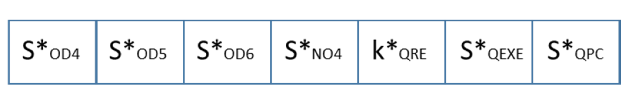
  • a chromosome consists of seven genes being exactly the searched setpoints, which are the components of the vector V*, given by (5) (see Figure A1);
    Figure A1. Chromosome structure.
    Figure A1. Chromosome structure.
    Processes 08 01203 g0a1
  • for the generation of the initial population, searching intervals of the optimal solution are chosen (see Table 3). Their choice was made upon technological considerations;
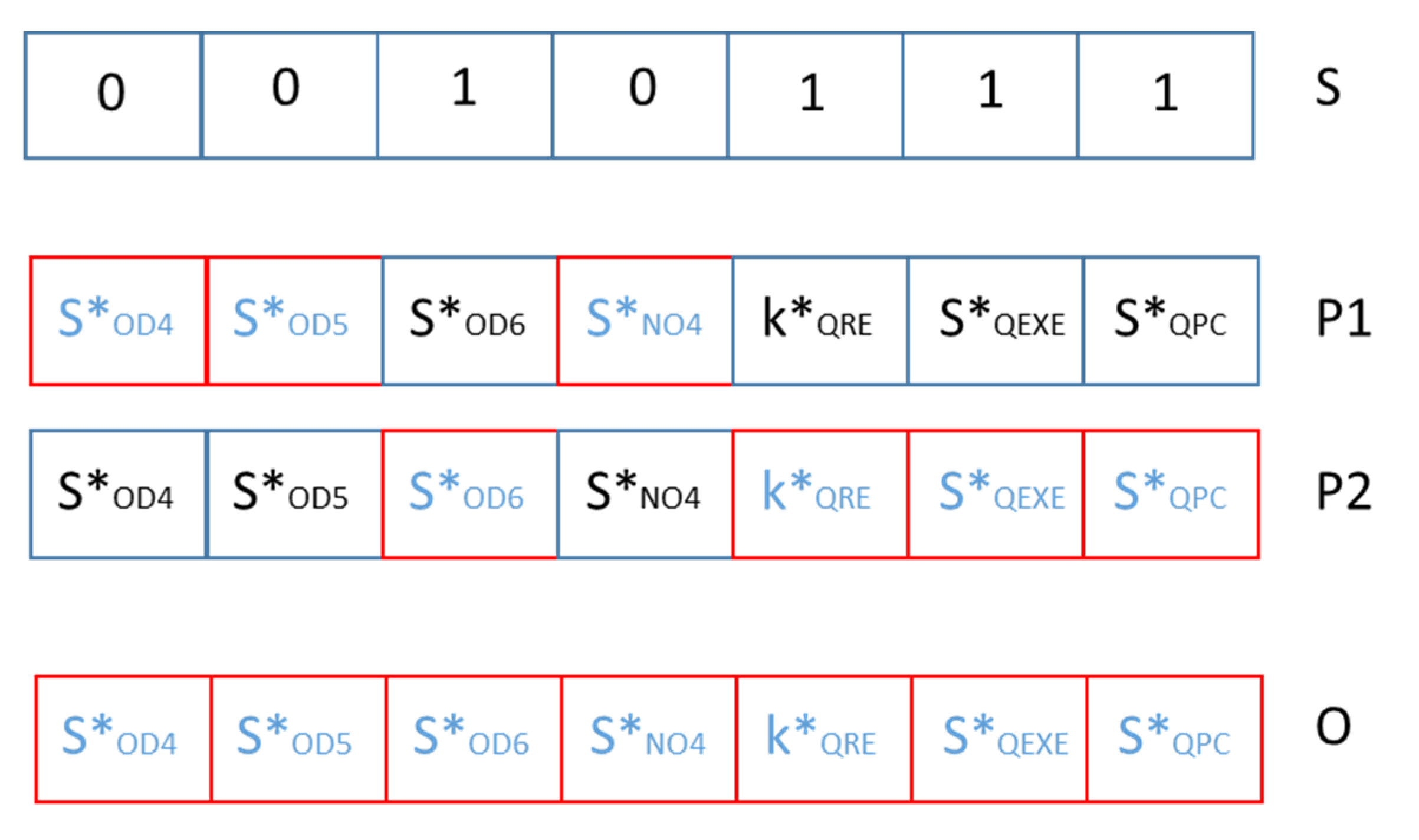
  • an offspring chromosome (O) is obtained from two parent chromosomes (P1 and P2). For crossover a binary vector was used, having the same length as that of a chromosome whose values will be randomly chosen. Let us denote this vector by S. Once this vector is generated, each gene k of offspring chromosome will inherit the value of gene k of the first parent if S(k) = 0 or the value of gene k of the second parent if S(k) = 1, according to Figure A2;
    Figure A2. Crossover operation.
    Figure A2. Crossover operation.
    Processes 08 01203 g0a2
  • selection of the parent chromosomes is made randomly, with a probability inversely proportional to the value of the offspring chromosome’s fitness function. Thus, chromosomes with the low fitness function are more likely to be selected as parents;
  • the mutation operator adds to each parent gene a randomly chosen value from a Gaussian distribution with zero mean and standard deviation calculated for each gene according to the relation:
    σ k = σ k 1 · ( 1 k G e n ) ,
    where
    • k—number of the current generation.
    • Gen—total number of generations for which the algorithm is run.
    • σ k —standard deviation of the Gaussian distribution at generation k.
    • σ 1 —standard deviation at the first generation—has the value equal to the size of the gene range that undergoes mutation (for example, S O D 4 * varies between 0.4 and 4, so for this gene σ 1 = 4 0.4 = 3.6 ).
For the next generation only the best N chromosomes are selected, where N is the population dimension.

References

  1. Council of the European Communities (CEC). Directive concerning urban wastewater treatment (91/271/EEC). Off. J. Eur. Commun. 1991, 34, 40. [Google Scholar]
  2. DCE. “Directive 2000/60/CE du Parlement européen et du Conseil du 23 octobre 2000 établissant un cadre pour une politique communautaire dans le domaine de l’eau. J. Off. 2001, 327, 0001–0073. [Google Scholar]
  3. Jeppsson, U. Modelling Aspects of Wastewater Treatment Processes. Ph.D. Thesis, Lund Institute of Technology, Lund, Sweden, 1996. [Google Scholar]
  4. Yang, Y.Y.; Linkens, D.A. Modelling of Continuous Bioreactors via Neural Networks. Trans. Inst. Meas. Control 1993, 15, 158–169. [Google Scholar] [CrossRef]
  5. Barbu, M.; Caraman, S.; Ifrim, G.; Bahrim, G.; Ceanga, E. State observers for food industry wastewater treatment processes. J. Environ. Prot. Ecol. 2011, 12, 678–687. [Google Scholar]
  6. Katebi, M.R.; Johnson, M.A.; Wilke, J. Control and Instrumentation for Wastewater Treatment Plant; Springer: London, UK, 1999. [Google Scholar]
  7. Olsson, G.; Newell, B. Wastewater Treatment Systems—Modelling, Diagnosis and Control; IWA Publishing: London, UK, 1999. [Google Scholar]
  8. Dochain, D.; Vanrolleghem, P. Dynamical Modeling & Estimation in Wastewater Treatment Processes; IWA Publishing: London, UK, 2001. [Google Scholar]
  9. Henze, M.; Grady, C.P.L., Jr.; Gujer, W.; Marais, G.V.R.; Matsuo, T. Activated Sludge Model No. 1; IAWQ Scientific and Technical Report No. 1; IAWQ: London, UK, 1987. [Google Scholar]
  10. Henze, M.; Gujer, W.; Mino, T.; Matsuo, T.; Wentzel, M.C.; Marais, G.V.R. Activated Sludge Model No. 2; IAWQ Scientific and Technical Report No. 3; IAWQ: London, UK, 1995. [Google Scholar]
  11. Henze, M.; Gujer, W.; Mino, T.; van Loosdrecht, M. Activated Sludge Models AMS1, ASM2, ASM2d and ASM3, IWA STR No. 9; IWA Publishing: London, UK, 2000. [Google Scholar]
  12. Batstone, D.; Keller, J.; Angelidaki, I.; Kalyuzhnyi, S.; Pavlostathis, S.; Rozzi, A.; Sanders, W.; Siegrist, H.; Vavilin, V. The IWA Anaerobic Digestion Model No 1 (ADM1). Water Sci. Technol. 2002, 45, 65–73. [Google Scholar] [CrossRef] [PubMed]
  13. Batstone, D.J.; Keller, J. Industrial applications of the IWA anaerobic digestion model No.1 (ADM1). Water Sci. Technol. 2003, 47, 199–206. [Google Scholar] [CrossRef] [Green Version]
  14. Nejjari, F.; Dahhou, B.; Benhammou, A.; Roux, G. Non-linear multivariable adaptive control of an activated sludge wastewater treatment process. Int. J. Adapt. Control Signal Process. 1999, 13, 347–365. [Google Scholar] [CrossRef]
  15. Boger, Z. Application of neural networks to water and wastewater treatment plant operation. ISA Trans. 1992, 31, 25–33. [Google Scholar] [CrossRef]
  16. Jeppsson, U.; Pons, M.-N.; Nopens, I.; Alex, J.; Copp, J.B.; Gernaey, K.V.; Rosen, C.; Steyer, J.-P.; Vanrolleghem, P.A. Benchmark Simulation Model No 2 – General protocol and exploratory case studies. Water Sci. Technol. 2007, 56, 67–78. [Google Scholar] [CrossRef]
  17. Alex, J.; Benedetti, L.; Copp, J.B.; Gernaey, K.V.; Jeppsson, U.; Nopens, I.; Pons, M.-N.; Rosen, C.; Steyer, J.-P.; Vanrolleghem, P. Benchmark Simulation Model No 1, Prepared by the IWA Taskgroup on Benchmarking of Control Stategies for WWTPs; Department of Industrial Electrical Engineering and Automation, Lund University: Lund, Sweden, 2008. [Google Scholar]
  18. Vrecko, D.; Gernaey, K.V.; Rosen, C.; Jeppsson, U. Benchmark simulation model No 2 in Matlab-Simulink: Towards plant-wide WWTP control strategy evaluation. In Proceedings of the IWA World Water Congress, Beijing, China, 10–14 September 2006. [Google Scholar]
  19. Chirosca, A.; Luca, L.; Ifrim, G.; Caraman, S. Robust control of the biological wastewater treatment process. In Proceedings of the 2013 17th International Conference on System Theory, Control and Computing, ICSTCC 2013, Joint Conference of SINTES 2013, SACCS 2013, SIMSIS 2013, Sinaia, Romania, 11–13 October 2013. [Google Scholar]
  20. Brdys, M.A.; Zhang, Y. Robust Hierarchical Optimizing Control of Municipal Wastewater Treatment Plants. In Proceedings of the 9th IFAC/IFORS/IMACS/IFIP Symposium Large Scale Systems: Theory & Applications, Bucharest, Romania, 18–20 July 2001; pp. 540–547. [Google Scholar]
  21. Georgieva, P.G.; de Azevedo, S.F. Robust control design of an activated sludge process. Int. J. Robust Nonlinear Control 1999, 9, 949–967. [Google Scholar] [CrossRef]
  22. Luca, L.; Barbu, M.; Ifrim, G.; Ceangă, E.; Caraman, S. Control Strategies of a Wastewater Treatment Plant. In Proceedings of the 12th IFAC Symposium on Dynamics and Control of Process Systems, Including Biosystems, Florianopolis, Brazil, 23–26 April 2019. [Google Scholar]
  23. Caraman, S.; Sbarciog, M.; Barbu, M. Predictive control of a wastewater treatment process. IFAC Proc. Vol. 2006, 39, 155–160. [Google Scholar]
  24. Mulas, M.; Tronci, S.; Corona, F.; Haimi, H.; Lindell, P.; Heinonen, M.; Vahala, R.; Baratti, R. Predictive control of an activated sludge process: An application to the Viikinmäki wastewater treatment plant. J. Process Control 2015, 35, 89–100. [Google Scholar]
  25. Bastin, G.; Dochain, D. On-Line Estimation and Adaptive Control of Bioreactors; Elsevier: Amsterdam, The Netherlands, 1990. [Google Scholar]
  26. Guerrero, J.; Guisasola, A.; Vilanova, R.; Baeza, J.A. Improving the performance of a WWTP control system by model-based setpoint optimization. Environ. Model. Softw. 2011, 26, 492–497. [Google Scholar]
  27. Luca, L.; Ifrim, G.; Ceanga, E.; Caraman, S.; Barbu, M.; Santin, I.; Vilanova, R. Optimization of the Wastewater Treatment Processes Based on the Relaxation Method; ISEEE: Galati, Romania, 2017. [Google Scholar]
  28. Xu, H.; Vilanova, R. PI and fuzzy control for P-removal in wastewater treatment plant. Int. J. Comput. Commun. Control 2015, 10, 176. [Google Scholar]
  29. Santín, I.; Pedret, C.; Vilanova, R.; Meneses, M. Advanced decision control system for effluent violations removal in wastewater treatment plants. Control Eng. Pract. 2016, 49, 60–75. [Google Scholar]
  30. Manesis, S.A.; Sapidis, D.J.; King, R.E. Intelligent Control of Wastewater Treatment Plants. Artif. Intell. Eng. 1998, 12, 275–281. [Google Scholar]
  31. Laurentiu, L. Advanced Control Strategies for Biological Waste Water Treatment Processes. Ph.D. Thesis, Galati University Press, Galati, Romania, 2018. [Google Scholar]
  32. Piotrowski, R.; Skiba, A. Nonlinear Fuzzy Control System for Dissolved Oxygen with Aeration System in Sequencing Batch Reactor. Inf. Technol. Control 2015, 44, 182–195. [Google Scholar]
  33. Piotrowski, R.; Błaszkiewicz, K.; Duzinkiewicz, K. Analysis the Parameters of the Adaptive Controller for Quality Control of Dissolved Oxygen Concentration. Inf. Technol. Control 2016, 45, 42–51. [Google Scholar]
  34. Piotrowski, R.; Lewandowski, M.; Paul, A. Mixed integer nonlinear optimization of biological processes in wastewater sequencing batch reactor. J. Process Control 2019, 84, 89–100. [Google Scholar]
  35. Piotrowski, R.; Paul, A.; Lewandowski, M. Improving SBR performance alongside with cost reduction through optimization of biological processes and dissolved oxygen concentration trajectory. Appl. Sci. 2019, 9, 2268. [Google Scholar]
  36. Hirsch, P.; Piotrowski, R.; Duzinkiewicz, K.; Grochowski, M. Supervisory Control System for Adaptive Phase and Work Cycle Management of Sequencing Wastewater Treatment Plant. Stud. Inform. Control 2016, 25, 153–162. [Google Scholar] [CrossRef]
  37. Piotrowski, R.; Brdys, M.A.; Konarczak, K.; Duzinkiewicz, K.; Chotkowski, W. Hierarchical dissolved oxygen control for activated sludge processes. Control Eng. Pract. 2008, 16, 114–131. [Google Scholar] [CrossRef]
Figure 1. The general scheme of the wastewater treatment plant of Galati city.
Processes 08 01203 g001
Figure 2. Schematic representation of a treatment line together with the automation equipment.
Processes 08 01203 g002
Figure 3. Inflow variations corresponding to the three operation regimes (a) DRY; (b) RAIN; (c) STORM.
Processes 08 01203 g003
Figure 4. Sequence of operating regimes used in simulations.
Processes 08 01203 g004
Figure 5. The proposed control strategy of the wastewater treatment plant.
Processes 08 01203 g005
Figure 6. Membership functions of Qin to the operating regimes.
Processes 08 01203 g006
Figure 7. Fitness functions in the case of the three operating regimes: (a) DRY; (b) RAIN; (c) STORM.
Processes 08 01203 g007
Figure 8. Loads of the effluent quality parameters: (a) COD, BOD5, TSS; (b) SNO-N, SNH4-N, Ntot.
Processes 08 01203 g008
Table 1. The tank capacities of a wastewater treatment plant.
Type of the TankCapacity (m3)
Primary clarifier (PC)3300
Anoxic tank (B1)1200
Anoxic tank (B2)2200
Aerated tank (B3 and B4)2200
Aerated tank (B5 and B6)3300
Deaeration tank (B7)500
Secondary clarifier (SC)9200
Anaerobic digester (AD)6300
Table 2. The average concentrations in the influent in the three considered regimes.
WWTP Design ValuesMeasured Average Values
No.ParametersDRYRAINSTORMDRYRAINSTORM
1NH4 [g/m3]36.7734.0935.231.6529.3430.8
2Ntot [g/m3]60.6556.1758.7440.3937.4339.42
3TSS [g/m3]401.61370.93395.63132121.91130.07
4BOD5 [g/m3]342.96316.91336.89133.66123.6131.1
5COD [g/m3]637.89593.92628.87236.93219.95233.12
Table 3. Limits for choosing the initial population for setpoint optimization.
MINMAX[units]
S O D 4 * 0.34[mg/L]
S O D 5 * 0.44[mg/L]
S O D 6 * 0.44[mg/L]
S N O 4 * 18[mg/L]
k R E * 0.54(dimensionless)
Q E X C * 200720[m3/day]
Q P C * 60240[m3/day]
* Control loop setpoint.
Table 4. Optimal setpoints for each operating regime of the wastewater treatment plant.
Regime S O D 4 * [ mg / L ] S O D 5 * [ mg / L ] S O D 6 * [ mg / L ] S N O 4 * [ mg / L ] k R E * Q E X C * [ m 3 / day ] Q P C * [ m 3 / day ]
DRY0.383.071.374.281.84488.1098.97
RAIN0.671.251.951.521.71349.52100.05
STORM0.481.512.346.281.68470.1099.78
* Control loop setpoint.
Table 5. Performance criteria in the three operating regimes of the treatment plant.
DRYRAINSTORM
IQI68,872.0068,697.0070,510.00
J1(EQI)5591.006958.005989.00
J2(OCI)2886.443047.332809.18
Ex_Ntot [%]0.000.000.00
Ex_NH4 [%]0.001.521.85
Ex_NO4 [%]0.000.000.00
Ex_TSS [%]0.000.200.00
Ex_COD [%]0.002.211.74
Ex_BOD [%]0.000.000.00
J3 (failure)0.00392.92359.72
J (aggregate)5681.946919.256163.4
Table 6. Performance criteria in the aggregate regime of the wastewater treatment plant.
AGGREGATE
IQI69,653
J1(EQI)6151
J2(OCI)3176.60
Ex_Ntot [%]0.00
Ex_NH4 [%]1.75
Ex_NO4 [%]0.00
Ex_TSS [%]0.00
Ex_COD [%]1.29
Ex_BOD [%]0.00
J3 (failure)303.14
J (aggregate)6555.24

