Abstract
Wind speed forecasting helps to increase the efficacy of wind farms and prompts the comparative superiority of wind energy in the global electricity system. Many wind speed forecasting theories have been widely applied to forecast wind speed, which is nonlinear, and unstable. Current forecasting strategies can be applied to various wind speed time series. However, some models neglect the prerequisite of data preprocessing and the objective of simultaneously optimizing accuracy and stability, which results in poor forecast. In this research, we developed a combined wind speed forecasting strategy that includes several components: data pretreatment, optimization, forecasting, and assessment. The developed system remedies some deficiencies in traditional single models and markedly enhances wind speed forecasting performance. To evaluate the performance of this combined strategy, 10-min wind speed sequences gathered from large wind farms in Shandong province in China were adopted as a case study. The simulation results show that the forecasting ability of our proposed combined strategy surpasses the other selected comparable models to some extent. Thus, the model can provide reliable support for wind power generation scheduling.
1. Introduction
Wind energy, which is characterized by both government and researchers as having adequate supply, cleanliness, and a wide distribution, is an environmentally friendly and economical energy source that could help solve the energy shortage problem [1]. Enhancive attention in all over the world has been paid recently to the utilization of wind energy, which occupies about 10% in Europe’s energy consumption structure and over 15% in the United States and Spain’s energy consumption [2]. Moreover, the global cumulatively installed wind capacity achieved nearly 591.55 GW at the end of 2018, among which China took up 209.53 GW with the proportion of 35.4% [3].
Wind power system operation is vulnerable to stochastic and unstable wind speeds [4], which may negatively affect energy transportation and power grid operation [5]. Thus, it is imperative to improve the accuracy and steadiness of wind speed forecasting. With refined forecasting results, the dispatching department could easily and effectively adjust the program, minimizing the negative impact of wind farms on the power grid and the use of wind power could be maximized in the global electricity market [6].
Researches have been devoted to developing and applying valid and precise wind speed forecasting technology to improve forecasting accuracy. These technologies could be categorized into four strategies based on computational mechanisms: physical, statistical, intelligent, and combined strategies [7]. Physical strategies are always used to conduct large-scale wind speed forecasting that relies on numerical weather prediction (NWP) and atmosphere data. Some issues still occur when using these strategies, for example, with the forecasting accuracy, computing complexity, and simulation time [8]. Alessandrini et al. [9] used realistic data in Southern Italy to compare two ensemble methods for wind power forecasting. On the basis of frequently used assessment criteria, the higher horizontal resolution model produced a slightly better effect, especially for 27 to 48 h advanced forecasting. Sile et al. [10] supported the advantages of NWP strategies for meteorological forecasting, which were considered credible when we conducted our wind resource assessment. In this work, the forecasting results were verified based on data from May and November 2013. Statistical strategies usually adopt mathematical statistics to explore the relationship between every variable to identify the potential relationships between original data and forecasting data [11]. Classical statistical models, such as the autoregressive integrated moving average (ARIMA) model and autoregressive fractional integrated moving average (ARFIMA) model, are broadly used in wind speed forecasting. For example, Shukur and Lee [12] reported that ARIMA model cannot capture the nonlinearity of wind speed, thus Kalman filtering (KF) technology and an artificial neural network (ANN) were applied to improve forecasting capability. The simulation results revealed that the hybrid KF-ANN model can grasp the nonlinearity of wind speed. Yuan et al. [13] combined the ARFIMA method with the least square support vector machine method (LSSVM) to improve wind speed forecasting performance. By incorporating the two strategies, satisfactory forecasting results were obtained and measured using three performance indicators, which support the forecasting precision of the developed hybrid method. Understanding linear components is the primary objective of statistical strategies, which results in overlooking nonlinear components. Thus, artificial intelligence strategies, including ANNs, back propagation neural network (BPNN), and fuzzy logic (FL) methodologies, have been rapidly developed to decrease forecasting errors and improve forecasting performance [14,15,16].
Artificial intelligence strategies are different from physical and statistical strategies in terms of fault tolerance and robustness, that is, ANNs can accurately fit nonlinear sequences and provide adaptive control as well as solution forecasting with uncertainty and have been applied in various fields [17,18,19]. Hybrid models incorporating ANNs and intelligent algorithms are becoming increasingly popular because hybrid models more improve forecasting accuracy and are more reliable relative to single intelligence strategies [20]. For example, Pourmousavi et al. [21] combined ANN and Markov chain (MC) to create a new hybrid system for wind speed forecasting, in which ANN was used to grasp short-term patterns and MC was applied for the long-term patterns. Yang et al. [22] proposed a hybrid forecasting system integrating forecasting with both a certainty portion and an analysis with an uncertainty portion, which also contained data pretreatment technology and an optimization method to increase forecasting accuracy. The experimental results showed that the hybrid system was more accurate compared with other models and could be applied in other fields. Xiao et al. [23] synthesized the singular spectrum analysis (SSA), a novel modified cuckoo search (CS) algorithm, and the modified wavelet neural network (WNN) to a novel hybrid system. The developed system could conduct short-term forecasting for load, electricity price, and wind speed. The simulation results indicated that this system was superior to single forecasting models due to providing more accurate forecasting. Although intelligent strategies are powerful tools for depicting the nonlinearity of original wind speed data, some challenges remain when considering the volatility and instability of untreated time series [24]. Thus, data preprocessing strategies are broadly used to eliminate strong noise and extract the primary wind speed characteristics [25]. For instance, Wu et al. [26] combined the complete ensemble empirical mode decomposition (CEEMD), multi-objective grey wolf optimization (MOGWO) algorithm, and extreme learning machine (ELM) to establish a CEEMD-MOGWO-ANN system, which could grasp the fluctuation in original sequences with high levels of noise. Liu et al. [27] developed a new hybrid method called EMD-ANN relying on empirical model decomposition (EMD) to reduce prediction error and enhance forecasting performance. Based on multiple simulations, the proposed system was found to be satisfactory and robust in managing jumping samples with erratic wind speed data.
We summarize the following several characteristics of previous wind speed forecasting strategies:
- (1)
- Forecasting short-term wind speed presents a challenge for physical models. Resources and time would be wasted to collect large amounts of physical information.
- (2)
- The statistical strategies assume that the wind speed series are linear; in reality, the wind speed time series are nonlinear along with certain trends, which may result in inferior forecasting compared with expectations.
- (3)
- The intelligent strategy does not assume linear raw wind speed sequences and can effectively capture nonlinear elements; however, some deficiencies remain in this strategy, like easily falling into the local optimum and over-fitting.
- (4)
- Various data pretreatment strategies have been used to improve forecasting ability by eliminating the noise in raw time series. However, previous de-noising methods have defects like mode mixing in empirical mode decomposition (EMD) and residue noise in ensemble empirical mode decomposition (EEMD).
Given previous research, combined wind speed forecasting strategies, driven by the combination of forecasting knowledge introduced by Bates and Granger in 1969 [28], have received attention and achieved satisfactory forecasting performance [29,30]. This strategy operates by determining the optimal weight in the situation where the minimum sum of squared errors of forecasting training sets are available [31,32]. In their review, Niu et al. [33] found that existing forecasting models do not provide sufficiently accurate forecasting; thus, they proposed a new method that combines data pretreatment technology and a multi-objective optimization algorithm with several well-performing ANNs and a linear model. The simulation results revealed that the developed model considerably improved forecasting capacity compared with previous forecasting models. Li et al. [34] introduced the idea of establishing a variable weighting combination model that includes three various hybrid models to improve wind speed forecasting ability. The experimental results showed that this innovatory strategy is better than benchmark strategies in wind speed forecasting.
In this paper, we propose a new combined strategy that incorporates three portions: data pretreatment, optimization, and forecasting portion. Singular spectrum analysis (SSA) was adopted to eliminate fluctuating noise from raw data sets. Then, a statistical model and three typical ANNs were applied to forecast wind speed, from which the combined strategy is structured with weight coefficients optimized by an efficient multi-objective dragonfly algorithm.
Our contributions with this research are as follows:
- (1)
- Data pretreatment technology is included in our method to reduce the volatility and randomness of historical wind speed sequences and improve forecasting accuracy. Original wind speed sequences are decomposed into some intrinsic mode functions (IMFs), from which the high-frequency IMFs are filtered, and the residuals are recombined to forecast wind speed. With this method, the characteristics of wind speed can be better extracted, so forecasting performance can be significantly improved.
- (2)
- Statistical models help grasp the linear characteristics of raw time series whereas ANNs can be used for nonlinear characteristics. To comprehensively control the linear and nonlinear features of original data, one widely used statistical model and three efficient ANNs were added to our combined model to improve forecasting accuracy.
- (3)
- The multi-objective dragonfly algorithm (MODA), as an effective weighting technology, was developed to determining the optimal weight coefficients of individual forecasting models. In the majority of situations, the multi-objective optimization algorithm, with an archive to reserve and search the optimal approximate value of the Pareto optimal solutions, can improve forecasting precision and forecasting steadiness; this algorithm can satisfactorily address complicated optimization problems.
- (4)
- A systematic assessment system was established to evaluate the forecasting ability of our developed combined model. Three experiments, four evaluation criteria, and six discussions are introduced in our study to compare and analyze the forecasting capacity of our developed combined strategy in every experiment.
- (5)
- The developed combined system provides a reference for the scheduling and management of smart grids. Referring to real wind speed data and comparative forecasting results, the combined forecasting model is confirmed to be effective and applicable to other forecasting fields.
The remainder of our study is organized as follows: The methodologies of our combined model are introduced in Section 2. Section 3 and Section 4 describe the experiment and three experimental results, respectively. Further discussions, including the superiority and the stability of the forecasting method, are provided in Section 5. Section 6 concludes our study and provides an analysis of improvements to our research and recommendations for future study.
2. Methods
Our methods are introduced in this section, including the data pre-processing technology (singular spectrum analysis) and the multi-objective dragonfly algorithm; then, the workflow of our combined strategy is presented.
2.1. Singular Spectrum Analysis (SSA)
SSA, as a time series analysis tool used to decompose an original time sequence into interpretable components, has been applied in many fields, including biology, physics, climatology, and economics [35,36,37,38]. The decomposition process can be divided into four steps:
2.2.1. Embedding
Convert original time series into a series , which can be expressed as:
where , . The result of this mapping is provided as a trajectory matrix with the following mathematical expression:
2.2.2. Singular Values Decomposition (SVD)
Given a covariance matrix , singular values decomposition is used to generate L eigenvalues and eigenvectors, which are denoted by and . Suppose and , then the SVD of the trajectory matrix is:
where , the rank of , is 1. Therefore, are the principle components and is the characteristic loop of the SVD of Z.
2.2.3. Grouping
In this step, the interval is decomposed into several subsets without any connection between them. Suppose , then the consequence matrix is defined as and the trajectory matrix can be decomposed as .
2.2.4. Diagonal Averaging
In the diagonal averaging stage, the grouping results are switched into a time series of length N. Denote Z as a L × K matrix, where and . Once L < K, then , or else, . Subsequently, the Z matrix can be transformed into a sequence with the following formula:
2.2. Multi-Objective Dragonfly Algorithm (MODA)
The MODA, proposed by Mirjalili in 2015, was developed by imitating the static and dynamic behavior of dragonflies when hunting and migrating [39]. During these two behaviors, five principles must be obeyed, including the separation of dragonflies , the alignment , the cohesion , the behaviors of attraction to food source , and the distraction from enemy source . To update the dragonflies’ position, the mathematical form is:
where s, a, c, f, and e are weight coefficients that are obtained randomly; w is the inertia weight; and denote the current and the next population individual positions, respectively; and the is the next population position update velocity.
To conduct MODA optimization based on DA, an archive was used to save the non-inferior solutions produced during optimization; the adaptive grid method and a roulette-wheel mechanism were used to choose food source and enemy locations from the archive set with the probability for each segment of , where d denotes a constant within , and Ni is the quantity of Pareto optimal solutions in the ith segment. However, the storage space of the archive is restrictive; thus, the unsatisfactory results were eliminated from the archive with the probability of .
Based on these mechanisms, the improved algorithm addresses multi-objective problems with and without constraints concurrently, and is adaptable, economical, and has good optimization ability [40]. For optimization objectives, accuracy and stability are considered simultaneously in our study, as indicated by:
where and denote the real value and the forecasting value, respectively. Algorithm 1 provides the MODA pseudocode.
| Algorithm 1: Multi-Objective Dragonfly Algorithm (MODA) |
| Objective functions: Parameters: IterMax, the maximum number of iterations xi, the position of the ith dragonfly Δxi, the step vectors of the ith dragonfly t, the current iteration number 1: /* Initialize the population of dragonflies . */ 2: /* Initialize step vectors .*/ 3: /* Confirm the maximum value of segments. */ 4: /* Confirm the archive size. */ 5: WHILE (t < IterMax) DO 6: /* Compute the objective values of every dragonflies. */ 7: /* Seek out solutions that are not in dominant position. */ 8: /* Update the archive in accordance with the achieved non-dominant results. */ 9: IF the archive reaches the maximum number 10: /* Run the archive maintenance system to remove one member from the existing archive. */ 11: /* Save the novel solution to the archive. */ 12: END IF 13: IF any of the novel augmented solutions is situated outside the segments 14: /* Update and relocation the segments to incorporate the novel solution(s) */ 15: END IF 16: /* Discover the best solution as a food source. Discover the worst solution as an enemy. */ 17: /* Update step vectors using Equation (5). */ 18: 19: /* Update position vectors through Equation (6). */ 20: 21: /* Check and adjust the new positions according to the boundaries of the variables. */ 22: t = t + 1 23: END WHILE 24: RETURN archive 25: Obtain X* = Select Leader (archive), and input X* |
2.3. The Workflow of Developed Combined Model
According to the combination theories proposed by Bates and Granger in the late 1960s, two or more models exceed the forecasting capacity of one model [28]. Thus, in our study, we developed a combined strategy to offset the limitations of single forecasting models and incorporate both the linear and nonlinear features of wind speed. The workflow of our study is provided in Figure 1 and the further explanations are provided below.
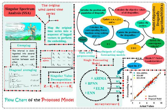
Figure 1.
Flow chart of the developed model.
2.3.1. Data Preprocessing
As noisy data result in poor accuracy, the SSA technique was used to remove fluctuating components and retain the valid information in original wind speed sequences. The original data were decomposed into some IMFs, from which the volatile components were removed and the remainder were reconstructed for effective wind speed forecasting.
2.3.2. Hybrid Models Forecasting
To consider the linear and nonlinear components of short-term wind speed sequences, a classical statistical method (ARIMA) and three effective neural networks, BPNN, ELM, and Elman neural network (ENN), were used to form the basic forecasting model of our system. After integrating these models with the data preprocessing method, hybrid models SSA-ARIMA, SSA-BPNN, SSA-ELM, and SSA-ENN were established to forecast short-term wind speed.
2.3.3. Proposed Combined Forecasting Strategy
In this stage, a weight selection method relying on the MODA was used to find the optimal weight of hybrid strategies, which is crucial for improving forecasting precision and steadiness simultaneously. The data for the last three days in the training set were used to determine the weight coefficient to integrate the hybrid strategies. During the operation of the algorithm, the process is terminated when the iterations number reaches the maximum or the fitness function reaches the minimum. The forecasting results were obtained by combining these hybrid models using the optimized weight coefficients.
2.3.4. Rolling Forecasting
Rolling forecasting mechanism is adopted in our paper, that is, according to the results of trial and error, the input datasets are {x(t − 5), x(t − 4), x(t − 3), x(t − 2), x(t − 1)} and the output datasets is {x(t)}, x represents wind speed time series, and the input and output sets change with the change of t. To assess the forecasting ability of the developed strategy, both one-step and multi-step forecasting are used in our paper. Similarly, three-step ahead forecasting can be determined as follows: the input datasets are {x(t − 5), x(t − 4), x(t − 3), x(t − 2), x(t − 1)} and the output datasets are {x(t + 2)} [41]. A more detailed introduction of rolling forecasting mechanism is also presented in Figure 2.
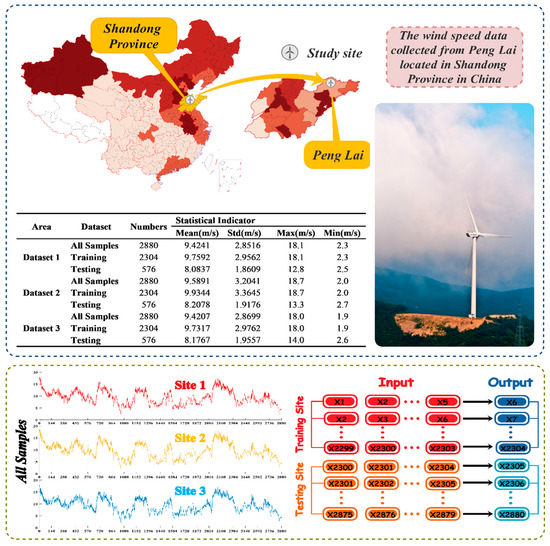
Figure 2.
Observation sites of wind farms and data information.
3. Experimentation Setup
In this section, the setup of our three experiments are introduced, including data selection, performance evaluation criterion, and operating environment.
3.1. Datasets Selection
Raw wind speed data were chosen from four observation points on the Shandong Peninsula in China. Due to its long coastline, Shandong has adequate wind energy resources. All observation sites were located in mountainous and hilly regions with the altitude ranging from 100 m to 240 m above sea level. Generally, the rated power of the wind power generators is 1500 KW, and the height of measurement is 70 m. The time interval in our datasets is 10 min, for a total of 144 records per day.
We chose three datasets as the study cases, with each dataset containing 2880 records with a time span of 1–20 January 2011. The ratio of training set to testing set was 4:1, which included 2304 training samples and 576 testing samples in each group. A rolling forecasting mechanism was applied to one-step and multi-step forecasting to ultimately obtain the forecast of the sixth period based on the first five real time series. The data structure of our proposed model, the research sites, and several statistical indicators of raw wind speed series are provided in Figure 2.
3.2. Performance Evaluation Criteria
Many error indicators have been used in past research; however, no specific standard exists for model evaluation [42]. Thus, multiple evaluation criteria are usually used to compare the developed model and other models with regard to forecasting capacity [43]. In our study, four widely-used error criteria—mean absolute error (MAE), root mean square error (RMSE), mean absolute percent error (MAPE), and sum of squared errors (SSE)—were used as assessment indicators of forecasting performance, whose definitions and equations are listed in Table 1. It must be noted that the measure unit of MAPE in our paper is %.

Table 1.
Performance of assessment criteria.
3.3. Operating Environment
Our experiments were conducted using the Windows 7 professional operating system (Microsoft, Redmond, WA, USA). We used Matlab2016a (MathWorks, Natick, MA, USA) to operate the developed model. The detailed hardware information is: Intel (R) Core i5-4590 3.30 GHz CPU, and 8 GB RAM (Intel Corporation, Santa Clara, CA, USA).
4. Three Experiments and Relative Analysis
In this section, numerical experiments and the corresponding forecasting results are compared and analyzed in detail to provide evidence for the superior forecasting capacity of our developed combined strategy. The experiment setup and results are presented below.
4.1. Experimental Setup
Using actual wind speed time series, we performed three experiments to compare the forecasting ability of the proposed model and other comparable models. Experiment 1 compared the accuracy of our combined model with that of four hybrid models. Experiment 2 compared the differences in the forecasting accuracy of our proposed combined model with other combined models using various data preprocessing technologies. Experiment 3 compared our combined model with four benchmark models to investigate the differences in forecasting capacities. The one-step, two-step, and three-step ahead forecasting capability of the different models were analyzed using the four calculated error criteria. The smaller the value of the error criteria, the better the forecasting performance.
Appropriate parameters are crucial for enhancing wind speed forecasting accuracy and may affect the quality of forecasting results to a certain extent. In our study, the parameters contained in the different models and the different experiments were selected by referring the literature and the actual status of this article to provide useful reference for practical research in the future.
To compare the forecasts of the developed strategy with those of four hybrid strategies without MODA optimization, we conducted Experiment 1. The SSA parameter setting in hybrid strategies is identical to that of the proposed combined strategy, with the specific parameters listed in Table 2. In the rolling forecasting mechanism, the rolling number was 5 and the training-to-testing ratio in all forecasting strategies was set to 3:1.
Table 2.
Parameters in experiment 1.
Experiment 2 was performed to confirm that the forecasting performance of the combined strategy with SSA is superior to those of the other methods using other data preprocessing tools, such as EMD, CEEMD, and wavelet domain de-noising (WDD). In CEEMD, the ratio of the standard deviation of the added noise to the sequences was 0.05 and the realization values and maximum sifting iterations were set to 50 and 500, respectively. The decomposition layer number in WDD was set to 9. For the SSA used in our combined model, the window length and the principal component decomposition number were set to 48 and 20, respectively.
Experiment 3 compared the developed model and four widely-used benchmark models—ARIMA, BPNN, ELM, and ENN—in terms of forecasting performance. Without loss of generality, statistical models and artificial intelligence were considered to show that the forecasting capability far surpasses that of all individual models.
4.2. Experiment 1: Comparison with SSA-Based Hybrid Strategies
The parameters involved in our combined model are provided in Table 2. Based on four error indicators from one- to multi-step forecasting, the proposed combined strategy was confirmed to be the most accurate among the examined models. The comparison results are shown in Table 3, where bold elements indicate the best forecasting performance.
Table 3.
Evaluation metrics comparison of proposed model with relative hybrid models.
For Site 1, the developed strategy produced the best forecasting results in one- and multi-step forecasting with MAPE values of 2.209%, 2.935%, and 3.221% from one-step to three-step, respectively. The other three evaluation criteria obtained for the developed model are also the lowest among all compared models. The differences in the models at Site 1 are provided in Figure 3.
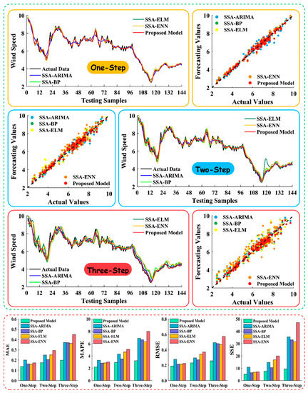
Figure 3.
Comparison of experiment 1 results in site 1.
For Site 2, we forecasted the trend in wind speed using the developed combined model as the MAE, MAPE, RMSE, and SSE results for our combined strategy are superior to those of the other strategies. For instance, the MAPE value of our proposed model is 2.352% and the corresponding MAE, RMSE, and SSE values are 0.145, 0.193, and 5.371, respectively, for one-step forecasting.
For Site 3, the SSA-MODA-based combined model performed the best with a 2.804% MAPE in one-step, 3.193% MAPE in two-step, and 3.588% MAPE in three-step forecasting. Compared with the other hybrid models that improve prediction accuracy to a certain extent, the SSA-MODA-based model is superior.
Remark 1.
We have two main findings here: the prediction of our proposed model is the most accurate, and as the number of forecasting steps increases, the variation in the evaluation criteria in the proposed model from one-step to three-step is minimal, which means the developed strategy provides the best forecasting precision and stability.
4.3. Experiment 2: Comparison of Different Combined Strategies Based on Four Data Preprocessing Technologies
The purpose of experiment 2 was to compare the developed combined model using SSA technology with other combined models employing different data preprocessing technologies. The parameters involved in every method are listed in Table 4 and Table 5, and provide the comparative results for the three sites. The combined models based on EMD, CEEMD, and WDD technology are labeled as EMD-C-Model, CEEMD-C-Model, and WDD-C-Model, respectively.
Table 4.
Parameters in experiment 2.
Table 5.
Comparison of the evaluation metrics for the proposed strategy with models using different data pretreatment technologies.
For Site 1, the proposed combined strategy produced the best forecasting results for all assessment metrics, whereas the others also produced good forecasting results with MAPE values lower than 6%.
For Site 2, the proposed combined strategy also performed better than methods based on other data pretreatment techniques, indicated by MAPE values of 2.352%, 2.966%, and 3.243% for one- to three-step forecasting, respectively. Correspondingly, EMD-C-Model has the worst forecasting accuracy which increases 1.562%, 2.223%, and 2.864%, respectively, relative to SSA based combined model. The comparison results of our SSA-based forecasting strategy and EMD-C-Model, CEEMD-C-Model, and WDD-C-Model are shown in Figure 4.
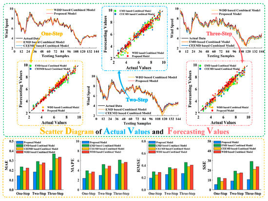
Figure 4.
Comparison results of experiment 2 at site 2.
For Site 3, the SSA-based combined model produced more accurate and effective forecasting compared with the other combined strategies with MAPE value of 2.804% for one-step forecasting. In contrast, the CEEMD-C-Model, WDD-C-Model, and EMD-C-Model had MAPE values of 3.290%, 3.736%, and 4.011%, respectively, which are inferior to our developed combined model.
Remark 2.
We concluded that using the SSA-based forecasting system would be preferable over forecasting systems using other data pretreatment techniques because the MAPE values of the developed strategy, with average MAPE values of 2.789%, 2.854%, and 3.195% for Sites 1 to 3, respectively, are the lowest compared to the other selected models.
4.4. Experiment 3: Comparison with Several Benchmark Strategies
Table 6 and Table 7 present the parameters of the algorithms and compare the results of the developed combined model and several individual models, to demonstrate the forecasting improvement of the developed SSA-MODA combined model.
Table 6.
Parameters in experiment 3.
Table 7.
Comparison of the evaluation metrics of the proposed model with benchmark models.
For Site 1, the proposed combined strategy exceeds the four benchmark strategies in one- and multi-step forecasting. With the increase in prediction steps, the MAPE values of individual models increase significantly, while the values in the proposed model remain stable and fluctuate around two and three. This was also observed for Sites 2 and 3, where the proposed model demonstrated an advantage over the other models.
Taking Site 3 as an example, the MAPE values of our proposed technique are 2.804%, 3.193%, and 3.588% for one- to three-step prediction, followed by the ELM model with MAPE values of 6.176%, 9.031%, and 10.861%, respectively. The ARIMA model produced the largest MAPE values of 7.100%, 9.869%, and 11.871%, respectively. Thus, our developed strategy enhances 3.372%, 5.838%, and 7.273% compared with ELM, and 4.296%, 6.676%, and 8.283% compared with ARIMA from one- to three-step forecasting, respectively. The results of the comparison between the proposed model and the four benchmark models at Site 3 are provided in Figure 5.
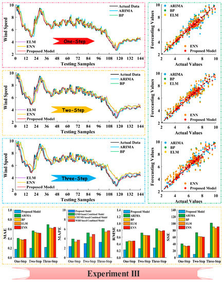
Figure 5.
Comparison of results of experiment 3 at site 3.
Remark 3.
The developed combined model significantly improves forecasting accuracy compared with the benchmark models, as proven by the lower-value evaluation criteria for our proposed model. The MAE, MAPE, RMSE, and SSE values of individual methods are approximate and increase markedly with increasing forecasting steps.
5. Discussion
In this section, seven aspects are discussed to support the forecasting capacity of our proposed combined strategy: forecasting significance, forecasting effectiveness, the degree of improvement, sensitivity analysis, the performance for MODA optimization algorithm, the application of our model in day-ahead forecasts, and the practical application in power system.
5.1. Forecasting Significance: Diebold–Mariano Test
To investigate the differences in forecasting capability between the proposed strategy and the other methods, a typical statistical test, the Diebold–Mariano (DM) test [44] was conducted. The theory of this test is outlined below.
Firstly, formulate original hypothesis H0 and alternative hypothesis H1. H0 signifies that the forecasting capability of the developed strategy is analogous to that of the compared model, whereas H1 is the opposite. The specific hypothetical formulas are written as follows:
where L is the loss function of forecasting errors; , j = 1, 2 represents the forecasting errors of the other methods.
Subsequently, set the DM statistic, which is expressed as
where S2 is the estimated variance of .
Given a certain level of significance , the calculated statistics were compared with critical value . If the DM statistic was not included in the interval , H0 was rejected, which means that significant differences exist between our developed combined strategy and the compared model; otherwise, H0 is accepted.
Table 8 lists the mean DM values from one- to multi-step forecasting. The proposed model is markedly different from individual models including ARIMA, BPNN, ELM, and ENN at the 1% significance level. Although the DM values obtained from the comparison between the developed strategy and SSA-based hybrid methods are not significant as that obtained from the comparison with individual models, the SSA-based combined model has a better forecasting ability compared with four hybrid models at the 10% significance level. Finally, when comparing the developed model with models applying different data pretreatment technologies, the degree of the difference was huge because the DM statistics from one- to three-step all surpass the critical values at the 1% significance level, which signifies a 99% possibility that H1 will be accepted.
Table 8.
Diebold–Mariano (DM) test results for the developed model and comparison models.
The DM statistics show that the developed combined strategy is distinguished from the benchmark models, SSA-based hybrid methods, as well as combined forecasting models using different data preprocessing methods. Thus, the developed combined model should be employed in practical wind speed forecasting.
5.2. Forecasting Effectiveness of the Developed Strategy
In this subsection, the forecasting effectiveness is examined to determine whether the developed strategy is superior to other compared models [45]. As for forecasting effectiveness, both first- and second-order are available, where first-order forecasting effectiveness is relative to the expected values of forecasting precision sequences and second-order is relative to the distinction between standard deviation and expected value of the forecasting precision sequences. The forecasting ability increased with increasing forecasting effectiveness. Table 9 lists the computed forecasting effectiveness values of all forecasting models examined in our study, which shows that our proposed model forecasts better than all the other models at the selected three sites. The forecasting effectiveness values obtained from the proposed model were the highest among all models, with first-order values of 0.974, 0.973, and 0.969 and second-order values of 0.952, 0.951, and 0.946 for Sites 1, 2, and 3, respectively. The forecasting effectiveness values obtained for SSA-based hybrid models were similar to those calculated for models based on different data preprocessing techniques. The forecasting effectiveness values for the benchmark models were the lowest.
Table 9.
Forecasting effectiveness of our proposed combined strategy.
Thus, we conclude that the SSA-MODA combined model has potential to improve wind speed forecasting accuracy compared with the other selected models. Both the first- and second-order forecasting effectiveness values of the developed strategy are satisfactory, indicating that the proposed model can simultaneously improve forecasting accuracy and stability.
5.3. Improvements Percentage Relative to Other Involved Models
Based on the previous analysis, the proposed combined strategy exceeds the other strategies in terms of forecasting accuracy improvement. To further discuss and evaluate the degree improvement in forecasting when comparing a selected model with the proposed model, we examined four additional metrics: PMAE, PMAPE, PRMSE, and PSSE [46]. The four metrics are briefly described in Table 10; Table 11 provides the improvement percentages of the developed strategy over the selected methods. According to the definition the larger the improvement percentage values, the better the forecasting accuracy of our developed model relative to the selected models. From our analysis of the results in Table 11:
Table 10.
Brief definition of four metrics.
Table 11.
Improvement percentages of the proposed model relative to selected models.
- (1)
- The developed combined model markedly increases wind speed forecasting accuracy relative to the selected models, with improvement percentages from more than 20% up to 80%.
- (2)
- When the proposed model was compared with four individual models, the PMAE, PMAPE, PRMSE, and PSSE values obtained for the ARIMA model are the highest. Similar to previous research, the improvement percentages for the majority of metrics for the SSA-based hybrid model and the combined models using other data preprocessing methods are similar, which vary from 30% to 50%.
- (3)
- These results reveal that the combination of a data pretreatment technique and an optimization algorithm significantly improves forecasting accuracy in our combined model; only adding a data pretreatment technique or only using hybrid model are insufficient to improving forecast precision and stability simultaneously for short-term wind speed forecasting.
5.4. Sensitivity Analysis
To further study how varying the data pretreatment technique parameters and multi-objective optimization algorithm affects the performance of the proposed model, sensitivity analysis was conducted. In the calculation, we used the standard deviation of each error criterion as the novel assessment metric for sensitivity (SMAE, SMAPE, SRMSE, and SSSE) [47]. The robustness decreases with increasing novel assessment metrics. Table 12 provides the calculated results obtained by altering one parameter of SSA or MODA with the remaining parameters unchanged. The relevant parameters in SSA are window length and principal component decomposition number, whereas the parameters in MODA are dragonfly number, iteration number, and archive size.
Table 12.
Results of sensitivity indicators obtained from SSA and MODA.
Without loss of generality, the analysis was divided into two parts: the parameters variation in SSA and in MODA. The window lengths considered in SSA were 32, 40, 48, 56, and 64, and the principal component decomposition numbers used were 10, 15, 20, 25, and 30. In the analysis of MODA parameter variation, the assigned dragonfly numbers were 20, 40, 60, 80, and 100; the iteration numbers were 50, 100, 150, 200, and 250; and the archive size was set to 200, 300, 400, 500, and 600. Our analysis of Table 12 provided the following:
- (1)
- When the parameters in SSA were changed, the SMAE, SMAPE, SRMSE, and SSSE values changed within acceptable limits. For instance, in one-step forecasting at Site 1, the SMAE, SMAPE, and SRMSE, SSSE values for window length were 0.004, 0.085, 0.003, and 0.177, respectively, and the principal component decomposition number values were 0.009, 0.154, 0.008, and 0.457, respectively, which are small and similar to the values obtained for Sites 2 and 3. In other words, the forecasting results of the proposed strategy are not considerably affected by parameter variation in SSA.
- (2)
- With altering the MODA parameter, the assessment criteria for sensitivity changes within acceptable limits. The results reveal that changing the optimization parameters has a minimal influence on the forecasting results of our developed model, which further verifies the stability of the proposed model.
- (3)
- The SMAE, SMAPE, SRMSE, and SSSE values in two- and three-step forecasting are larger than in one-step forecasting, revealing that the forecasting robustness declines with parameters variation when increasing the forecasting steps. We found that in two-step forecasting at Site 1, the SSSE values of the five parameters were abnormal and far larger than the other assessment metrics, which can be attributed to the randomness and volatility of the selected dataset. Therefore, choosing suitable parameters in multi-step forecasting is crucial as parameters variation impacts the stability of wind speed forecasting to some extent.
5.5. Comparison in Terms of Optimization Algorithm Performance
To further verify the superiority of the MODA over other optimization algorithms in terms of short-term wind speed forecasting, three combined models based on three good performing optimization algorithms, including Elitist Nondominated Sorting Genetic Algorithm (NSGA II) [48], multi-objective particle swarm optimization (MOPSO) [49], and multi-objective ant lion optimization (MOALO) [50], were used to compare with the developed model with MODA algorithm. The comparative results are established in Table 13, based on which we can conduct the following discussions:
Table 13.
Comparison of the evaluation metrics for the proposed strategy with models using different optimization algorithms.
- (1)
- Regardless of the forecasting steps and observation sites, the employed MODA was always superior to NSGA II, MOPSO, and MOALO indicated by the lower MAE, MAPE, RMSE, and SSE values. For example, the mean MAPE values of the developed model are 2.789%, 2.854%, and 3.195% from Site 1 to Site 3, respectively, whereas the mean MAPE values of combined model using NSGA II algorithm (5.439%, 5.184%, 5.186%, respectively), combined model using MOPSO algorithm (4.735%, 4.605%, 4.574%, respectively), and combined model using the MOALO algorithm (4.151%, 4.373%, 4.313%, respectively) are obviously inferior to the proposed model based on MODA algorithm. Thus, the MODA algorithm can provide better forecasting results relative to NSGA II, MOPSO, and MOALO algorithm in combined short-term wind speed forecasting system.
- (2)
- From another perspective, with the increase of forecasting steps, the evaluation criteria values of the proposed model changes in a much smaller range compared with other comparative models, which reveals that the developed model with MODA algorithm can provide more stable and robust forecasting performance. In Site 1, the MAPE values of the proposed model from one-step to three-step forecasting are 2.209%, 2.935%, and 3.221%, and in the same condition, the corresponding values obtained from the MOALO based combined model whose forecasting capacity is second only to the MODA algorithm are 3.046%, 4.203%, and 5.203%, respectively. Thus, when the forecasting steps increase, the MAPE values of MOALO based combined model increase rapidly compared with the proposed MODA based combined model, which also applies to NAGA II and MOPSO algorithm. Ultimately, we can conclude that MODA is a powerful tool for solving multi-objective optimization issues in our work, significantly improving forecasting accuracy and stability.
5.6. The Forecasting Performance Verify of Our Model with Longer Testing Set
In order to further test the long-term prediction ability of our proposed model, we expanded the original data set to 5760 records with a time span of 1 January to 9 February 2011. The ratio of training set to testing set was still 4:1, indicating that 4608 training samples and 1152 testing samples in each dataset and the observation sites are the same as that in the previous experiments. Accordingly, the forecasting horizon of the combined model reaches 288 periods, that is, two days. If the prediction performance of our proposed model is good in this case, it will prove that after one training, our proposed model can maintain a high prediction accuracy and avoid training the proposed model again when rolling the prediction of future wind speed of 288 periods. SSA-BP, CEEMD-C-model, ELM, and MOALO-C-model are adopted in this discussion as comparative models due to their relatively superior forecasting ability in previous experiments and discussion. The comparison results for the proposed model based on the testing set with two-day length and some good performing models based on the testing set with two-day length are presented in Table 14, where CEEMD-C-model and MOALO-C-model represent the CEEMD-MODA based combined model and SSA-MOALO based combined model. From the table, we can conduct that the developed model can always provide accurate and stable forecasting when the testing set length becomes two days. The detailed analysis in terms of the comparative results are presented in the following:
Table 14.
Comparison of forecasting evaluation metrics based on the testing set with two days length for the proposed strategy with some good performing models.
- (1)
- With longer duration of continuous prediction, the proposed combined model can achieve satisfactory forecasting performance in the selected observation sites whether in one-step forecasting or multi-step forecasting. For example, the mean MAPE of the proposed model in Site 1 is 3.133% and corresponding mean MAE, RMSE, and SSE values are 0.191, 0.253, and 8.294, which improve to a great extent compared with ELM forecasting model whose forecasting capacity is the worst among all selected models. Similar to the forecasting results based on the testing set with one-day length, the proposed model can always provide more stable forecasting results because the evaluation criteria values increase slightly with the increase of forecasting steps, whereas the values in other models increase to a great extent.
- (2)
- Compared with the forecasting results based on the testing set with one-day length, the simulation results based on the testing set with two-day length (intra-day and the next day’s forecasting) display slightly higher errors, either one step or multi-step. This is understandable because more uncertain information is contained in forecasting process when the forecasting length increases. For example, the mean MAPE values of the proposed model in this section are 3.133%, 3.282%, and 3.604%, respectively and the corresponding values in the forecasting based on the testing set with one-day length are 2.789%, 2.854%, and 3.195% from Site 1 to Site 3, respectively. It does not mean that our developed model is invalid for wind speed forecasting based on the testing set with a longer length because the MAE, MAPE, RMSE, and SSE values are all better than the compared models with more accurate and stable forecasting performance. Thus, it is credible and reliable that the developed model can achieve great forecasting performance whether based on the testing set with one-day length or two-day length.
5.7. Pragmatic Applications in Power Systems
Accurate wind speed forecasting is a prerequisite to improve the stability of wind power systems and the efficiency of wind power generation [51,52]. As an improvement to the existing wind power systems, the developed wind speed prediction strategy, with the target of improving prediction accuracy and stability, shows the ability to minimize the risks of wind power generation due to wind variation and achieve real-time forecasting in terms of wind power generation scheduling and safe operation [53]. The contributions of an effective wind speed forecasting system to power systems are listed below:
- Optimizing the potential wind energy in every wind farm is important for maintaining the upper limit of wind energy output. As wind energy is proportional to the cube of wind speed, precisely predicting wind speed is critical so that the wind energy capacity can be determined, and smart grids can be effectively planned by decision makers [54].
- With wind speed forecasting, decisions regarding the operation and administration of wind turbines can be credibly made. To ensure the largest output of wind energy, managers can alter the wind turbine potential without delay according to the predicted wind. Once the wind turbine capacity is under the forecasted wind speed, the output can be closed to prevent breakdown and minimize operation costs.
- The scheduling and management of power systems, to a large extent, rely on wind speed forecasting. We must consider the balance between power demand and supply to satisfy demand and ensure sustainable energy development. Excess power supply poses a problem in practical applications, which may result in supply quality degradation, power system insecurity, and operational cost increases [55]. Thus, it is imperative to formulate more exact and stable wind speed forecasting models to assist decision makers to make timely decisions so that these problems can be effectively addressed.
6. Conclusions
Short-term wind speed forecasting, an important tool in wind energy research and practical applications, has been growing in popularity, mostly due to its importance in the scheduling and operation of power grids [56]. However, wind speed time series are fluctuating and stochastic, which creates challenges for wind speed forecasting and generation. Anticipating this constraint is important because higher uncertainty requires more comprehensive forecasting models to meet specified accuracy and stability objectives [57]. In this study, we developed a combined strategy that effectively integrates data preprocessing technology and an optimization algorithm and significantly improves wind speed forecasting accuracy and stability. To overcome the passive impacts of high-frequency noise on forecasting performance, an effective de-noising method was firstly applied to decompose raw wind speed sequences and retain the fundamental characteristics of wind speed data. Then, a typical statistical model, ARIMA, and three classical neural networks, BPNN, ELM, and ENN, were used as wind speed forecasting system benchmarks. To combine these forecasting models, MODA was successfully used to confirm the optimal weight coefficient of our developed SSA-MODA system. Based on the above processes and actual wind speed sequences, three numerical experiments, four evaluation criteria, and seven discussions were conducted to verify the accuracy and stability of our developed model. In experiment 1, the MAPE values of one-step forecasting obtained at Sites 1 to 3 in our developed strategy were 2.209%, 2.935%, and 3.221%, respectively, whereas the lowest MAPE values in the compared models were 2.836%, 3.506%, and 6.310%, respectively, which are larger than in the developed model. In Experiments 2 and 3, regardless of the forecasting step or the observation site, the proposed combined strategy was always superior to all the selected methods because the performance metrics were the lowest and fluctuated over a small range, indicating that the proposed strategy accurately and stably predicts short-term wind speed. Moreover, in the discussions, we have verified the forecasting significance and forecasting effectiveness of our developed model and further proved that our proposed model can provide accurate and stable wind speed forecasting performance. To verify the superiority of MODA, we conduct a comparison among MODA, NAGA II, MOPSO, and MOALO, and the results indicate that the MODA is a helpful choice for short-term wind speed forecasting in our work. Besides, the developed model is used to intra-day and next day forecasting and the simulation results have testified the effectiveness of our developed model in both intra-day and next day forecasting, which can help wind producers bid their offers in day-ahead schedule. Ultimately, the practical applications of the developed model in power system are illuminated in detail to verify the practical value of the developed model. Overall, the developed model significantly increases short-term wind speed forecasting accuracy and stability, providing a reference for smart grid planning.
The main limitation of this research is that only power systems including wind farms were considered, whereas other fields including stock price forecasting were not included. Recommendations for improvements in our work in the future include:
- (1)
- Applying more effective data pretreatment techniques to handle the stochastic and fluctuating wind speed data to increase the forecasting accuracy.
- (2)
- Improving existing optimization algorithms to enhance the global search ability and convergence speed and further improving optimization performance and forecasting accuracy of combined models.
- (3)
- Developing new neural network models and statistic methods to grasp the characteristic of wind speed series and constructing fundamental forecasting models.
Author Contributions
Software, Z.L.; Supervision, J.W.; Writing—original draft, Y.D.; Writing—review and editing, L.Z. All authors have read and agreed to the published version of the manuscript.
Funding
This research is supported by the National Natural Science Foundation of China (Grant No. 71761016), Natural Science Foundation of Jiangxi (Grant No. 20171BAA218001), Scientific Research Fund of Jiangxi Provincial Education Department (Grant No. GJJ180287), Postdoctoral Foundation of Jiangxi Province (Grant No. 2018KY08) and Humanities and Social Sciences Foundation of Jiangxi University (Grant No. TJ19202).
Conflicts of Interest
The authors declare no conflict of interest.
Abbreviations
| FL | fuzzy logic |
| KF | Kalman filtering |
| ENN | elman neural network |
| ANN | artificial neural network |
| RMSE | root mean square error |
| IMFs | intrinsic mode functions |
| NWP | numerical weather prediction |
| BP | back propagation neural network |
| EEMD | ensemble empirical mode decomposition |
| MOALO | multi-objective ant lion optimization |
| ARIMA | autoregressive integrated moving average model |
| ARFIMA | autoregressive fractional integrated moving average |
| CEEMD | complete ensemble empirical mode decomposition |
| MODA | multi-objective dragonfly optimization algorithm |
| MOGWO | multi-objective grey wolf optimization algorithm |
| MC | Markov chain |
| CS | cuckoo search |
| MAE | mean absolute error |
| SSE | error sum of square |
| WNN | wavelet neural network |
| DM Test | Diebold Mariano test |
| ELM | extreme learning machine |
| WDD | wavelet domain de-noising |
| SSA | singular spectrum analysis |
| EMD | empirical model decomposition |
| MAPE | mean absolute percentage error |
| DA | dragonfly optimization algorithm |
| MOPSO | multi-objective particle swarm optimization |
| NSGA II | Elitist Nondominated Sorting Genetic Algorithm |
References
- Li, R.; Jin, Y. A wind speed interval prediction system based on multi-objective optimization for machine learning method. Appl. Energy 2018, 228, 2207–2220. [Google Scholar] [CrossRef]
- Salcedo-Sanz, S.; Pérez-Bellido, Á.M.; Ortiz-García, E.G.; Portilla-Figueras, A.; Prieto, L.; Correoso, F. Accurate short-term wind speed forecasting by exploiting diversity in input data using banks of artificial neural networks. Neurocomputing 2009, 72, 1336–1341. [Google Scholar] [CrossRef]
- Data on Global Onshore and Offshore Wind Power in 2018. Available online: http://news.bjx.com.cn/html/20190516/980725.shtml (accessed on 30 June 2019).
- Calif, R.; Schmitt, F. Multiscaling and joint multiscaling of the atmospheric wind speed and the aggrgate power output from a wind farm. Nonlinear Processes Geophys. 2014, 21, 379–392. [Google Scholar] [CrossRef]
- Jiang, P.; Liu, Z. Variable weights combined model based on multi-objective optimization for short-term wind speed forecasting. Appl. Soft Comput. 2019, 82, 105587. [Google Scholar] [CrossRef]
- Zhou, Q.; Wang, C.; Zhang, G. Hybrid forecasting system based on an optimal model selection strategy for different wind speed forecasting problems. Appl. Energy 2019, 250, 1559–1580. [Google Scholar] [CrossRef]
- Bo, H.; Niu, X.; Wang, J. Wind Speed Forecasting System Based on the Variational Mode Decomposition Strategy and Immune Selection Multi-Objective Dragonfly Optimization Algorithm. IEEE Access 2019, 7, 178063–178081. [Google Scholar] [CrossRef]
- Zhao, X.; Liu, J.; Yu, D.; Chang, J. One-day-ahead probabilistic wind speed forecast based on optimized numerical weather prediction data. Energy Convers. Manag. 2018, 164, 560–569. [Google Scholar] [CrossRef]
- Alessandrini, S.; Sperati, S.; Pinson, P. A comparison between the ECMWF and COSMO Ensemble Prediction Systems applied to short-term wind power forecasting on real data. Appl. Energy 2013, 107, 271–275. [Google Scholar] [CrossRef]
- Sile, T.; Bekere, L.; Cepite-Frisfelde, D.; Sennikovs, J.; Bethers, U. Verification of numerical weather prediction model results for energy applications in Latvia. Energy Procedia 2014, 59, 213–220. [Google Scholar] [CrossRef]
- Liu, H.; Tian, H.-Q.; Chen, C.; Li, Y. A hybrid statistical method to predict wind speed and wind power. Renew. Energy 2010, 35, 1857–1861. [Google Scholar] [CrossRef]
- Shukur, O.B.; Lee, M.H. Daily wind speed forecasting through hybrid KF-ANN model based on ARIMA. Renew. Energy 2015, 76, 637–647. [Google Scholar] [CrossRef]
- Yuan, X.; Tan, Q.; Lei, X.; Yuan, Y.; Wu, X. Wind power prediction using hybrid autoregressive fractionally integrated moving average and least square support vector machine. Energy 2017, 129, 122–125. [Google Scholar] [CrossRef]
- Jiang, H. Model forecasting based on two-stage feature selection procedure using orthogonal greedy algorithm. Appl. Soft Comput. 2018, 63, 10–15. [Google Scholar] [CrossRef]
- Du, P.; Wang, J.; Yang, W.; Niu, T. A novel hybrid model for short-term wind power forecasting. Appl. Soft Comput. J. 2019, 80, 93–106. [Google Scholar] [CrossRef]
- Jiang, H.; Dong, Y. Structural regularization in quadratic logistic regression model. Knowl.-Based Syst. 2019, 163, 842–857. [Google Scholar] [CrossRef]
- Wang, R.; Li, J.; Wang, J.; Gao, C. Research and Application of a Hybrid Wind Energy Forecasting System Based on Data Processing and an Optimized Extreme Learning Machine. Energies 2018, 11, 1712. [Google Scholar] [CrossRef]
- Hao, Y.; Tian, C.; Wu, C. Modelling of carbon price in two real carbon trading markets. J. Clean. Prod. 2020, 244, 118556. [Google Scholar] [CrossRef]
- Tian, C.; Hao, Y. Point and interval forecasting for carbon price based on an improved analysis-forecast system. Appl. Math. Model. 2019. [Google Scholar] [CrossRef]
- Wang, J.; Wu, C.; Niu, T. A Novel System for Wind Speed Forecasting Based on Multi-Objective Optimization and Echo State Network. Sustainability 2019, 11, 526. [Google Scholar] [CrossRef]
- Pourmousavi Kani, S.A.; Ardehali, M.M. Very short-term wind speed prediction: A new artificial neural network–Markov chain model. Energy Convers. Manag. 2011, 52, 738–745. [Google Scholar] [CrossRef]
- Yang, W.; Wang, J.; Lu, H.; Niu, T.; Du, P. Hybrid wind energy forecasting and analysis system based on divide and conquer scheme: A case study in China. J. Clean. Prod. 2019, 222, 942–959. [Google Scholar] [CrossRef]
- Xiao, L.; Shao, W.; Yu, M.; Ma, J.; Jin, C. Research and application of a hybrid wavelet neural network model with the improved cuckoo search algorithm for electrical power system forecasting. Appl. Energy 2017, 198, 203–205. [Google Scholar] [CrossRef]
- Zhao, X.; Wang, C.; Su, J.; Wang, J. Research and application based on the swarm intelligence algorithm and artificial intelligence for wind farm decision system. Renew. Energy 2019, 134, 681–697. [Google Scholar] [CrossRef]
- Wang, J.; Niu, T.; Lu, H.; Yang, W.; Du, P. A Novel Framework of Reservoir Computing for Deterministic and Probabilistic Wind Power Forecasting. IEEE Trans. Sustain. Energy 2019. [Google Scholar] [CrossRef]
- Wu, C.; Wang, J.; Chen, X.; Du, P.; Yang, W. A Novel Hybrid System Based on Multi-objective Optimization for Wind Speed Forecasting. Renew. Energy 2019. [Google Scholar] [CrossRef]
- Liu, H.; Chen, C.; Tian, H.Q.; Li, Y.F. A hybrid model for wind speed prediction using empirical mode decomposition and artificial neural networks. Renew. Energy 2012, 48, 545–556. [Google Scholar] [CrossRef]
- Bates, J.M.; Granger, C.W.J. The Combination of Forecasts. J. Oper. Res. Soc. 1969, 20, 451–468. [Google Scholar] [CrossRef]
- Niu, T.; Wang, J.; Lu, H.; Du, P. Uncertainty modeling for chaotic time series based on optimal multi-input multi-output architecture: Application to offshore wind speed. Energy Convers. Manag. 2018, 156, 597–617. [Google Scholar] [CrossRef]
- Zhang, S.; Wang, J.; Guo, Z. Research on combined model based on multi-objective optimization and application in time series forecast. Soft Comput. 2019, 23, 11493–11521. [Google Scholar] [CrossRef]
- Hao, Y.; Tian, C. The study and application of a novel hybrid system for air quality early-warning. Appl. Soft Comput. 2019, 74, 729–746. [Google Scholar] [CrossRef]
- Jiang, H. Sparse estimation based on square root nonconvex optimization in high-dimensional data. Neurocomputing 2018, 282, 122–125. [Google Scholar] [CrossRef]
- Niu, X.; Wang, J. A combined model based on data preprocessing strategy and multi-objective optimization algorithm for short-term wind speed forecasting. Appl. Energy 2019, 241, 519–539. [Google Scholar] [CrossRef]
- Li, H.; Wang, J.; Lu, H.; Guo, Z. Research and application of a combined model based on variable weight for short term wind speed forecasting. Renew. Energy 2018, 116, 669–684. [Google Scholar] [CrossRef]
- Hassani, H.; Ghodsi, Z. A glance at the applications of Singular Spectrum Analysis in gene expression data. Biomol. Detect. Quantif. 2015, 4, 17–21. [Google Scholar] [CrossRef]
- Krishnannair, S.; Aldrich, C.; Jemwa, G.T. Detecting faults in process systems with singular spectrum analysis. Chem. Eng. Res. Des. 2016, 113, 151–155. [Google Scholar] [CrossRef]
- Unnikrishnan, P.; Jothiprakash, V. Daily rainfall forecasting for one year in a single run using Singular Spectrum Analysis. J. Hydrol. 2018, 561, 609–621. [Google Scholar] [CrossRef]
- De Carvalho, M.; Rua, A. Real-time nowcasting the US output gap: Singular spectrum analysis at work. Int. J. Forecast. 2015, 33, 185–198. [Google Scholar] [CrossRef]
- Mirjalili, S. Dragonfly algorithm: A new meta-heuristic optimization technique for solving single-objective, discrete, and multi-objective problems. Neural Comput. Appl. 2015, 27, 1053–1073. [Google Scholar] [CrossRef]
- Li, H.; Wang, J.; Li, R.; Lu, H. Novel analysis–forecast system based on multi-objective optimization for air quality index. J. Clean. Prod. 2019, 208, 1365–1383. [Google Scholar] [CrossRef]
- Yang, W.; Wang, J.; Niu, T.; Du, P. A hybrid forecasting system based on a dual decomposition strategy and multi-objective optimization for electricity price forecasting. Appl. Energy 2019. [Google Scholar] [CrossRef]
- Liu, Z.; Jiang, P.; Zhang, L.; Niu, X. A combined forecasting model for time series: Application to short-term wind speed forecasting. Appl. Energy 2019, 114137. [Google Scholar] [CrossRef]
- Yang, H.; Zhu, Z.; Li, C.; Li, R. A novel combined forecasting system for air pollutants concentration based on fuzzy theory and optimization of aggregation weight. Appl. Soft Comput. 2019, 105972. [Google Scholar] [CrossRef]
- Diebold, F.X.; Mariano, R.S. Comparing predictive accuracy. J. Bus. Econ. Stat. 1995, 13, 253–265. [Google Scholar] [CrossRef]
- Chen, H.; Hou, D. Research on superior combination forecasting model based on forecasting effective measure. J. Univ. Sci. Technol. China 2002, 32, 172–180. [Google Scholar]
- Mi, X.; Liu, H.; Li, Y. Wind speed prediction model using singular spectrum analysis, empirical mode decomposition and convolutional support vector machine. Energy Convers. Manag. 2019, 180, 196–205. [Google Scholar] [CrossRef]
- Wang, J.; Du, P.; Lu, H.; Yang, W.; Niu, T. An improved grey model optimized by multi-objective ant lion optimization algorithm for annual electricity consumption forecasting. Appl. Soft Comput. J. 2018, 72, 321–337. [Google Scholar] [CrossRef]
- Sarshar, J.; Moosapour, S.S.; Joorabian, M. Multi-objective energy management of a micro-grid considering uncertainty in wind power forecasting. Energy 2017. [Google Scholar] [CrossRef]
- He, Z.; Chen, Y.; Shang, Z.; Li, C.; Li, L.; Xu, M. A novel wind speed forecasting model based on moving window and multi-objective particle swarm optimization algorithm. Appl. Math. Model. 2019. [Google Scholar] [CrossRef]
- Du, P.; Wang, J.; Guo, Z.; Yang, W. Research and application of a novel hybrid forecasting system based on multi-objective optimization for wind speed forecasting. Energy Convers. Manag. 2017. [Google Scholar] [CrossRef]
- Zhou, J.; Sun, N.; Jia, B.; Peng, T. A Novel Decomposition-Optimization Model for Short-Term Wind Speed Forecasting. Energies 2018, 11, 1752. [Google Scholar] [CrossRef]
- Iversen, E.B.; Morales, J.M.; Møller, J.K.; Madsen, H. Short-term probabilistic forecasting of wind speed using stochastic differential equations. Int. J. Forecast. 2015, 32, 981–990. [Google Scholar] [CrossRef]
- Sun, N.; Zhou, J.; Chen, L.; Jia, B.; Tayyab, M.; Peng, T. An adaptive dynamic short-term wind speed forecasting model using secondary decomposition and an improved regularized extreme learning machine. Energy 2018. [Google Scholar] [CrossRef]
- Zuluaga, C.D.; Álvarez, M.A.; Giraldo, E. Short-term wind speed prediction based on robust Kalman filtering: An experimental comparison. Appl. Energy 2015. [Google Scholar] [CrossRef]
- Zhang, X.; Wang, J.; Gao, Y. A hybrid short-term electricity price forecasting framework: Cuckoo search-based feature selection with singular spectrum analysis and SVM. Energy Econ. 2019, 81, 899–913. [Google Scholar] [CrossRef]
- Wang, J.; Gao, Y.; Chen, X. A novel hybrid interval prediction approach based on modified lower upper bound estimation in combination with multi-objective salp swarm algorithm for short-term load forecasting. Energies 2018, 11, 1561. [Google Scholar] [CrossRef]
- Zhang, L.; Dong, Y.; Wang, J. Wind Speed Forecasting Using a Two-Stage Forecasting System with an Error Correcting and Nonlinear Ensemble Strategy. IEEE Access 2019, 7, 176000–176023. [Google Scholar] [CrossRef]
© 2019 by the authors. Licensee MDPI, Basel, Switzerland. This article is an open access article distributed under the terms and conditions of the Creative Commons Attribution (CC BY) license (http://creativecommons.org/licenses/by/4.0/).