Fault Diagnosis Method for Hydraulic Directional Valves Integrating PCA and XGBoost

Abstract

A novel fault diagnosis method is proposed, depending on a cloud service, for the typical faults in the hydraulic directional valve. The method, based on the Machine Learning Service (MLS) HUAWEI CLOUD, achieves accurate diagnosis of hydraulic valve faults by combining both the advantages of Principal Component Analysis (PCA) in dimensionality reduction and the eXtreme Gradient Boosting (XGBoost) algorithm. First, to obtain the principal component feature set of the pressure signal, PCA was utilized to reduce the dimension of the measured inlet and outlet pressure signals of the hydraulic directional valve. Second, a machine learning sample was constructed by replacing the original fault set with the principal component feature set. Third, the MLS was employed to create an XGBoost model to diagnose valve faults. Lastly, based on model evaluation indicators such as precision, the recall rate, and the F1 score, a test set was used to compare the XGBoost model with the Classification And Regression Trees (CART) model and the Random Forests (RFs) model, respectively. The research results indicate that the proposed method can effectively identify valve faults in the hydraulic directional valve and have higher fault diagnosis accuracy.

1. Introduction

Hydraulic systems play an important role in a wide variety of industrial applications, such as robotics, manufacturing, aerospace, and engineering machinery. Monitoring the condition of hydraulic equipment can not only effectively improve productivity and reduce maintenance costs and downtime, but also improve the reliability and safety of this equipment in its application [1,2,3]. In particular, the hydraulic valve is the core control component of the hydraulic system, and it is widely used in numerous engineering applications to control the flow and pressure of fluids [4,5,6]. In the hydraulic system, a vibration analysis (VA) is the most popular and efficient condition monitoring technique for rotating systems including the hydraulic pump, electric motor, bearing, and more [7,8,9,10,11,12,13,14,15,16]. However, the working process of the valve core of the hydraulic valve is a reciprocating motion. These VA methods, which have been successfully applied in rotating machinery, will not be suitable for fault diagnosis and a condition monitoring signal analysis of non-rotating machinery, such as the hydraulic valve [17,18,19].

Many studies on fault diagnosis of the hydraulic valve have been conducted by theoretical approaches and test measurements, and certain research results have been obtained. Wu et al. [20] proposed a method for the mechanical fault diagnosis based on complex three-order cumulants. In the experiment regarding the fault diagnosis of the overflow valve, the results show that this method can improve the correction rate of diagnosis. Huang et al. [21] applied the theory of higher-order spectrum to the fault diagnosis of hydraulic valves. Li et al. [22] proposed a fault diagnosis method that involves choosing the fractal characteristic volume of a valve’s displacement signal as a criterion to solve the nonlinear problems in the working process of autopilot hydraulic valves. Raduenz et al. [23] presented the development of a method for condition monitoring and online fault detection on proportional reversing valves. The effectiveness of the method to monitor and detect faults in valves with different sizes and constructive parameters was shown experimentally using five different proportional valves. Vianna et al. [24] presented a method to estimate degradation in a servo valve using an application of the Fading Extended Kalman Filter for system identification. Folmer et al. [25] also presented a data-driven fault detection system for valves, which uses historical process data obtained across company borders to detect faults by comparing standardized flow coefficients determined by DIN IEC 60534-2-1 in physical valve models. Moreover, many challenges emerge in the study of the condition monitoring and fault diagnosis of hydraulic valves. In particular, there are few research results for identifying hydraulic valve faults by pressure signals in the hydraulic system with condition monitoring on an Industrial Internet of Things (IIoT) platform.

Due to the availability of big data technology and data mining methods as well as the emergence of new IIoT platforms and machine learning algorithms, fault diagnosis for hydraulic valves based on big data for hydraulic system with condition monitoring is one of the focuses for this research [26,27,28]. Among them, Principal Component Analysis (PCA) is an effective method for dimensionality reduction in big data analysis. It is a multivariate statistical method, which compresses multiple linearly related variables into a few unrelated variables. PCA was first proposed by Pearson [29] in a study on optimal linear and plane fitting of spatial data. Fisher and Mackenzie [30] believed that PCA was more useful in the system response variance analysis than in system modeling, and they proposed a prototype of the Nonlinear Iterative Partial Least Squares (NIPALS) algorithm. Then, PCA was improved by Hoteling [31] and further developed into a common method widely used in data dimensionality reduction, fault diagnosis, and anomaly detection. For instance, Mohanty et al. [32] developed a new algorithm to identify bearing faults using empirical mode decomposition and principal component analysis (EMD-PCA) based on the average kurtosis technique. It was observed that this proposed combined approach effectively and adaptively identified inner ball faults. Stief et al. [33] proposed a sensor fusion approach to diagnose both electrical and mechanical faults in induction motors based on the combination of a two-stage Bayesian method and PCA. Caggiano [34] also proposed an advanced feature extraction methodology based on PCA. By introducing artificial neural networks to the PCA features, an accurate diagnosis of tool flank wear was achieved, with predicted values being very close to the measured tool wear values. Wang et al. [35] developed a variable selection algorithm based on PCA with multiple selection criteria, which can identify faults in wind turbines, determine the corresponding time and location where the fault occurs, and estimate its severity. Xiao et al. [36] also studied the application of PCA to fault diagnosis in Electro-Hydrostatic Actuators (EHAs). The experimental results demonstrated that PCA can effectively discriminate faults and their characteristics for EHAs, and could be used as an optional data fusion tool for the Prognostics and Health Management (PHM) of EHAs. Riba et al. [37] proposed a very fast, noninvasive, accurate, and easy-to-apply method to discriminate between paperboard samples produced from recovered and virgin fibers. For this method, FTIR spectroscopy was analyzed in combination with feature extraction methods such as PCA, PCA+ canonical variate analysis (CVA), extended canonical variate analysis (ECVA), and the k Nearest Neighbor algorithm (kNN) classifier. The experimental results proved that the proposed scheme allowed for the obtainment of a high classification accuracy with a very fast response.

In addition, the eXtreme Gradient Boosting (XGBoost) algorithm, proposed by Dr. Chen Tianqi in 2014, can automatically utilize the central processing unit (CPU) multi-threaded parallel computing and has the advantages of low computational complexity, fast running speed, and high accuracy, no matter whether the data scale is large or small [38,39]. At present, this method has been successfully applied in many fields, such as fault diagnosis, environmental prediction, and medical detection. Zhang et al. [40] designed an efficient machine learning method that combined random forests (RFs) with XGBoost and was used to establish the fault detection framework of data-driven wind turbines. The results indicated that the proposed approach was robust in various wind turbine models, including offshore ones, under different working conditions. Chakraborty and Elzarka [41] developed an XGBoost model with a dynamic threshold for early detection of faults in Heating Ventilation and Air Conditioning (HVAC) systems. Zhang et al. [42] applied the XGboost algorithm to the fault diagnosis of rolling bearings, and the results showed that the XGboost algorithm was superior to other tree algorithms in accuracy and time. Nguyen et al. [43] developed an XGBoost model to predict peak particle velocity (PPV). The results indicated that the developed XGBoost model, on both training and testing datasets, exhibited higher performance than the support vector machine (SVM), the Random Forests (RFs), and kNN models. Pan B et al. [44] applied the XGBoost algorithm to predict the concentration of PM2.5 per hour. Liu and Qiao [45] proposed a prediction method based on clustering and XGboost algorithms for the incidence of heart disease, which shows that the proposed method was feasible and effective. Fitriah et al. [46] proposed an algorithm combining PCA preprocessing with XGBoost classification to diagnose stroke patients in Indonesia, and the accuracy of diagnosis was increased by using fewer electrodes. PCA could reduce dimensionality and computation cost without decreasing classification accuracy. The XGBoost, as the scalable tree boosting classifier, can solve practical scalability problems with minimal resources.

Huawei launched the Machine Learning Service (MLS) in September 2017, which is a service that was launched on the IIoT platform for data mining and analysis by Huawei in September 2017 [47]. It has more than 300 algorithm function nodes, which can conveniently build visual workflow models to perform data processing, model training, evaluation, and prediction. In addition, Jupyter Notebook is integrated in MLS, and the algorithm functions can be extended by tools such as Python and R, in order to provide cloud customized services for the collection and analysis of massive data. Moreover, it can provide a cloud platform for the integration of technology, experience, and machine learning algorithms. At present, attempts are made to apply MLS in the fields of product recommendation, customer grouping, abnormality detection, predictive maintenance, and driving behavior analysis.

In summary, the existing fault diagnosis methods for hydraulic valves are not suitable for extracting fault features from pressure signals in hydraulic valve condition monitoring. It is very necessary to research a fault diagnosis method for hydraulic valves through a cloud service on the IIoT platform, where there is an inevitable demand. There will be a development trend for analyzing big data in hydraulic system condition monitoring in the future. In this paper, a novel fault diagnosis method is proposed, depending on a cloud service, for the typical faults in hydraulic directional valves. The method is based on the cloud service of MLS, using raw sensor data collected from inlet and outlet pressure signals in hydraulic valve condition monitoring, and it integrates both the advantages of the PCA descending dimension and the XGBoost classification.

The outline of the paper is as follows: Section 2 and Section 3 summarize the PCA dimension reduction and the XGBoost algorithm principle. In Section 4, the hydraulic test bed is introduced, and the raw data acquisition scheme for condition monitoring is described based on the hydraulic system schematic diagram. In Section 5, the raw data for condition monitoring are analyzed, and inlet and outlet pressure signals of the hydraulic directional valve are selected as the sample. The PCA-XGBoost fault diagnosis model for hydraulic valves is built on an MLS cloud service platform, and, compared with the Principal Component Analysis and Classification And Regression Trees (PCA-CART) and the Principal Component Analysis and Random Forests (PCA-RFs) models, the test results indicate that the model is advanced. Section 6 concludes the proposed approach and shows future work regarding data analytics.

2. Principal Component Analysis-Based Data Dimensionality Reduction

2.1. Principle of PCA Dimensionality Reduction

PCA dimensionality reduction replaces the original dimension with a smaller number of unrelated dimensions. This occurs in order to map m-dimensional features to k-dimensional features (k < m). These unrelated dimensions are called principal components [48].

Suppose $A$ is an $n\times m$ data matrix where each column represents a variable and each row represents a sample. The matrix can be decomposed into the sum of the outer products of m vectors, which is shown in the equation below.

$$A=t_1{p}_1^{\mathrm{T}}+t_2{p}_2^{\mathrm{T}}+\cdots +t_i{p}_i^{\mathrm{T}}+\cdots +t_m{p}_m^{\mathrm{T}}$$

(1)

where $t_i\in {\mathrm{R}}^n$ is defined as the column vector consisting of n observations of the i-th principal component $t_i$, which is called the score vector, $i=1,2,\cdots ,m$. $p_i\in {\mathrm{R}}^m$ is called the load vector. Equation (1) can be further written in matrix form.

$$A=T{P}^{\mathrm{T}}$$

(2)

where $T=\left[t_1,t_2,\cdots ,t_i,\cdots ,t_m\right]\in {\mathrm{R}}^{n\times m}$ is called the score matrix, and $P=\left[p_1,p_2,\cdots ,p_i,\cdots ,p_m\right]\in {\mathrm{R}}^{m\times m}$ is called the load matrix.

If the score vectors are orthogonal to each other, then for any i and j, when $i\ne j$, $t_i^{\mathrm{T}}{t}_j=0$ is satisfied. The load vectors are also orthogonal to each other, and the length of each load vector is 1. This is shown in the formulas below.

$$p_i^{\mathrm{T}}{p}_j=0i\ne j$$

(3)

$$p_i^{\mathrm{T}}{p}_j=1i=j$$

(4)

Multiply both sides of Equation (1) by $p_i$ to get the following equation.

$$A{p}_i=t_1{p}_1^{\mathrm{T}}{p}_i+t_2{p}_2^{\mathrm{T}}{p}_i+\cdots +t_i{p}_i^{\mathrm{T}}{p}_i+\cdots +t_m{p}_m^{\mathrm{T}}{p}_i$$

(5)

Substitute Equations (3) and (4) into Equation (5) to get the equation shown below.

$$t_i=A{p}_i$$

(6)

As can be seen from Equation (6), each score vector is actually a projection of the data matrix in the direction of the corresponding load vector. The length of the vector $t_i$ reflects the degree of coverage of the data matrix $A$ in the $p_i$ direction. The greater the length is, the greater the degree of coverage is. The score vectors are arranged from largest to smallest according to their length.

$$\Vert t_1\Vert >\Vert t_2\Vert >\cdots >\Vert t_m\Vert$$

(7)

Then the load vector $p_1$ represents the direction in which the data matrix $A$ changes the most. $p_2$ is perpendicular to $p_1$ and represents the direction in which the data matrix $A$ change is the second largest and $p_m$ represents the direction in which the data matrix $A$ changes the least.

Furthermore, through the principal component decomposition, the data matrix $A$ can be transformed into the equation below.

$$A=t_1{p}_1^{\mathrm{T}}+t_2{p}_2^{\mathrm{T}}+\cdots +t_k{p}_k^{\mathrm{T}}+E$$

(8)

where $E$ is the error matrix, representing the change of $A$ on load vectors from $p_{k+1}$ to $p_m$. In a practical application, the error matrix $E$ can be ignored since $k$ is much smaller than $m$, and the error matrix $E$ is mainly caused by measurement noise. Therefore, the data matrix $A$ can be approximately expressed as the following equation.

$$A\simeq t_1{p}_1^{\mathrm{T}}+t_2{p}_2^{\mathrm{T}}+\cdots +t_k{p}_k^{\mathrm{T}}$$

(9)

Thereby, the original dimension of the data matrix $A$ can be reduced to the $k$ dimension. In the process of PCA dimensionality reduction, eigenvalues and orthogonal normalized eigenvectors need to be solved. Principal components can be calculated by the Singular Value Decomposition (SVD) of a matrix.

2.2. Singular Value Decomposition

The principal component analysis of matrix $A$ can be equivalent to the eigenvector analysis of covariance matrix $A^{\mathrm{T}}A$. The load vectors of the matrix $A$ are the eigenvector of $A^{\mathrm{T}}A$. If the eigenvalues of $A^{\mathrm{T}}A$ are arranged as ${\lambda }_1\ge {\lambda }_2\ge \cdots \ge {\lambda }_m\ge 0$, the eigenvectors $p_1,p_2,\cdots ,p_{\mathrm{m}}$, corresponding to the eigenvalues one by one, are the load vectors of the matrix $A$. The SVD of matrix $A$ can be expressed by the equation below.

$$A=U\Sigma V^{\mathrm{T}}$$

(10)

In the equation,

$$U=\left[u_1,u_2,\cdots ,u_n\right]\in {\mathrm{R}}^{n\times n}$$

(11)

$$V=\left[v_1,v_2,\cdots ,v_m\right]\in {\mathrm{R}}^{m\times m}$$

(12)

$$\Sigma =\left[\begin{array}{cccc}{\sigma }_1& 0& \cdots & 0\\ 0& {\sigma }_2& \cdots & 0\\ 0& 0& \cdots & {\sigma }_m\\ ⋮& ⋮& & ⋮\\ 0& 0& \cdots & 0\end{array}\right]\in {\mathrm{R}}^{n\times m}$$

(13)

where ${\sigma }_1>{\sigma }_2>\cdots >{\sigma }_m$ are the singular values of the matrix $A$. The singular values of the data matrix $A$ are actually the square roots of the eigenvalues of its covariance matrix $A^{\mathrm{T}}A$. Therefore, the following is true.

$$\begin{array}{c}{\sigma }_1=\sqrt{{\lambda }_1}\\ {\sigma }_2=\sqrt{{\lambda }_2}\\ ⋮\\ {\sigma }_m=\sqrt{{\lambda }_m}\end{array}$$

(14)

If the columns in the matrices $U$ and $V$ are orthogonal to each other with a length of 1, then Equation (10) can be expressed as the formula below.

$$A={\sigma }_1{u}_1{v}_1^{\mathrm{T}}+{\sigma }_2{u}_2{v}_2^{\mathrm{T}}+\cdots +{\sigma }_m{u}_m{v}_m^{\mathrm{T}}$$

(15)

If $v_i$ is denoted as $p_i$ and ${\sigma }_i{u}_i$ as $t_i$, Equation (15) is equivalent to Equation (1). ${\sigma }_i{u}_i$ is the i-th score vector of the data matrix $A$, and $v_i$ is the load vector of the i-th principal component.

2.3. Determination of the Number of Principal Components

PCA is an analytical method to reduce the dimension by eliminating the information of independent variables with strict linear correlation or strong correlation. For $m$ independent variables, up to $m$ principal component vectors can be obtained. Usually, $k$ principal components are used to replace $m$ independent variables ($k<m$), and the information contained in them accounts for most of the information provided by the original $m$ independent variables. In order to quantitatively describe the relative amount of information provided by principal components, the variance contribution rate ${\delta }_i$ of principal component vector $t_i$ is defined by the equation below.

$${\delta }_i=\frac{{\lambda }_i}{{\displaystyle \sum _{i=1}^m{\lambda }_i}}$$

(16)

The cumulative contribution rate ${\eta }_k$ of the first $k$ principal components is defined as:

$${\eta }_k=\frac{{\displaystyle \sum _{i=1}^k{\lambda }_i}}{{\displaystyle \sum _{i=1}^m{\lambda }_i}}$$

(17)

where ${\lambda }_i$ is the variance of the principal component $t_i$, and ${\delta }_i$ is the variance contribution rate of $t_i$, which represents the contribution share of $t_i$ to the total information contained in $m$ variables. The cumulative contribution rate ${\eta }_k$ of principal components is used to represent the proportion of the information contained in the first $k$ principal components to the total information.

2.4. Main Steps of PCA

The steps of PCA based on Singular Value Decomposition (SVD) are as follows [49].

Input:

(1) data matrix $A=\left\{x_1,x_2,\cdots ,x_m\right\}$;

(2) dimension $k$ of low-dimensional space.

Steps:

(1) Represent the sample data in the form of column vectors, and conduct zero centered for all samples: $x_i\leftarrow x_i-\frac{1}{m}{\displaystyle {\sum }_{i=1}^m{x}_i}$;

(2) Calculate the covariance matrix $A^{\mathrm{T}}A$ of the sample;

(3) Conduct eigenvalue decomposition of the covariance matrix $A^{\mathrm{T}}A$;

(4) Determine the score vector $t_1,t_2,\cdots ,t_k$ corresponding to $k$ eigenvalues.

Output:

(1) Score matrix $T=\left[t_1,t_2,\cdots ,t_k\right]$.

3. Principles of the XGBoost Algorithm

XGBoost is an improved Gradient Boosting Decision Tree (GBDT) algorithm, and there is a big difference between them. GBDT uses only the first derivative in optimization, while XGBoost uses both the first and second derivatives. Moreover, XGBoost uses the tree model complexity as a regular term in the objective function to avoid overfitting [50].

3.1. Objective Function of the Model

XGBoost adds the regularization factor $\mathsf{\Omega }\left(\theta \right)$ to represent the complexity of the tree based on the Gradient Boosting Decision Tree (GBDT) algorithm, and it defines the objective function of the optimization in the training model using the equation below.

$$Obj(\theta )=L(\theta )+\mathsf{\Omega }\left(\theta \right)$$

(18)

where $\theta$ is the model parameter, $\mathsf{\Omega }\left(\theta \right)$ is the regular term, which represents the complexity of the model, and $L\left(\theta \right)$ is the loss function, which represents the matching degree between the model and the training set.

For a given data set with n examples and m features, $D=\left\{\left(x_i,y_i\right)\right\}(i=1,2,\dots ,n,x_i\in R^m,y_i\in R)$; a tree ensemble model uses S additive functions $\theta =\left\{f_1,f_2,\cdots f_s,\cdots ,f_S\right\}$ to predict the output.

$${\widehat{y}}_i={\displaystyle \sum _{s=1}^S{f}_s}\left(x_i\right),f_s\in F$$

(19)

where $F=\{f\left(x\right)=w_{q\left(x\right)}\}(w\in R^T,q:R^m\to T)$ is the space of regression trees (also known as CART). In this case, q represents the structure of each tree that maps an example to the corresponding leaf index. T is the number of leaves in the tree. Each f_s corresponds to an independent tree structure q and leaf weight w. Unlike decision trees, each regression tree contains a continuous score on each of the leaves, and we use w_i to represent the score on the i-th leaf. We will use the decision rules in the trees (given by q) to classify it into the leaves and calculate the final prediction by summing up the score in the corresponding leaves (given by w). To learn the set of functions used in the model, we minimize the following regularized objective.

$$Obj\left(\theta \right)={\displaystyle \sum _{i=1}^{n}l\left(y_i,{\widehat{y}}_i\right)}+{\displaystyle \sum _{s=1}^S\mathsf{\Omega }\left(f_s\right)}$$

(20)

where ${\displaystyle \sum _{i=1}^{n}l\left(y_i,{\widehat{y}}_i\right)}$ is a differentiable convex loss function that measures the difference between the prediction ${\widehat{y}}_i$ and the target ${\widehat{y}}_i$. The second term ${\displaystyle \sum _{s=1}^S\mathsf{\Omega }\left(f_s\right)}$ penalizes the complexity of the trees.

3.2. Solution of Loss Function in the Objective Function

In the XGBoost model, the objective function (Equation (20)) is difficult to solve by using the traditional stochastic gradient descent algorithm. In addition, the additive training boosting method is needed to solve the value, whose specific learning and training process is shown below.

$$\{\begin{array}{l}{\widehat{y_i}}^{\left(0\right)}=0\\ {\widehat{y}}_i{}^{\left(1\right)}=f_1\left(x_i\right)={\widehat{y}}_i{}^{\left(0\right)}+f_1\left(x_i\right)\\ {\widehat{y}}_i{}^{\left(2\right)}=f_1\left(x_i\right)+f_2\left(x_i\right)={\widehat{y}}_i{}^{\left(1\right)}+f_2\left(x_i\right)\\ \cdots \\ {\widehat{y}}_i{}^{\left(t\right)}={\displaystyle \sum _{s=1}^t{f}_s}\left(x_i\right)={\widehat{y}}_i{}^{\left(t-1\right)}+f_t\left(x_i\right)\end{array}$$

(21)

where ${\widehat{y}}_i{}^{(t)}$ is the predicted value of the $t$-th round of the model, ${\widehat{y}}_i{}^{(t-1)}$ is the predicted value of the ($t-1$)-th round, and $f_t\left(x_i\right)$ is the prediction function added for the $t$-th round.

Substitute ${\widehat{y}}_i{}^{(t)}$ in Equation (21) into Equation (20).

$$Ob{j}^{\left(t\right)}={\displaystyle \sum _{i=1}^{n}l\left(y_i,{\widehat{y}}_i^{\left(t-1\right)}+f_t\left(x_i\right)\right)}+\mathsf{\Omega }\left(f_t\right)$$

(22)

For Equation (22), the purpose of iteration is to find the most appropriate $f_t\left(x_i\right)$ to minimize the objective function.

The XGBoost algorithm performs second-order Taylor expansion to the objective function in the optimization process, which is explained via the formula below.

$$\begin{array}{ll}Ob{j}^{\left(t\right)}& \simeq {\displaystyle \sum _{i=1}^n\left[l\left(y_i,{\widehat{y}}_i{}^{\left(t-1\right)}\right)+g_i{f}_t\left(x_i\right)+\frac{1}{2}{h}_i{f}_t^2\left(x_i\right)\right]}+\mathsf{\Omega }\left(f_t\right)+c\\ & ={\displaystyle \sum _{i=1}^n\left[g_i{f}_t\left(x_i\right)+\frac{1}{2}{h}_i{f}_t^2\left(x_i\right)\right]}+\mathsf{\Omega }\left(f_t\right)+\left[{\displaystyle \sum _{i=1}^{n}l\left(y_i,{\widehat{y}}_i{}^{\left(t-1\right)}\right)}+c\right]\end{array}$$

(23)

where $g_i,h_i$ can be defined as:

$$\{\begin{array}{l}{g}_i={\partial }_{{\widehat{y}}_i^{\left(t-1\right)}} l\left(y_i,{\widehat{y}}_i^{\left(t-1\right)}\right)\\ h_i={\partial }_{{\widehat{y}}_i^{\left(t-1\right)}}^2 l\left(y_i,{\widehat{y}}_i^{\left(t-1\right)}\right)\end{array}$$

(24)

According to Equation (23), ignoring the influence of the constant value, the objective function optimized in step t can be simplified as:

$$Ob{j}^{\left(t\right)}\simeq {\displaystyle \sum _{i=1}^n\left[g_i{f}_t\left(x_i\right)+\frac{1}{2}{h}_i{f}_t^2\left(x_i\right)\right]}+\mathsf{\Omega }\left(f_t\right)$$

(25)

As can be seen from Equation (25), it is $g_i$, $h_i$ that the objective optimization parameters depend on.

3.3. Complexity Calculation in the Objective Function

For a given tree ensemble model, the complexity of the model can be defined by the equation below.

$$\mathsf{\Omega }\left(f_t\right)=\gamma T+\frac{1}{2}\lambda {\displaystyle \sum _{j=1}^T{w}_j{}^2}$$

(26)

where $\gamma$ and $\lambda$ are both regularization factors. $\gamma$ is the parameter used to control tree node splitting. When the cost function of a node after splitting is less than this value, it will not split. When it is greater than this value, it will split. $\lambda$ is the regularization weight. $T$ is the number of leaf nodes, and $w_j$ is the weight of the leaf nodes.

Define $I_j=\left\{i|q\left(x_i\right)=j\right\}$ as the instance set of leaf j. We can substitute Equation (26) into the objective function Equation (25) as:

$$\begin{array}{ll}Ob{j}^{\left(t\right)}& ={\displaystyle \sum _{i=1}^n\left[g_i{f}_t\left(x_i\right)+\frac{1}{2}{h}_i{f}_t^2\left(x_i\right)\right]}+\gamma T+\frac{1}{2}\lambda {\displaystyle \sum _{j=1}^T{w}_j^2}\\ & ={\displaystyle \sum _{i=1}^n\left[g_i{w}_{q\left(x_i\right)}+\frac{1}{2}{h}_i{w}_{q\left(x_i\right)}^2\right]}+\gamma T+\frac{1}{2}\lambda {\displaystyle \sum _{j=1}^T{w}_j^2}\\ & ={\displaystyle \sum _{j=1}^T\left[\left({\displaystyle {\sum }_{i\in I_j}{g}_i}\right)w_j+\frac{1}{2}\left({\displaystyle {\sum }_{i\in I_j}{h}_i}+\lambda \right)w_j^2\right]}+\gamma T\end{array}$$

(27)

If we define $G_j={\displaystyle {\sum }_{i\in I_j}{g}_i},$ $H_j={\displaystyle {\sum }_{i\in I_j}{h}_i}$, then Equation (27) can be abbreviated as:

$$Ob{j}^{\left(t\right)}={\displaystyle \sum _{j=1}^T\left[G_j{w}_j+\frac{1}{2}\left(H_j+\lambda \right)w_j^2\right]}+\gamma T$$

(28)

3.4. Optimization of the Objective Function

When a fixed structure of the tree is $q\left(x\right)\left(I_j=\left\{i|q\left(x_i\right)=j\right\}\right)$, we can compute the optimal weight $w_j^{*}$ of leaf j by using the equation below.

$$w_j^{*}=-\frac{{\displaystyle {\sum }_{i\in I_j}{g}_i}}{{\displaystyle {\sum }_{i\in I_j}{g}_i}+\lambda }=-\frac{G_j}{H_j+\lambda }$$

(29)

When Equation (29) is substituted into the objective function Equation (28), the optimal value of the objective function is found.

$$Ob{j}^{*}=-\frac{1}{2}{\displaystyle \sum _{j=1}^T\frac{G_j^2}{H_j+\lambda }}+\gamma T$$

(30)

By optimizing the objective function, the optimal structure of the decision tree can be obtained. The value of the objective function can be understood as an index score of information gained, and, for the value of the function, the lower value is better.

A split finding algorithm is proposed in the XGBoost algorithm. This means that a splitting point is added to each leaf node. If a node is decomposed into two leaf nodes, then the score gained can be found using the equation below.

$$Gain=\frac{1}{2}\left[\frac{G_L^2}{H_L+\lambda }+\frac{G_R^2}{H_R+\lambda }-\frac{{\left(G_L+G_R\right)}^2}{H_L+H_R+\lambda }\right]-\gamma$$

(31)

where $G_L$ is the sum of samples $g_i$ distributed to the left cotyledon, $G_R$ is the sum of samples $g_i$ distributed to the right cotyledon, $H_L$ is the sum of samples $h_i$ distributed to the left cotyledon, and H_R is the sum of samples $h_i$ distributed to the right cotyledon. In addition, in Equation (31), the first term in square brackets is the score of the left node, the second term is the score of the right node, and the third term is the score of the original node. Thus, select a feature as the reference quantity, and then scan from left to right with a certain step length in order to find out the gain of each splitting point. Take the point with the largest gain as the splitting point for the search, and it is not necessary to add a branch if the gain is less than $\gamma$.

Based on the principle of node splitting in the XGBoost, the model will continuously optimize itself, according to residuals during the iteration. Since the objective function of node splitting contains both an error term and a regularization term, the model has high precision.

4. Hydraulic Valve Failure Test

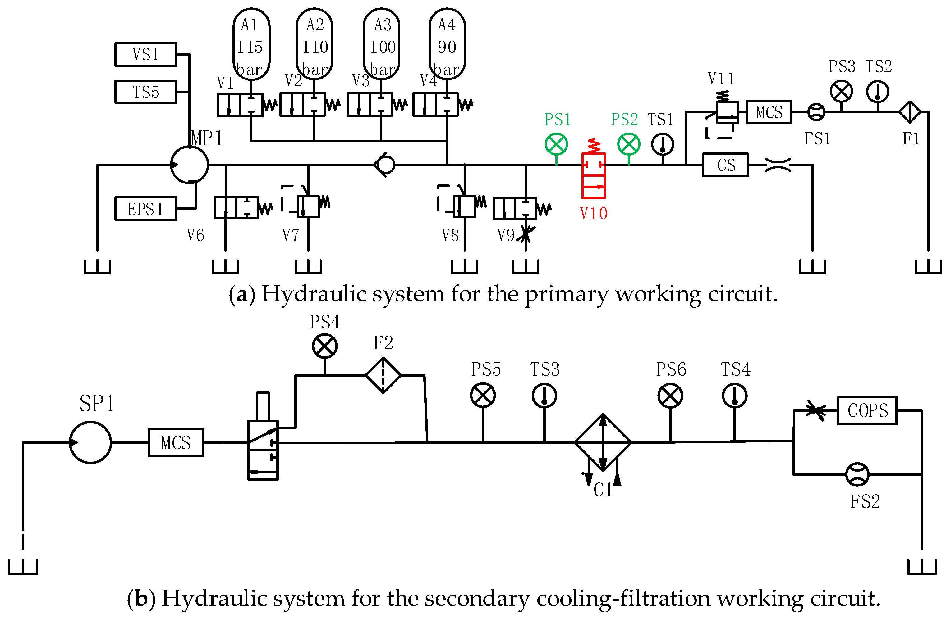
4.1. Introduction to the Experimental Platform

The experimental data sets for this study were derived from the UC Irvine Machine Learning Repository [51]. The data were collected from a hydraulic test bed that allowed a reversible change of the state or condition of various components, at the Mechatronics and Automation Technology Center of Saarbrucken University in Germany [52]. The hydraulic system consists of a primary working circuit (Figure 1a) and a secondary cooling-filtration circuit (Figure 1b), which are connected by the oil tank. In the working circuit with the main pump (electrical motor power of 3.3 kW), different load levels are cyclically repeated with the electro-hydraulic proportional valve (V11). It is possible that the typical cyclical operation and repeated load characteristic in an industrial application can be simulated by setting fixed working cycles with pre-defined load levels in the test. Meanwhile, the random load variations in mobile machines can be started by setting variable working cycles with pseudo-random load variations.

4.2. Data Acquisition System

The condition monitoring system for the hydraulic system is equipped with several sensors for measuring process values. Among them, there are six pressure sensors (PS1–PS6), two flow rate sensors (FS1, FS2), five temperature sensors (TS1–TS5), one motor power sensor (EPS1), and one vibration sensor (VS1) with standard industrial 4–20 mA current loop interfaces connected to a data acquisition system. In addition, sensors integrating EIA-232 and EIA-485 buses for oil particle contamination (CS and MCS) and oil parameter monitoring (COPS) are installed in the condition monitoring system. In total, the above 17 sensor signals are stored while the hydraulic system repeats pre-defined constant working cycles with changing conditions of hydraulic components to identify typical signal patterns. The sampling rate of the above sensors is set within the range of 1 Hz to 100 Hz, respectively, according to the different types of collected state signals. The specific sampling rate of each sensor is shown in

Table 1. Sampling rates of sensors.

Sensor	Physical Quantity	Unit	Sampling Rate	Attribute Information
PS1-6	Pressure	bar	100 Hz	Actual sensor
EPS1	Motor power	W	100 Hz	Actual sensor
FS1-2	Volume flow	L/min	10 Hz	Actual sensor
TS1-4	Temperature	°C	1 Hz	Actual sensor
VS1	Vibration	mm/s	1 Hz	Actual sensor
CE	Cooling efficiency	%	1 Hz	Virtual sensor
CP	Cooling power	kW	1 Hz	Virtual sensor
SE	Efficiency factor	%	1 Hz	Virtual sensor

.

The sensor data are connected and buffered on a Programmable Logic Controller (PLC) (Beckhoff CX5020) at run time and transferred to a computer by EtherCAT, where the data are stored for further analysis. It is possible to configure fault characterization measurements with a specifically developed tool such as LabVIEW and to, subsequently, perform them by using the PLC. Using this tool, measurements of the fault type, severity, and duration are taken, if necessary, to define different fault states, such as hydraulic pump internal leakage, hydraulic valve switching characteristic degradation, accumulator leakage, and cooler power degradation.

Table 2. Hydraulic test bed: components and their simulated fault conditions.

Hydraulic Component	Fault Conditions	Control Parameters	Possible Range
Valve (V10)	Switching characteristic degradation	Control current of V10	0 … 100% of nom. current.
Pump (MP1)	Internal leakage	Switchable bypass orifices V9	3 × 0.2 mm, 3 × 0.25 mm
Accumulators (A1–A4)	Gas leakage	Accumulators A1–A4 with different pre-charge pressures	90, 100, 110, 115 bar
Cooler (C1)	Cooling power decrease	Fan duty cycle of C1	0 … 100% (0.6 … 2.2 kW)

shows the components and respective parameters that are configurable to simulate fault scenarios. The experimental method has the advantages of not requiring damage to the mechanical structure of the hydraulic valve, repeatability, and reversibility of the fault state, and simple operation of the fault setting.

4.3. Hydraulic Valve Fault Setting and Data Acquisition

According to the primary working circuit in Figure 1a, the working cycle (duration 60 s) consists of different segments with transient and static load characteristics performed by the electro-hydraulic proportional pressure valve (V11) and the directional valve (V10) to simulate a typical machine operation. Under pre-defined load conditions, the current set points of the directional valve are 100%, 90%, 80%, and 73% of the nominal value. Thus, a simulation is conducted for the hydraulic valve (V10) in the fault states of normal, slight, medium, and severe valve operation deterioration, and raw sensor data are collected during characterization.

The specific experimental process is under different fault conditions of the hydraulic valve (V10). The hydraulic system is cyclically operated for 2205 cycles with a pre-defined load on the electro-hydraulic servo valve (V11), and the running time of each cycle is 60 s. Among them, the number of cycles in which the hydraulic system is in an unstable state is 756 cycles, and, in a steady state, it is 1449 cycles. Therefore, in the steady state, the experimental data of 369 normal states, 360 slight fault states, 360 medium fault states, and 360 severe fault states are obtained, respectively, for a total of 1449 sets of data. Taking the partial pressure signals of the inlet (PS1) and outlet (PS2) measured by the hydraulic directional valve (V10) within the fixed working cycle with a duration of 60 s as an example, the changing rule of different fault states in the steady state is shown in Figure 2.

5. Hydraulic Valve Fault Diagnosis Based on PCA and XGBoost

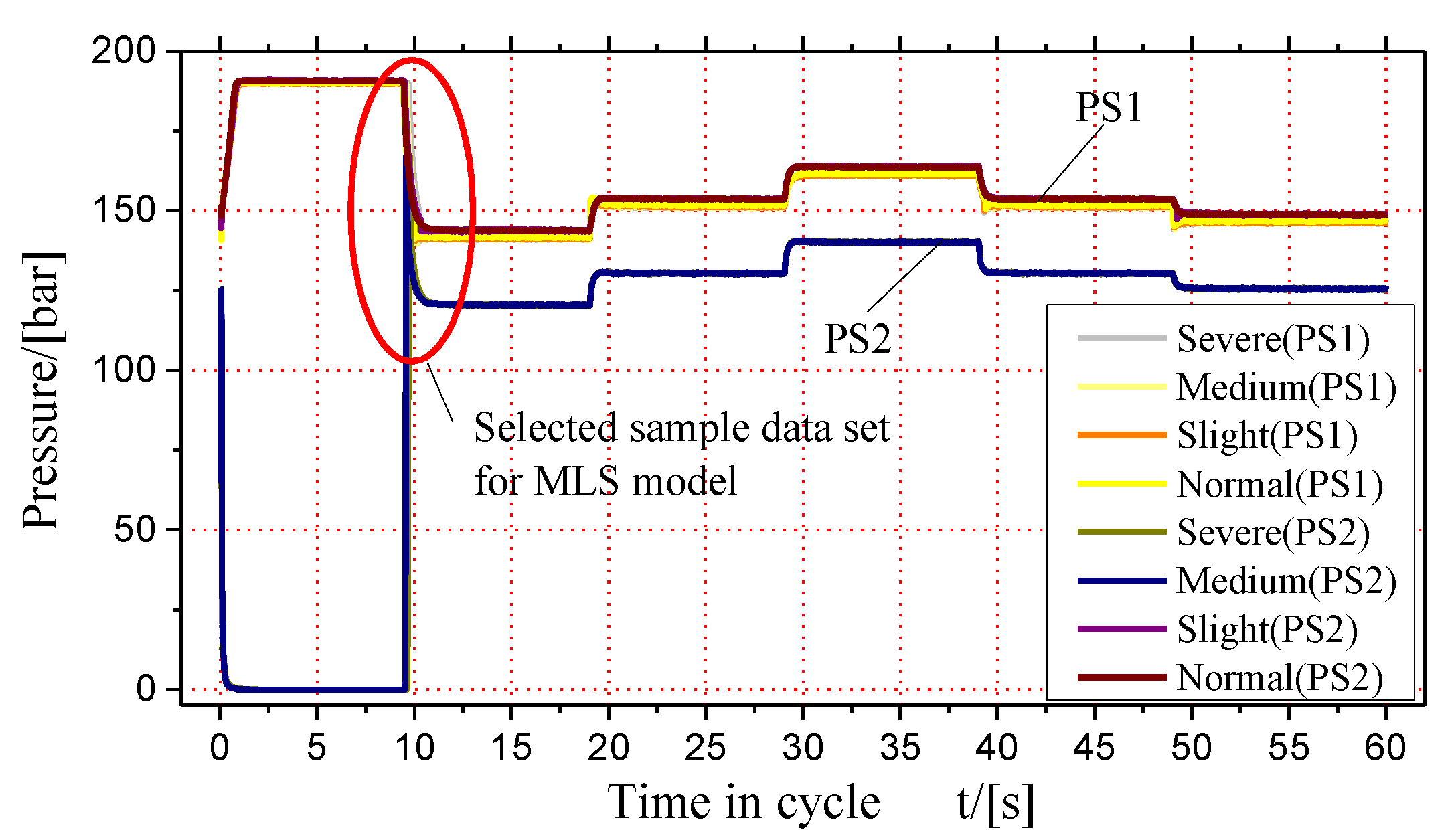
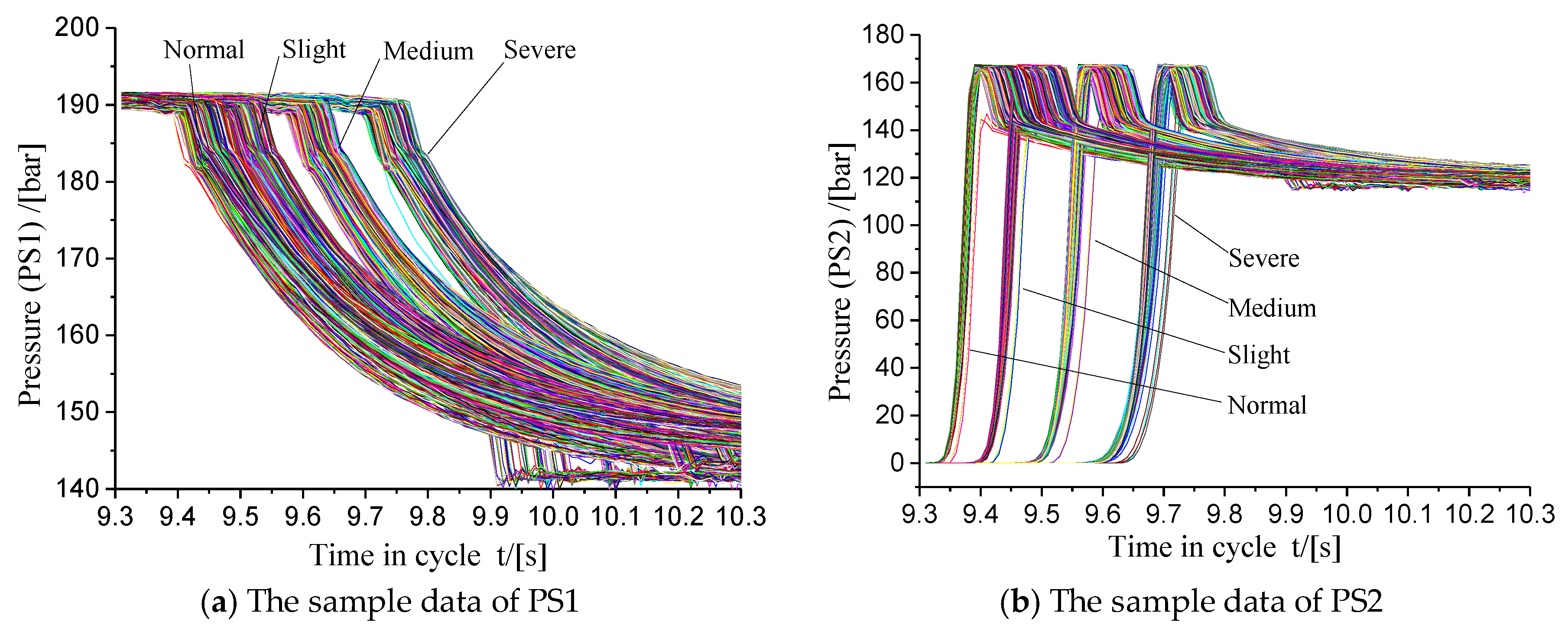
5.1. Acquisition of Sample Data for a Hydraulic Valve Fault Diagnosis

Figure 2 shows that, in each working cycle, the hydraulic directional valve (V10) is switched at about the 10th second, and the valve outlet pressure (PS2) rises rapidly when the valve inlet pressure (PS1) decreases significantly. It can be seen that the sensor data contain the fault characteristics of the hydraulic valve. As shown in Figure 3, based on the working principle and switching performance characteristics of the hydraulic valve, 100 data points between 9.3 s and 11.3 s in each cycle of PS1 (Figure 3a) and PS2 (Figure 3b) are, respectively, intercepted in the 1449 sets of data, which obtains two sample data sets of 1449 × 100 dimensions for the modeling analysis. These data sets contain the pressure changes before and after the hydraulic valve switching process.

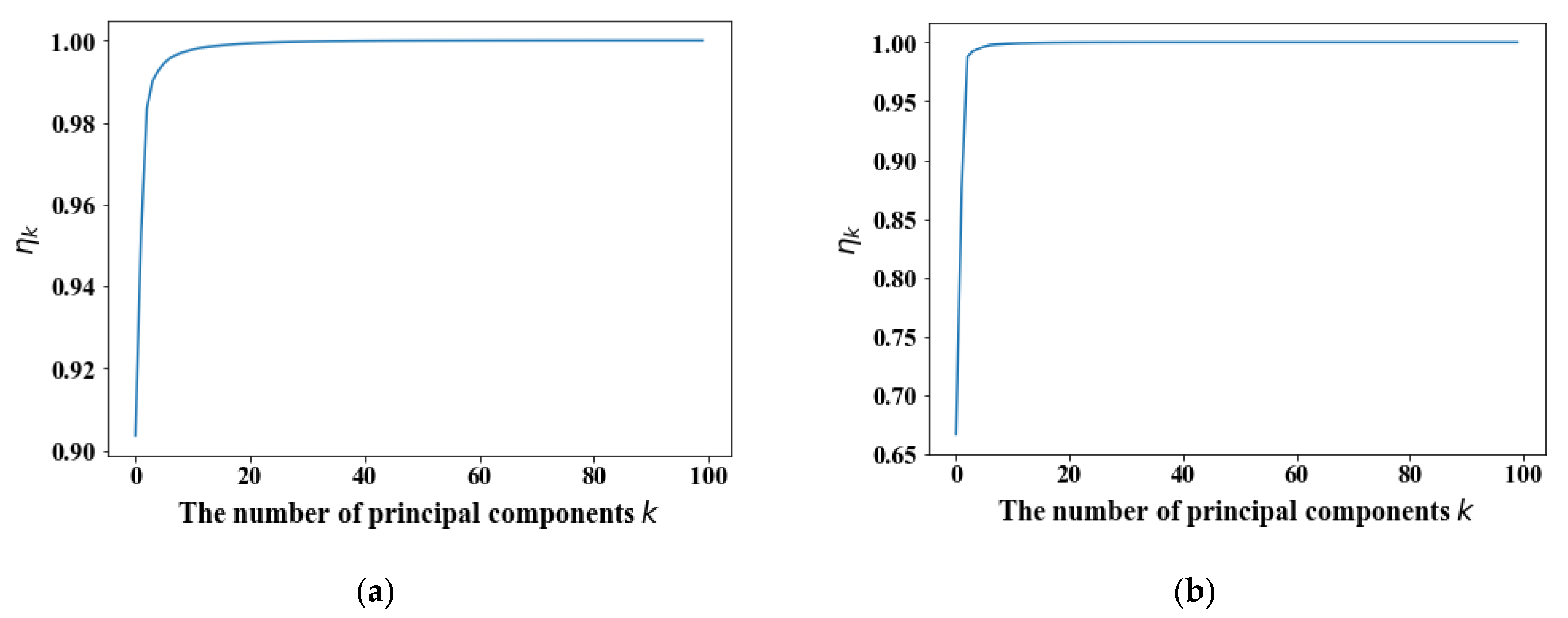
5.2. Dimensionality Reduction of a PCA-Based Training Set Sample

Dimensionality reduction of the training set sample data by the PCA method not only has the advantages of reducing the dimension of the training set and improving the speed of the model training, but also has the functions of eliminating the outliers of the signal and denoising the signal. Based on the dimensionality reduction principle and analysis steps of the PCA method described above, the variance contribution rates ${\delta }_i$ of the principal components of the PS1 and PS2 training set samples are calculated, according to Equation (16). The variance contribution rates ${\delta }_i$ of the first 1–18 principal elements are shown in

Table 3. Variance contribution of partial principal components.

Number of Principal Component	1	2	3	4	5	6	7	8	9
Unit	%	%	%	%	%	%	%	%	%
PS1	90.36	4.96	3.02	0.68	0.24	0.18	0.12	0.07	0.06
PS2	66.72	20.90	11.19	0.46	0.21	0.17	0.12	0.05	0.03
Number of Principal Component	10	11	12	13	14	15	16	17	18
Unit	%	%	%	%	%	%	%	%	%
PS1	0.04	0.04	0.03	0.02	0.01	0.01	0.00	0.00	0.00
PS2	0.03	0.02	0.02	0.01	0.00	0.00	0.00	0.00	0.00

.

According to Equation (17), the relationship between the cumulative contribution rate ${\eta }_k$ of the principal components of the PS1 and PS2 training set samples and the number of principal components is further plotted, as shown in Figure 4.

However, there is no general method to select the optimal number of principal components to be retained. In order to retain the original information to the greatest extent, the variance contribution of principal components ${\delta }_i$ is set close to 0, and the cumulative contribution rate ${\eta }_k$ is set close to 100%. According to Table 3 and Figure 4, from the variance contribution rates ${\delta }_i$ of the principal components, it can be known that, after PCA dimensionality reduction, the information of PS1 data is concentrated in the first 1–15 principal components, and the PS2 data information is concentrated in the first 1–13. Considering the balance of the model training data, the number of principal components k after dimensionality reduction to the PS1 and PS2 data sets is determined to be 15. The data set of 1449 × 100 dimensions can be compressed to 1449 × 15 dimensions. The data set after dimensionality reduction is applied to the modeling and learning process of the training sample data set, which is divided into training samples and test samples, according to a certain proportion, as displayed in

Table 4. The proportion sets of sample data for the hydraulic valve (V10).

Fault Conditions for the Hydraulic Valve	Normal	Slight	Medium	Severe	Total
The total number of samples	369	360	360	360	1449
Number of training samples	257	252	238	264	1011
Number of test samples	112	108	122	96	438

.

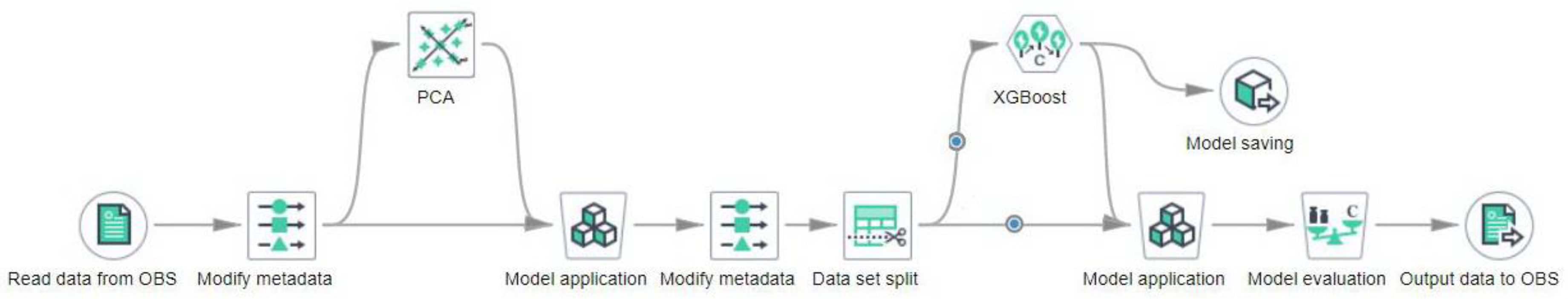
5.3. Model Establishment Based on the XGBoost Algorithm

Huawei MLS integrates multiple algorithm nodes and can combine different nodes by dragging and connecting, and creating a corresponding visual workflow for data processing, model training, evaluation, and prediction, according to research tasks. At the same time, MLS integrates the function of the Jupyter notebook, which provides users with an interactive notebook as an integrated development environment for machine learning applications. The environment supports the writing of Python scripts and performs data analysis and model building by using the Spark native algorithm MLlib. Based on the workflow, a hydraulic valve fault diagnosis model combining PCA and the XGBoost algorithm is established in MLS. The specific process is shown in Figure 5.

5.4. Model Evaluation

In the model shown in Figure 5, the training sample data are split into a training set and a test set by a “Data set split” module, and the split ratio is shown in Table 4. The test set is evaluated by the “Model Evaluation” module in the MLS. The models are quantitatively evaluated by using model evaluation indicators, such as confusion matrix, precision, recall rate, and an F1 score. The specific definitions of each indicator are as follows.

Taking the binary classification problem as an example, the sample data are divided into true positive (TP), false positive (FP), true negative (TN), and false negative (FN), according to the combination of its real category and machine learning prediction category. Then, TP + FP + TN + FN = Total number of samples.

(1) Precision

Precision indicates the proportion of the sample whose real category is positive in the sample with a positive prediction category. The calculation formula is shown below.

$$P=\frac{TP}{TP+FP}$$

(32)

(2) Recall Rate

The recall rate indicates that the proportion of the sample with a positive prediction category in the sample with a real positive category. The calculation formula is shown below.

$$R=\frac{TP}{TP+FN}$$

(33)

where the precision P and the recall rate R are a pair of contradictory indicators. In general, when the precision is high, the recall rate tends to be low. When the recall rate is high, the precision tends to be low.

(3) F1 Score

The F1 score takes the precision and recall rate into account and is their weighted harmonic mean. When the weights of precision and recall rate are the same, the harmonic mean obtained is called the F1 score, and the calculation formula is shown below.

$$F1score=2\times \frac{P\times R}{P+R}$$

(34)

(4) Confusion Matrix

The confusion matrix is used for evaluating the model when faced with a multi-classification problem, and the weight of each category is almost equal. Each column of the confusion matrix represents a prediction category, and the total number of data for each column represents the number of data predicted to be in the category. Each row represents the true attribution category of the data, and the total number of data for each row represents the number of data instances belonging to that category. For a confusion matrix, the larger the value on the diagonal is, the better the matrix. The smaller value of other locations are better.

The above-mentioned the Principal Component Analysis and eXtreme Gradient Boosting (PCA-XGBoost) model trained in the Huawei Cloud MLS is tested by the test set, and its specific indicators are shown in

Table 5. Evaluation indexes of the model using test samples.

Confusion Matrix						Precision	Recall Rate	F1 Score
	Predicted	Normal	Slight	Medium	Severe
Practical
Normal		101	11	0	0	0.990	0.902	0.944
Slight		0	108	0	0	0.885	1.000	0.939
Medium		0	3	119	0	1.000	0.975	0.988
Severe		1	0	0	95	1.000	0.990	0.995

.

It can be seen from Table 5 that the diagonal value of the confusion matrix in the hydraulic valve fault diagnosis model is much larger than the value of the non-diagonal line. The precision and recall rate of the model are all above 88%, and the F1 score is higher than 93%. The above results show that the PCA-XGBoost model has high accuracy.

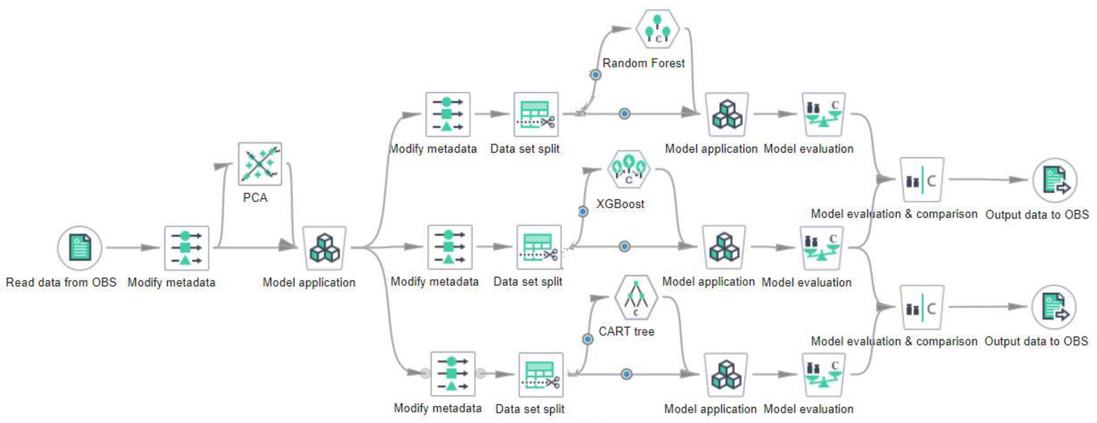
5.5. Comparison of Model Diagnosis Results

In the same environment of the Huawei Cloud MLS platform, the model constructed by the XGBoost algorithm was compared with the CART Tree classification model and the Random Forests (RFs) algorithm model. The comparison diagram is displayed in Figure 6.

The comparison is made based on the model evaluation indicators such as the precision, the recall rate, and the F1 score. Additionally, the comparison results are shown in

Table 6. Model evaluation comparison.

Model Algorithm	Fault Conditions for the Hydraulic Valve	Model Evaluation Index
		Precision	Recall Rate	F1 Score
PCA-CART	Normal	0.878	0.902	0.890
	Slight	0.914	0.889	0.901
	Medium	0.907	0.959	0.932
	Severe	0.966	0.896	0.930
	Average value	0.916	0.911	0.913
PCA-RFs	Normal	0.916	0.875	0.895
	Slight	0.909	0.926	0.917
	Medium	0.929	0.959	0.944
	Severe	0.958	0.948	0.953
	Average value	0.928	0.927	0.927
PCA-XGBoost	Normal	0.990	0.902	0.944
	Slight	0.885	1.000	0.939
	Medium	1.000	0.975	0.988
	Severe	1.000	0.990	0.995
	Average value	0.969	0.967	0.966

.

As shown in Table 6, after the principal component dimensionality reduction of the data, the CART Tree, Random Forests, and XGBoost algorithms are, respectively, used to construct the fault diagnosis model of the hydraulic valve. Afterward, the models are tested through the test set. The test results indicate that the average precision of the XGBoost model is 96.9%0.969, the average recall rate is 96.7%, and the average F1 score is96.6%. The values of the evaluation indicators are higher than those of the CART Tree and Random Forests models, which can not only prove the superiority of the algorithm, but also demonstrate the effectiveness of this algorithm for hydraulic valve fault diagnosis.

6. Conclusions

This paper mainly studies the fault diagnosis of hydraulic valves. Based on the status monitoring data of the measured inlet and outlet pressure signals of the hydraulic valve, PCA was adopted to reduce the dimensions of the data, and the XGBoost algorithm was used to construct a machine learning model for hydraulic valve fault diagnosis. By testing the evaluation indexes of the machine learning model, the effectiveness and superiority of the above method are proved. The main conclusions are as follows.

(1) In this study, the pressure signals of the hydraulic valve are utilized as the sample data for fault diagnosis in order to realize accurate diagnosis and classification of hydraulic valve faults. Then, a novel fault diagnosis method for hydraulic valves based on the variation characteristics of pressure signals is proposed.

(2) PCA dimensionality reduction for the original data set of feature vectors can not only significantly reduce the dimension of the feature vector, but also remove redundant information in the original data set. The principal component feature set after dimensionality reduction is used to train the XGBoost machine learning, in order to construct the fault diagnosis model for the hydraulic valve. The test results indicate that the precision mean of the model is 96.9%, the recall rate mean is 96.7%, and the F1 score mean is 96.6% on the test set. Compared with the decision tree and random forest models, the constructed model has higher accuracy.

(3) This research builds a fault diagnosis model for the hydraulic valve in the visual workflow of HUAWEI Cloud MLS, and carries out data processing, model training, evaluation, and prediction. In this way, hydraulic valve fault diagnosis, machine learning algorithms, and HUAWEI cloud are organically combined together, which can provide a theoretical basis and practical guidance for the remote fault diagnosis of hydraulic components and the predictive maintenance of hydraulic systems.

References

1. Schneider, T.; Helwig, N.; Schütze, A. Automatic feature extraction and selection for classification of cyclical time series data. TM-Tech. Mess. 2017, 84, 198–206. [Google Scholar] [CrossRef]
2. Goharrizi, A.Y.; Sepehri, N. Application of fast Fourier and wavelet transforms towards actuator leakage diagnosis: A comparative study. Int. J. Fluid Power 2013, 14, 39–51. [Google Scholar] [CrossRef]
3. Watton, J. Modelling, Monitoring and Diagnostic Techniques for Fluid Power Systems; Springer Science & Business Media: New York, NY, USA, 2007. [Google Scholar]
4. Qian, J.Y.; Chen, M.R.; Liu, X.L.; Jin, Z.J. A numerical investigation of the flow of nanofluids through a micro Tesla valve. J. Zhejiang Univ. Sci. A 2019, 20, 50–60. [Google Scholar] [CrossRef]
5. Qian, J.Y.; Gao, Z.X.; Liu, B.Z.; Jin, Z.J. Parametric study on fluid dynamics of pilot-control angle globe valve. ASME J. Fluids Eng. 2018, 140, 111103. [Google Scholar] [CrossRef]
6. Zhang, J.; Xia, S.; Ye, S.; Xu, B.; Song, W.; Zhu, S.; Xiang, J. Experimental investigation on the noise reduction of an axial piston pump using free-layer damping material treatment. Appl. Acoust. 2018, 139, 1–7. [Google Scholar] [CrossRef]
7. Ye, S.; Zhang, J.; Xu, B.; Zhu, S.; Xiang, J.; Tang, H. Theoretical investigation of the contributions of the excitation forces to the vibration of an axial piston pump. Mech. Syst. Signal Process. 2019, 129, 201–217. [Google Scholar] [CrossRef]
8. Wang, C.; Hu, B.; Zhu, Y.; Wang, X.; Luo, C.; Cheng, L. Numerical study on the gas-water two-phase flow in the self-priming process of self-priming centrifugal pump. Processes 2019, 7, 330. [Google Scholar] [CrossRef]
9. Wang, C.; Chen, X.; Qiu, N.; Zhu, Y.; Shi, W. Numerical and experimental study on the pressure fluctuation, vibration, and noise of multistage pump with radial diffuser. J. Braz. Soc. Mech. Sci. Eng. 2018, 40, 481. [Google Scholar] [CrossRef]
10. Zheng, H.; Wang, R.; Xu, W.; Wang, Y.; Zhu, W. Combining a HMM with a genetic algorithm for the fault diagnosis of photovoltaic inverters. J. Power Electron. 2017, 17, 1014–1026. [Google Scholar]
11. Xu, X.; Wang, W.; Zou, N.; Chen, L.; Cui, X. A comparative study of sensor fault diagnosis methods based on observer for ECAS system. Mech. Syst. Signal Process. 2017, 87, 169–183. [Google Scholar] [CrossRef]
12. Sun, H.; Yuan, S.; Luo, Y. Cyclic spectral analysis of vibration signals for centrifugal pump fault characterization. IEEE Sens. J. 2018, 18, 2925–2933. [Google Scholar] [CrossRef]
13. Tang, S.; Gu, J.; Tang, K.; Zou, R.; Sun, X.; Uddin, S. A Fault-signal-based generalizing remaining useful life prognostics method for wheel hub bearings. Appl. Sci. 2019, 9, 1080. [Google Scholar] [CrossRef]
14. Mao, Y.; Liu, G.; Zhao, W.; Ji, J. Vibration prediction in fault-tolerant flux-switching permanent-magnet machine under healthy and faulty conditions. IET Electr. Power Appl. 2017, 11, 19–28. [Google Scholar] [CrossRef]
15. Chen, T.; Chen, L.; Xu, X.; Cai, Y.; Jiang, H.; Sun, X. Passive fault-tolerant path following control of autonomous distributed drive electric vehicle considering steering system fault. Mech. Syst. Signal Process. 2019, 123, 298–315. [Google Scholar] [CrossRef]
16. Zhou, H.; Liu, G.; Zhao, W.; Yu, X.; Gao, M. dynamic performance improvement of five-phase permanent-magnet motor with short-circuit fault. IEEE Trans. Ind. Electron. 2018, 65, 145–155. [Google Scholar] [CrossRef]
17. Schneider, T.; Helwig, N.; Schütze, A. Industrial condition monitoring with smart sensors using automated feature extraction and selection. Meas. Sci. Technol. 2018, 29, 094002. [Google Scholar] [CrossRef]
18. Zhu, Y.; Tang, S.; Quan, L.; Jiang, W.; Zhou, L. Extraction method for signal effective component based on extreme-point symmetric mode decomposition and Kullback-Leibler divergence. J. Braz. Soc. Mech. Sci. Eng. 2019, 41, 100. [Google Scholar] [CrossRef]
19. Zhu, Y.; Qian, P.; Tang, S.; Jiang, W.; Li, W.; Zhao, J. Amplitude-frequency characteristics analysis for vertical vibration of hydraulic AGC system under nonlinear action. AIP Adv. 2019, 9, 035019. [Google Scholar] [CrossRef] [Green Version]
20. Wu, W.; Yang, S.; Zhou, T. Application of complex three-order cumulants to fault diagnosis of hydraulic valve. J. Tianjin Univ. 2013, 46, 590–595. [Google Scholar]
21. Gao, Y.; Huang, Y. Application of AR bi-spectrum in fault diagnosis of reducing valve. Mach. Des. Manuf. 2011, 11, 70–72. [Google Scholar]
22. Li, T.; Fan, M.; Huang, Q.; Li, Z. Research on fault diagnosis method for auto pilot hydraulic valve based on fractal theory. China Meas. Test 2012, 38, 1–5. [Google Scholar]
23. Raduenz, H.; Mendoza, Y.E.A.; Ferronatto, D.; Souza, F.J.; da Cunha Bastos, P.P.; Soares, J.M.C.; De Negri, V.J. Online fault detection system for proportional hydraulic valves. J. Braz. Soc. Mech. Sci. Eng. 2018, 40, 331. [Google Scholar] [CrossRef]
24. Vianna, W.O.L.; de Souza Ribeiro, L.G.; Yoneyama, T. Electro hydraulic servovalve health monitoring using fading extended Kalman filter. In Proceedings of the 2015 IEEE Conference on Prognostics and Health Management (PHM), Austin, TX, USA, 2015, 22–25 June 2015; IEEE: Piscataway, NJ, USA, 2015; pp. 1–6. [Google Scholar]
25. Folmer, J.; Schrüfer, C.; Fuchs, J.; Vermum, C.; Vogel-Heuser, B. Data-driven valve diagnosis to increase the overall equipment effectiveness in process industry. In Proceedings of the 2016 IEEE 14th International Conference on Industrial Informatics (INDIN), Poitiers, France, 18–21 July 2016; IEEE: Piscataway, NJ, USA, 2016; pp. 1082–1087. [Google Scholar]
26. Lei, Y.; Jia, F.; Kong, D.; Lin, J.; Xing, S. Opportunities and challenges of machinery intelligent fault diagnosis in big data era. Chin. J. Mech. Eng. 2018, 54, 94–104. [Google Scholar] [CrossRef]
27. Pei, H.; Hu, C.; Si, X.; Zhang, J.; Pang, Z.; Zhang, P. Review of machine learning based remaining useful life prediction methods for equipment. J. Mech. Eng. 2019, 55, 1–13. [Google Scholar]
28. Zhu, Y.; Jiang, W.; Kong, X.; Quan, L.; Zhang, Y. A chaos wolf optimization algorithm with self-adaptive variable step-size. AIP Adv. 2017, 7, 105024. [Google Scholar] [CrossRef]
29. Pearson, K. On lines and planes of closest fit to systems of points in space. Philos. Mag. A 1901, 6, 559–572. [Google Scholar] [CrossRef]
30. Fisher, R.A.; Mackenzie, W.A. Studies in crop variation. II. The manurial response of different potato varieties. J. Agric. Sci. 1923, 13, 311–320. [Google Scholar] [CrossRef] [Green Version]
31. Hotelling, H. Analysis of a complex of statistical variables into principal components. J. Educ. Psychol. 1933, 24, 417–441. [Google Scholar] [CrossRef]
32. Mohanty, S.; Gupta, K.K.; Raju, K.S. Adaptive fault identification of bearing using empirical mode decomposition–principal component analysis-based average kurtosis technique. IET Sci. Meas. Technol. 2017, 11, 30–40. [Google Scholar] [CrossRef]
33. Stief, A.; Ottewill, J.; Baranowski, J.; Orkisz, M. A PCA and two-stage bayesian sensor fusion approach for diagnosing electrical and mechanical faults in induction motors. IEEE Trans. Ind. Electron. 2019, 66, 9510–9520. [Google Scholar] [CrossRef]
34. Caggiano, A. Tool wear prediction in Ti-6Al-4V machining through multiple sensor monitoring and PCA features pattern recognition. Sensors 2018, 18, 823. [Google Scholar] [CrossRef] [PubMed]
35. Wang, Y.; Ma, X.; Qian, P. Wind turbine fault detection and identification through PCA-based optimal variable selection. IEEE Trans. Sustain. Energy 2018, 9, 1627–1635. [Google Scholar] [CrossRef]
36. Xiao, X.; Zhao, S.; Chen, K.; Zhang, M.; Liu, L. Application of principal component analysis in fault diagnosis of electro-hydrostatic actuators. Missiles Space Veh. 2019, 366, 98–104. [Google Scholar]
37. Riba, J.R.; Canals, T.; Cantero, R. Recovered paperboard samples identification by means of mid-infrared sensors. IEEE Sensors J. 2013, 13, 2763–2770. [Google Scholar] [CrossRef]
38. Chen, T.; Guestrin, C. Xgboost: A scalable tree boosting system. In Proceedings of the 22nd Acm Sigkdd International Conference on Knowledge Discovery and Data Mining ACM, San Francisco, CA, USA, 13–17 August 2016; pp. 785–794. [Google Scholar]
39. Nielsen, D. Tree Boosting with XGBoost-Why Does XGBoost Win “Every” Machine Learning Competition? Master’s Thesis, Norwegian University of Science and Technology, Trondheim, Noreg, 2016. [Google Scholar]
40. Zhang, D.; Qian, L.; Mao, B.; Huang, C.; Huang, B.; Si, Y. A data-driven design for fault detection of wind turbines using random forests and XGBoost. IEEE Access 2018, 6, 21020–21031. [Google Scholar] [CrossRef]
41. Chakraborty, D.; Elzarka, H. Early detection of faults in HVAC systems using an XGBoost model with a dynamic threshold. Energy Build. 2019, 185, 326–344. [Google Scholar] [CrossRef]
42. Zhang, R.; Li, B.; Jiao, B. Application of XGBoost Algorithm in Bearing Fault Diagnosis. IOP Conference Series: Materials Science and Engineering; IOP Publishing: Bristol, UK, 2019; Volume 490, p. 072062. [Google Scholar]
43. Nguyen, H.; Bui, X.N.; Bui, H.B.; Cuong, D.T. Developing an XGboost model to predict blast-induced peak particle velocity in an open-pit mine: A case study. Acta Geophys. 2019, 67, 477–490. [Google Scholar] [CrossRef]
44. Pan, B. Application of XGBoost algorithm in hourly PM2. 5 concentration prediction. IOP Conference Series: Earth and Environmental Science; IOP Publishing: Bristol, UK, 2018; Volume 113, p. 012127. [Google Scholar]
45. Liu, Y.; Qiao, M. Heart disease prediction based on clustering and XGboost. Comput. Syst. Appl. 2019, 28, 228–232. [Google Scholar]
46. Fitriah, N.; Wijaya, S.K.; Fanany, M.I.; Badri, C.; Rezal, M. EEG channels reduction using PCA to increase XGBoost’s accuracy for stroke detection. In Proceedings of the AIP Conference, 10–11 July 2017; AIP Publishing: Melville, NY, USA, 2017; Volume 1862, p. 030128. [Google Scholar]
47. Zhao, W.; Dong, L. Machine Learning; Posts & Telecom Press: Beijing, China, 2018. [Google Scholar]
48. Zhang, J. Multivariable Statistical Process Control; Chemical Industry Press: Beijing, China, 2000. [Google Scholar]
49. Wang, G. Principal Component Analysis and Partial Least Square Method; Tsinghua University Press: Beijing, China, 2012. [Google Scholar]
50. Wang, X. A Research on CTR Prediction Based on Ensemble of RF, XGBoost and FFM; Zhejiang University: Hangzhou, China, 2018. [Google Scholar]
51. Available online: http://archive.ics.uci.edu/ml/datasets/Condition monit-oring of hydraulic systems (accessed on 26 April 2018).
52. Helwig, N.; Pignanelli, E.; Schütze, A. Condition monitoring of a complex hydraulic system using multivariate statistics. In Proceedings of the 2015 IEEE International Instrumentation and Measurement Technology Conference (I2MTC), Pisa, Italy, 11–14 May 2015; IEEE: Piscataway, NJ, USA, 2015; pp. 210–215. [Google Scholar]
Figure 1. Schematic diagram of condition monitoring in hydraulic systems.
Processes 07 00589 g001
Figure 2. Fixed working cycle (measured by partial PS1 and PS2) with a pre-defined load.
Processes 07 00589 g002
Figure 3. The sample data of the hydraulic valve fault diagnosis.
Processes 07 00589 g003
Figure 4. The cumulative contribution rate for the sample data. (a) The cumulative contribution rate η k of PS1 training set samples; (b) The cumulative contribution rate η k of PS2 training set samples.
Processes 07 00589 g004
Figure 5. The model of principal component analysis (PCA) and eXtreme Gradient Boosting (XGBoost).
Processes 07 00589 g005
Figure 6. Model comparison analysis.
Processes 07 00589 g006