1. Introduction
Over the past two decades, aseptic processing has been successfully implemented in the food processing industry, as it produces better quality food products (in terms of, e.g., texture, flavor, or color) compared to traditional canned products. In this process, the food product undergoes a continuous sterilization process, after which it is packed into a package in a sterile environment. Because of this method’s effectiveness and successful implementation with liquid food products, notably fruit juices, the application of this process to solid-liquid food mixtures (e.g., fruit pieces in juices or vegetable soup with potatoes) has been of great interest to the food processing industry. To ensure that the particles receive sufficient amounts of heat, the lethality value has to be known during the process. However, it is quite tedious and time consuming for the food processor to determine the lethality level experimentally during the aseptic process. Mathematical modeling offers an alternative method of estimating the lethality level and investigating the sterilization process of a particle in the particulate liquid food products. This approach has been used by several researchers to determine the temperature profile and lethality value in the particulate liquid foods. For example, Sastry and Cornelius [
1] solved the partial differential equation (PDE) describing the heat transfer mechanism for spherical particles and the Newtonian fluid mixture inside a scraped heat exchanger system using an algorithm written in the C++ program. According to existing literature, two important factors need to be considered in the model: the particle residence time and the heat transfer coefficient between the fluid and the particle surface. However, only one mathematical model has been described for any type of heat exchanger used in the process. Little attention has also been paid to the particle concentration effect and the radial position of the particle in the pipe during the sterilization process. In the present study, a mathematical model is implemented specifically for the sterilization of cubic food particles in liquid food flowing through a tubular heat exchanger system. Based on our comparison with an experimental case and simulation data, additional process parameters, such as particle radial positions in the pipe and concentrations, played an important role in determining the sterilization value of the product.
In the continuous sterilization process of fluid foods containing particles, heat is transferred to the suspended particles in several steps. First, external heat from a heating medium is applied to the fluid to increase its temperature rapidly in the heating section. Then, the particles are heated by heat transfer from the outer fluid. Heat penetration into the particles occurs by conduction, which is generally a much slower process for large food particles. In the next step, particle heating continues in the holding tube, where adiabatic heat exchange takes place between the fluid and solid particle [
2]. Finally, the particulate liquid product is cooled in the cooling section to avoid over-sterilization and subsequent loss in food quality. Generally, in the food industry, the temperature history of the products has to be known to evaluate the sterilization value or lethality for the assurance of the microbiological safety of the products. The main problem typically lies in the solid particles especially at the geometrical center position in the product, where a sufficient heat treatment or minimum sterilization value must be assured. It is difficult to measure the temperature in the center of the suspended particles in a liquid carrier, as the particles are hydraulically conveyed through the process equipment. Therefore, mathematical models can be applied as an appropriate tool to describe the sterilization process, which is useful for process design and, more importantly, prediction of the particle dynamics and spatial and temporal variations in temperatures of the particles moving throughout the continuous process system.
Several works have been published between the 1970s and the 2007s for modeling the continuous sterilization of solid-fluid food products. De Ruyter and Brunet [
3] developed a model for a food product containing spherical particles processed in a scraped surface heat exchanger system. In their model, an analytical solution to the PDE of heat conduction in the particle was implemented. The researchers assumed an infinite fluid-to-particle heat transfer coefficient, where the particle surface temperature was approximately the same as that of the fluid (small convective heat transfer resistance) and a linearly fluid temperature profile of the heat exchanger between the inlet and outlet. However, this model also did not specify the particle time distribution or the velocity in the system, which is particularly important for laminar flow in the tube system. Manson and Cullen [
4] developed a model for cylindrical particles in a processing system for a scraped surface heat exchanger. They implemented the finite difference method with a linearly-increasing product temperature profile between the inlet and outlet as the boundary condition in the heating section and assumed an infinite fluid-to-particle heat transfer coefficient. Additionally, the influence of product residence time was considered in the model. Sastry [
5] used the finite difference method to model the continuous sterilization process of low-acid foods containing particles for the scraped surface heat exchanger system. It was assumed that the particle moves at the same velocity as the fluid carrier; thus, the worst-case value of the fluid-to-particle heat transfer coefficient was used, which corresponds to a Nusselt number of two. Chang and Toledo [
2] also employed a finite difference method to evaluate the temperature of sweet potato particles suspended in water in the scraped surface heat exchanger system. The fluid temperature in the heating section was assumed to increase exponentially along the direction of the flow. The researchers assumed certain values of the fluid-to-particle heat transfer coefficient (239 W/m
K and 303 W/m
K), which they determined experimentally using fluid flow for the stationary single particle method. Sastry and Cornelius [
1] implemented a numerical approach to solve the energy balance of a fluid medium in the heating, holding, and cooling section and the one-dimensional heat conduction equation in spherical particles. They also assumed that the fluid mixed perfectly in the radial direction. Thus far, the above-mentioned model approaches were implemented for the scraped surface heat exchanger system, where rotating blades were used to mix the particulate liquid products. Therefore, the fluid medium was perfectly mixed in the radial direction of the heat exchanger and had a plug flow velocity profile. Sandeep, Zuritz, and Puri [
6] introduced a mathematical model for the tubular heat exchanger system, where they assumed that the fluid temperature was efficiently mixed in the radial direction of the pipe. They used the finite element method to determine spherical particle temperature profiles, as the particles move through the sterilization processing equipment. Their approach was similar to that of Sastry and Cornelius [
1]. A current mathematical model written in a Fortran program from Stoforos and Sawada [
7] was implemented for liquid food containing spherical particles in a scraped heat exchanger system. Analytical solutions were provided for determining fluid and particle temperatures. It was moreover assumed that the flowing fluid was efficiently mixed in the radial heat exchanger direction and that the particles traveled with the same average velocity of the fluid.
Some important issues, which have not been addressed so far in the above-mentioned studies, are as follows. A calculation model for the tubular heat exchanger system in the heating section is still missing, addressing the scenario where the fluid temperature varies assumedly in the radial direction of the pipe, where laminar flow typically prevails. This should be considered, as there is no mixing mechanism such as a rotating blade within the pipe. The particles will be exposed to different temperatures, depending on their radial and axial positions within the pipe. Another issue is regarding the fluid-to-particle heat transfer coefficient. All studies, with the exception of [
1], employed constant heat transfer coefficient values, which were either taken from their experimental work or from assumptions of the worst-case scenario. This coefficient is typically obtained from the Nusselt number correlation, where it is based on the relative velocity between the particle and the fluid. This calculation approach was used in [
1] for spherical particles. Apart from that, there were no particle concentration or fluid voidage effects considered in the heat transfer coefficient calculation. Lastly, the presented models were not verified or compared with any experimental data from a complete or pilot plant conducting the continuous sterilization process. Only the study in [
5] performed verification of the accuracy of the conduction heat transfer solution for particles by comparing the calculated particle temperature profile with an experimental profile from a canned product heating process. To date, no studies have been performed on the verification of the mathematical model, especially for non-spherical particles with the experiments from a continuous sterilization facility. Hence, we would like to consider these issues in the current model.
The main purpose of this study is to develop a mathematical model for the sterilization process of particulate liquid foods containing coarse particles (in the millimeter range) and evaluate the effect of heat treatment on the particles and fluid. The model simulates a continuous sterilization processing system comprised of tubular heat exchangers connected with U-bends for the heating section, constant diameter holding tubes, and a cooling section. The particulate is modeled as a cubically-shaped fruit piece, and the carrier fluid is regarded as a Newtonian fluid. The model includes the following considerations and concepts that have been highlighted in the previous paragraph:
A simplified mathematical model that solves the energy equation for the liquid and particle, which can be calculated or defined in mathematical software (e.g., MATLAB or Octave).
An analytical approach is used for the fluid temperature calculation in each straight pipe, especially in the heat exchanger. The bending effect is considered on the fluid temperature inlet at each straight section, whereas its effect on the particle temperature profile is not taken into account.
The fluid-to-particle heat transfer coefficient is determined based on the relative velocity in the system and particle concentration in the process. Here, the relative velocity is determined as the difference between the fluid and particle velocities.
A numerical approach is suitable for solving the heat transfer conduction within the particle, as the boundary condition (fluid temperature) changes within the system [
2].
From the proposed model, the objectives of this study are to (i) determine the temperature profile and fluid profiles in the continuous sterilization system from the tubular heat exchanger system, (ii) evaluate the process and product parameter effect on the temperature and lethality values or sterilization values, and (iii) compare lethality values with an experimental case study from a continuous sterilization facility.
2. The Mathematical Model
Ideally, the model would be able to predict the location, velocity, and temperature of particles spatially and temporally distributed throughout the sterilization system. This case poses a significant computational challenge, as momentum and heat transfer equations need to be solved simultaneously for the entire fluid domain and for every solid particle. Computational fluid dynamics-discrete element method (CFD-DEM) simulations are capable of handling this kind of multiphase system; however, this is time consuming for large- or industry-scale systems or if parametric studies need to be performed [
8]. Because our primary objective is the achievement of process safety, which is related to the time temperature history of the particles, particularly the temperature of the fastest moving particulates at its geometric center, the model can be simplified by solving the energy transport equations for both liquid and solid phases. The particle dynamics information, such as particle position and residence time, is necessary to solve this simplified model.
The aim is to predict the temperature history of discrete solid particles during thermal processing of liquid-particle food systems. Basic simplifying assumptions for the mathematical description of this problem include the following:
The heat transfer equation for the fluid phase is solved first, upon which the heat transfer equation of the particles is solved using the information of the calculated fluid temperature within the pipe as a boundary condition.
Heat transfer within particles occurs purely by conduction.
A three-dimensional heat transfer problem for the fluid temperature in the pipe (radial and axial directions) and a cubically-shaped particle are considered for food particles.
The thermo-physical properties for both fluid and particles are constant.
For continuous sterilization systems, we assume that the processing fluid is under steady-state conditions and experiences laminar flow; the particle travels with a certain velocity, which is determined from its residence time in the system, and the fluid temperature varies within each cross-section of the processing system (e.g., radially and axially within the tubular heat exchangers and the holding tube).
The particle radial position in the pipe of the aseptic processing system remains the same as it travels along the straight pipe and the U-bend pipe system.
The initial product temperature (before the product enters the heating section) is constant. This suggests that initial particle and fluid temperatures are constant and equal.
2.1. Heat Transfer within the Particle
The conduction heat transfer equation for heated moving particles is provided by [
1]:
where
T,
t,
,
, and
are the temperature, time, density, heat capacity, and thermal conductivity of the particle, respectively. To solve this equation, we need to provide the surface condition or boundary condition, which is given as follows:
where the fluid temperature
depends on the particle location and residence time within the pipe system. Moreover, the fluid-to-particle heat transfer coefficient
is also required, and
is the outward unit normal vector to the surface of the particle. The calculations of
and
are discussed further in the following section. The solution of Equation (
1), subject to the condition of Equation (
2), yields the temperature distribution and history of the particle. One specific temperature location is of interest, namely the geometric center of the particle, which corresponds to the slowest heating point for the lethality calculation.
2.2. Wall-to-Fluid Heat Transfer in the Heating, Holding, and Cooling Section
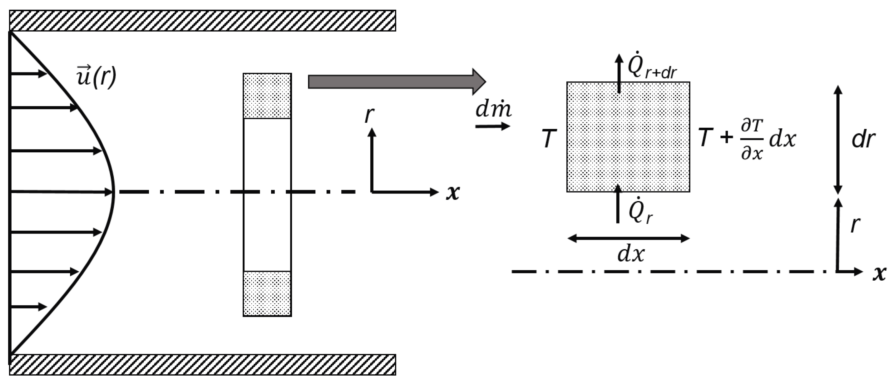
The fluid temperature medium is important for the determination of the particle temperature, as it is a function of the location within the heating, holding, and cooling section. Here, we adopt the analytical solution of laminar fluid flow in a circular pipe, which can be implemented for the tubular heat exchanger with a monotube configuration. Typically, a heat exchanger system from a continuous sterilization process is composed of a certain number of straight pipes, which are connected by U-bend pipes.
2.2.1. Heating Section
In this section, we assume that the fluid temperature is varied radially across the cross-section of the heater and along the flow direction. In an enclosed tube flow system, the energy balance can be applied for the fluid, and the following assumptions are made: steady-state flow, no thermal energy generation, negligible viscous dissipation, negligible heat conduction in the axial direction of fluid flow, fully-developed flow in the pipe, incompressible fluid, and constant heat flux on the pipe wall along the straight section. A counterflow heat exchanger with a constant product flow rate is typically used in this case; therefore, it is reasonable to assume a constant heat flux at the wall of the pipe [
9]. These assumptions lead to the simplified thermal energy equation for steady states, which can be written as (for more detail, refer to [
10]):
where
is the heat transfer rate and the right side represents the net of thermal energy for the incompressible fluid, which is calculated from the mass flow rate
, specific heat capacity
, and temperature difference between
and
.
We neglect the effect of axial conduction, and the heat transfer,
, is only due to conduction in the radial direction
r, such that Equation (
3) can be applied to the annular fluid element of
Figure 1. Additionally, the advection heat transfer occurs only in the axial direction
x. Thus, Equation (
3) leads to Equation (
4), which expresses a balance between radial conduction and axial advection heat transfer:
The differential mass flow rate in the axial direction is
, and the radial heat transfer rate is
. Assuming constant properties, Equation (
4) becomes the following steady-state differential equation describing the fluid temperature for laminar flow in a pipe with constant wall heat flux [
10]:
The suitable boundary conditions are as follows [
9]:
When a fully-developed velocity profile (
) is assumed in the axial direction as illustrated in
Figure 1, the following relation is the result:
After substituting Equation (
7) in Equation (
5), the separation of variables and the integration operation of Equation (
5) with respect to
r, and using boundary conditions from Equation (
6), the desired temperature profile takes the form [
9,
10]:
where
r,
,
x,
,
,
, and
are the radial position in the pipe, the radius of the pipe, the axial position along the pipe, the mean fluid temperature along the axial direction, the fluid temperature at the pipe wall, the mean fluid velocity in a pipe, and the fluid thermal diffusivity, respectively.
varies linearly with the axial position along the tube (
x), and
is constant. The
r value varies from the center of the pipe
to the wall of the pipe
. From Newton’s law of cooling, the fluid temperature at the wall
is given as follows:
Here,
and
are the heat flux and heat transfer coefficient near a pipe wall, respectively. The mean fluid temperature in the pipe along the axial direction is calculated as follows:
where
P is the surface perimeter for a circular pipe,
is the product mass flow rate,
is the initial temperature, and
is the fluid specific heat capacity.
is a convenient reference temperature for internal flows and mixed mean fluid temperature (the same principle used for the fluid mean velocity in a pipe), which is useful for characterizing the average thermal energy states of fluid flow in a pipe.
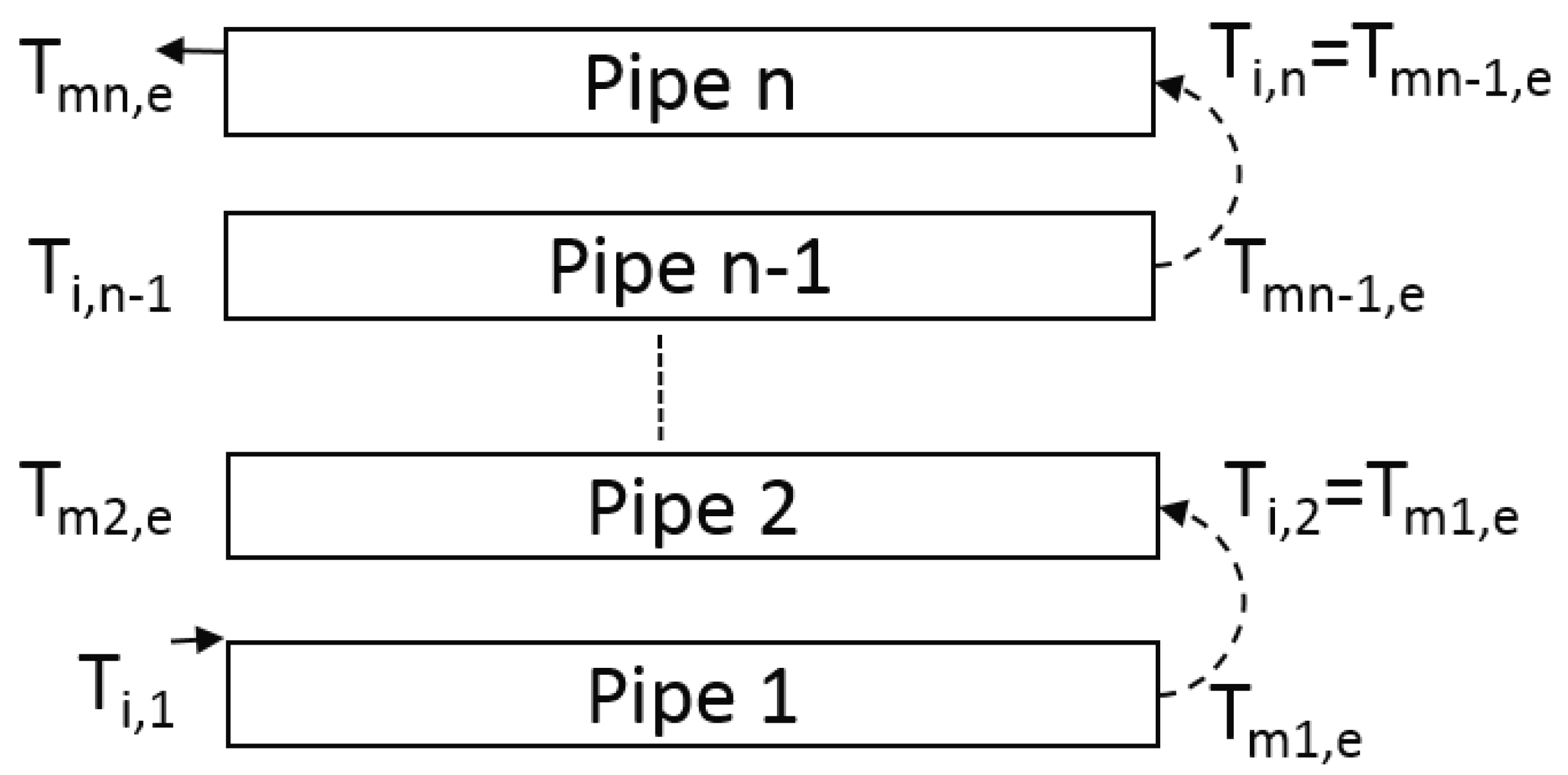
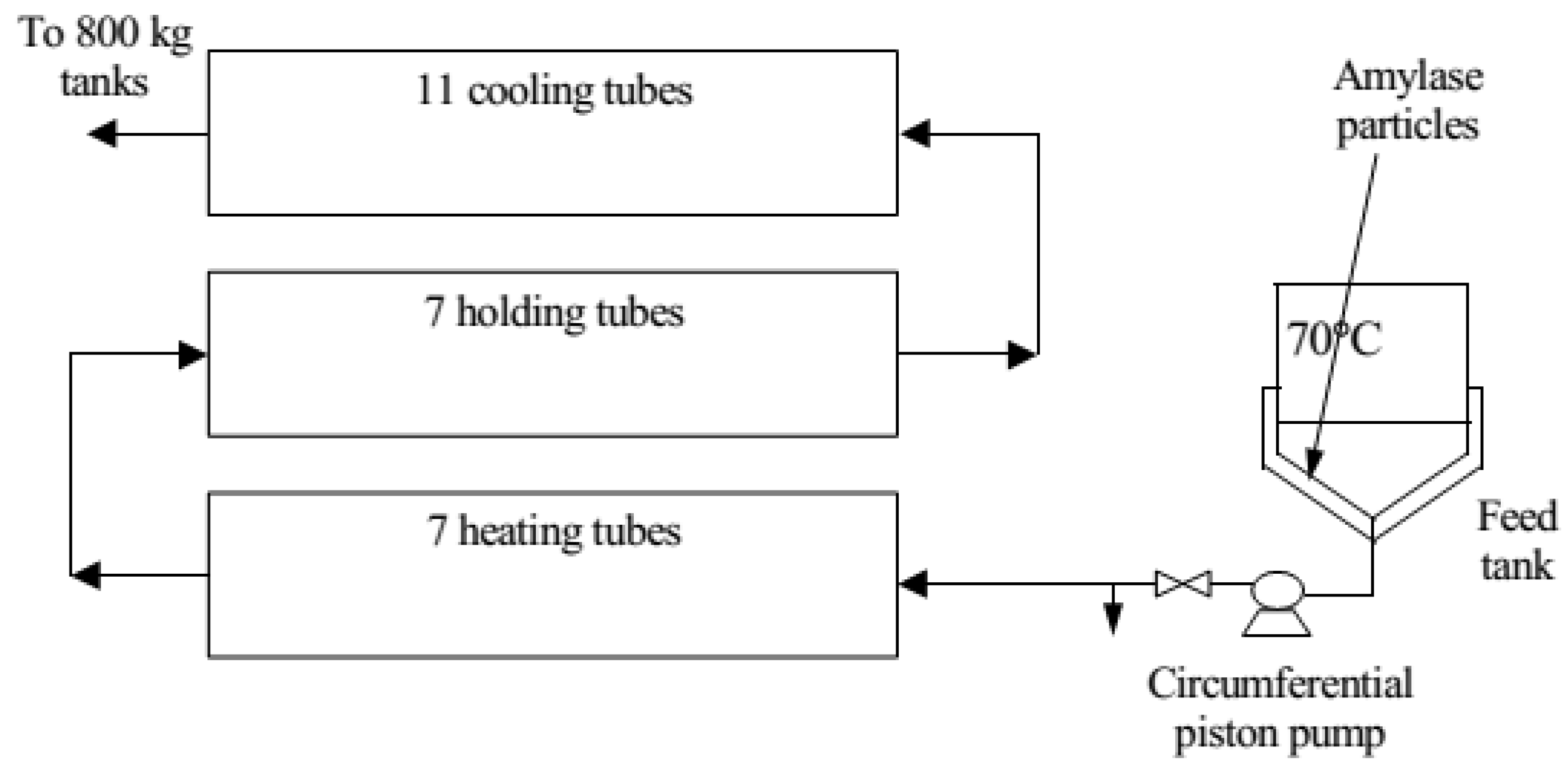
When straight pipes in the heat exchanger systems are connected with U-bends, the secondary flow occurs in bends, which potentially cause a flow mixing effect. Furthermore, it can be assumed that the thermal entry length region dominates at the entrance within each straight pipe [
11,
12]. Therefore,
at the exit of each straight pipe will be considered as the inlet temperature for the next straight pipe in the heating section, as illustrated in
Figure 2. For example, the exit temperature at Pipe 1 is the mean fluid temperature at the outlet of Pipe 1
, which consequently becomes the inlet temperature for Pipe 2. For the case of the thermal entry region,
values vary along the pipe length, and they can be determined from the Nusselt number using the following equation [
13]:
where
is the dimensionless axial position in the pipe, derived from the axial position in the pipe (
x), pipe diameter (
D), and the fluid Reynolds number (
) in the pipe:
The Reynolds number inside the pipe can be determined as follows [
13]:
2.2.2. Holding Tube
The mean fluid temperature flowing out from the heater is considered to be the inlet temperature entering the holding pipe, which is constant across the radial and axial directions of this section. We assumed that no heat loss to the surrounding occurs, since the holding tube pipes are insulated.
2.2.3. Cooling Section
During the cooling process in the counterflow tubular heat exchanger, the liquid loses heat to the cooling water. Similarly, in the heating section, a constant heating flux is used, and it is assumed that the radial temperature variation within the fluid is negligible. Equation (
10) is used to determine
in the cooling stage.
2.3. Heat Transfer Coefficient
The fluid-to-particle and the wall-fluid heat transfer coefficients are crucial design parameters for aseptic processing. Here, we first discuss the calculation methods of the fluid-to-particle heat transfer coefficient. The calculation of the wall-fluid heat transfer coefficient was already discussed in
Section 2.2. The boundary condition in Equation (
2) requires the value of the heat transfer coefficient from the liquid to the particle surface
. This coefficient is determined from the Nusselt number of the particles. A considerable number of studies are available that provide correlations for the Nusselt number as a function of other dimensionless numbers, such as the Reynolds and Prandtl numbers. A review from [
14] contains several correlations for certain cases of particulate flows. For our case, we use the following correlation for a single particle:
The particle’s Reynolds number is given as follows [
2]:
where
,
,
, and
are the fluid density, relative particle velocity, particle size, and fluid viscosity, respectively.
is the relative velocity between the particle velocity
and the fluid velocity
, which is the slip velocity that controls the interfacial heat transfer between fluid and particle.
is calculated depending on the given particle normalized residence time
, which is defined as follows [
15]:
is defined as the ratio of the particle residence time
to the mean product residence time
[
15].
When the particle travels at a velocity that is the same as the mean product velocity in the pipe, its
value is equal to one, whereas for the fastest traveling particle (2
),
can reach a value of 0.5. If a situation involves a slow-moving particle,
is greater than one. These values can be determined experimentally, as there is no correlation available for predicting the residence time as a function of process variables. The
s in the tubular pipe from several experimental studies were presented in [
1,
15], where their values varied widely among different studies, depending on the experimental setup and product characteristics. It is also worthwhile to mention that the particle radial position depends on the
s. Based on our assumption of the parabolic fluid velocity profile, the fastest particle passes through the center of the pipe
, whereas the non-center position
in the pipe is valid for
. The Prandtl number is given by the following equation:
The fluid-to-particle heat transfer coefficient
can be determined from the Nusselt number, which is defined as:
When the effect of the presence of other particles on the heat transfer is considered, the volume fraction of the fluid (void fraction) in the products is considered through the following relationship [
16]:
2.4. Lethality Calculation
Once the temperature distribution within the particle is obtained, the lethality value
of aseptic processing can be determined using Equation (
21) [
17]. In the food industry, this value is used to quantify bacteria death rates in the pasteurization or sterilization processes. This can be defined as the time, at a constant temperature,
, that produces the same destructive effect as the actual thermal process. Here,
z denotes the number of degrees of temperature change necessary to change the
value by a factor of 10, which is defined as the time required at a certain temperature to reduce the microbial population by 90% or by a factor of 10. The lethality is typically determined based on the temperature profile of the slowest heating spot, which is the particle center temperature. Comparison of the calculated
values of an entire process, with the time required to destroy a given percentage of the target microbial population (the target
value), is the basis for the thermal process design. For instance, the
target value for the
Clostridium botulinum spore in a sterilization process at a temperature of 121.1
C should be at least 6 min [
17]:
2.5. Modeling Step
Generally, providing the solution to a system comprising differential equations of the two phases, i.e., a coupled problem, represents a difficult task, since particle and fluid temperatures cannot be obtained independently. Several solution methods for a given particle shape have been presented in the literature ([
1,
2,
3,
4,
5,
6,
7]) for continuous sterilization of particulate liquid food products. In our case, we implemented a simplified solution, where the equations of each phase are solved separately. In general, the following main steps were implemented:
Analytical solutions were used for steady-state fluid temperature profiles in the absence of particles in the heating, holding, and cooling sections.
Numerical methods (e.g., finite difference method [
18] or MATLAB PDE solver [
19]) were employed to solve the transient heat conduction equation for the particle. The fluid temperature was taken from Step 1 a according to the particle position and residence time, which is required for the boundary condition. In our simulation, we used the MATLAB PDE tool, which provides functions for solving structural mechanics, heat transfer, and general PDEs using finite element analysis.
Once the temperature profile of the particle, particularly the particle center temperature, has been calculated, the lethality value at this position can be determined.
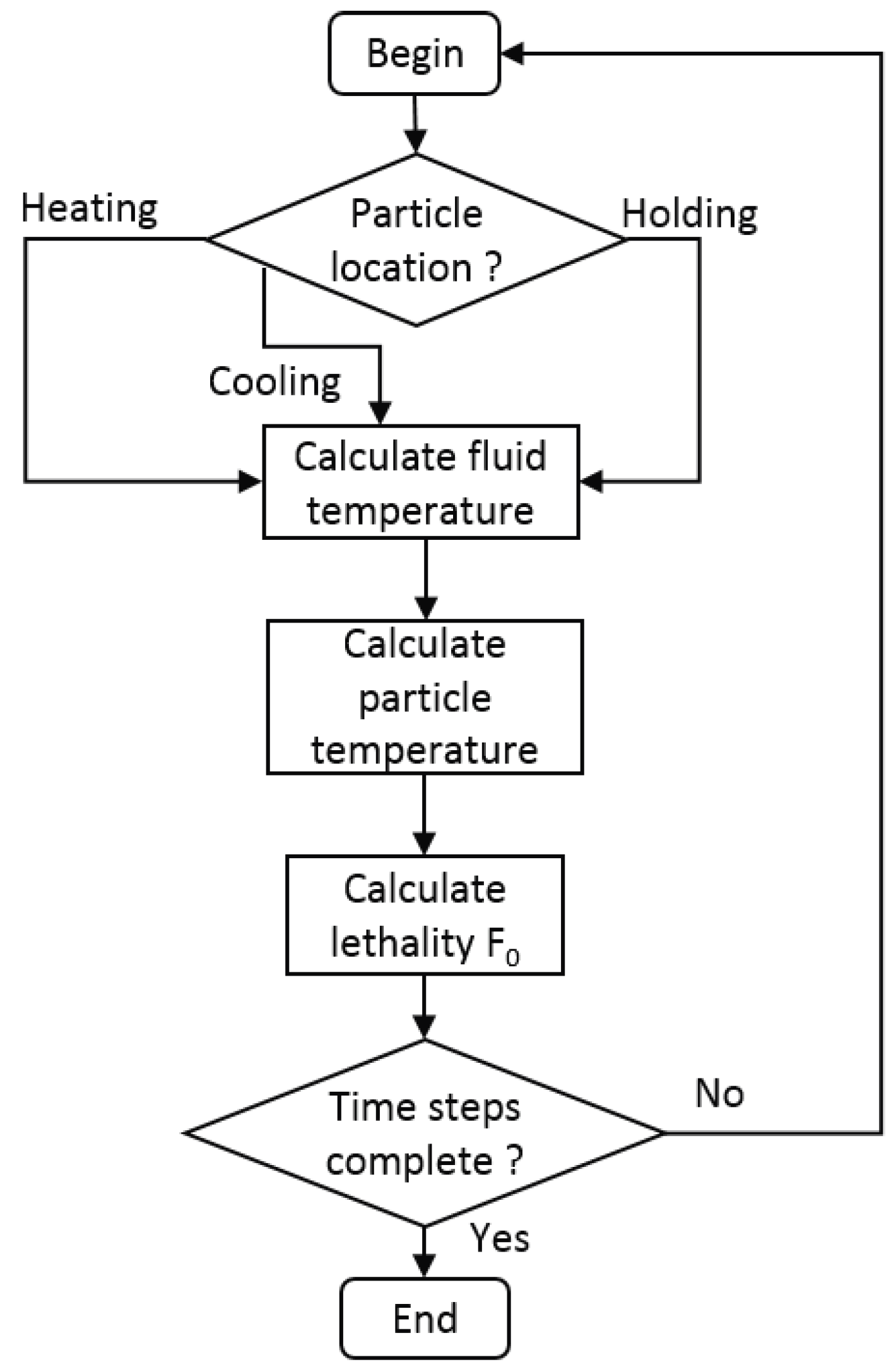
The flowchart in
Figure 3 summarizes the calculation steps of the particle temperature for the aseptic processing. In these simulations, the fluid temperature determined in Step 1 a was used to represent the external environment experienced by the investigated particle. The particles’ and the fluid’s physical properties, characteristics, and process parameters can be made to correspond to those encountered in real product processing conditions. A certain scenario could be simulated in terms of the particle residence time and the particle flow position in the pipe. This is discussed further in
Section 3.
2.6. Model Performance Analysis
For the evaluation of model, we determined the difference between the simulated value and the experimental value as a percentage of the experimental value. Percent deviation was used to measure the difference between the model prediction and the experimental value. It is presented in percentages:
Here, and are the predicted value of the y variable and the experimental value of the y variable, respectively. In our simulation cases, the y variables are the temperature and the lethality value.
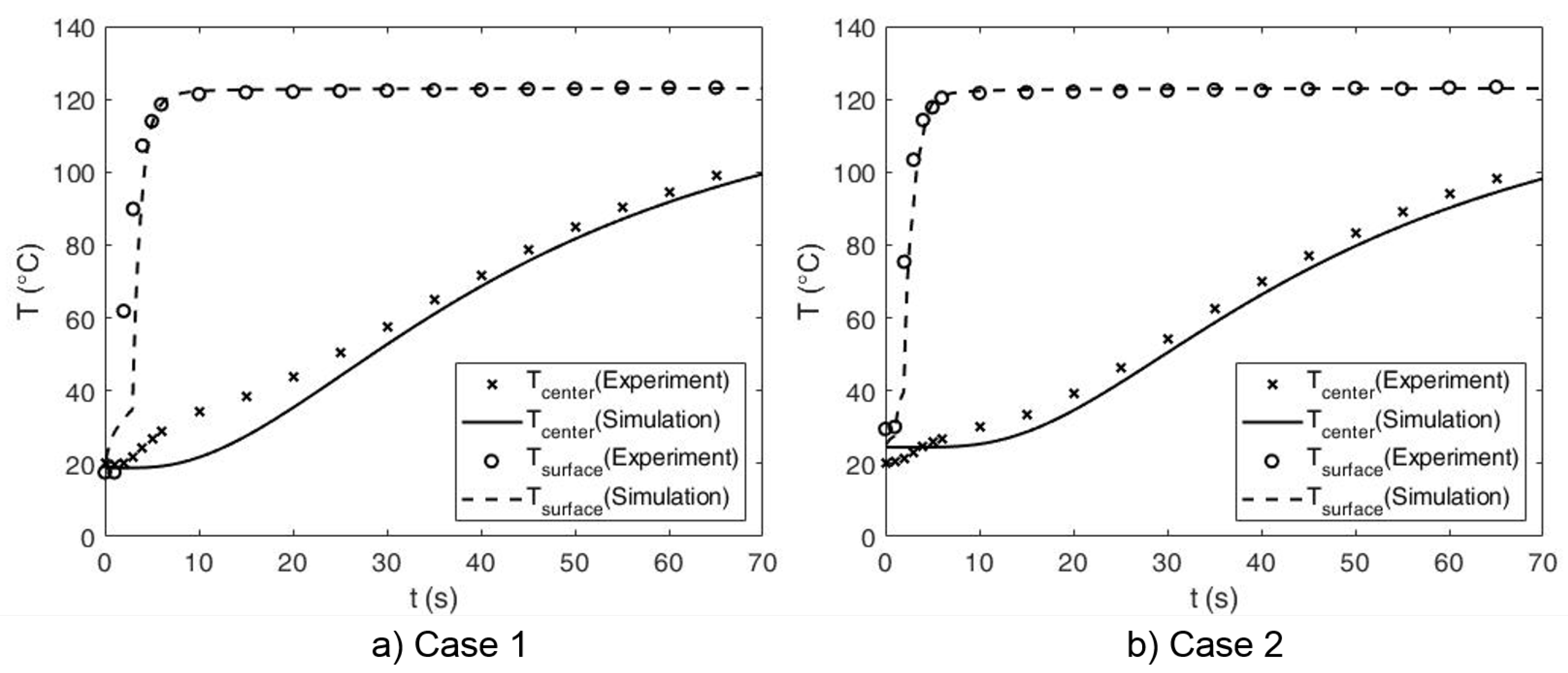
2.7. Validation of the Particle Heat Conduction Model
Before conducting a case study comparison for a complete sterilization system, we want to perform a short validation case for a heating process of a single cubic particle under almost constant fluid temperature. Heating cases of cubic potatoes in [
20] were taken for comparison with the conduction model, as discussed in
Section 2.1, which were solved using the MATLAB PDE solver. The parameters used for the heating process are summarized in
Table 1. On the one hand, the calculated surface temperature profiles agreed well with the measured values. On the other hand, the calculated center temperature values were significantly lower than the experimental values during the initial heating time, as shown in
Figure 4. Nevertheless, the discrepancy between calculated and experimental data for the center particle temperature was reduced over long heating times. Since the measurements were made based on wire-based thermocouple measurements, deviations can arise because of heat conduction and the capillary action of the hot water along the thermocouple hole and in the precise location of the measuring probe at the particle center [
21]. The model provides a realistic prediction of the particle temperature at its center and surface positions (average deviations
).
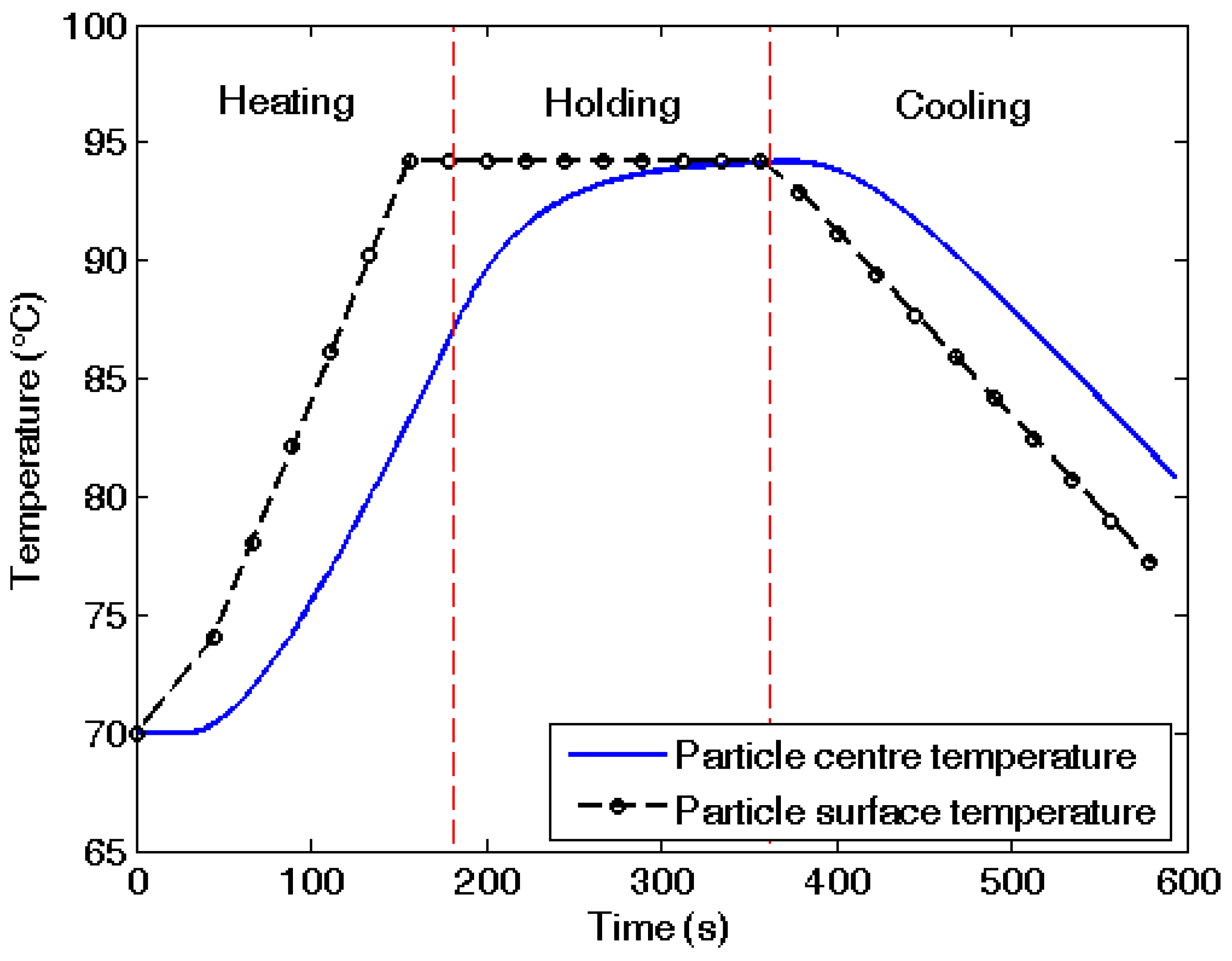
4. Result and Discussion
The particle temperature profiles in the heat exchanger, holding tube, and cooling section are plotted in
Figure 6. The particle was introduced at
m with the
value of one. The particle surface was heated in the heat exchanger (from 70
C to about 93
C), was held constant in the holding tube (at 93
C), and cooled down in the cooling section (from 93
C to approximately 76
C). The temperature of the particle center lagged behind its surface temperature. The center of the particle was heated from 70
C to approximately 86
C in the heat exchanger. In the holding tube, the center temperature rose from 86
C to the target temperature (93
C). Hence, the center of the particle reached the required temperature in the holding tube. Subsequently, the center of the particle cooled down from 93
C to approximately 82
C in the cooling section. Thus, at the exit of the cooling tube, the temperature at the center of the particle was higher than the temperature at the particle surface.
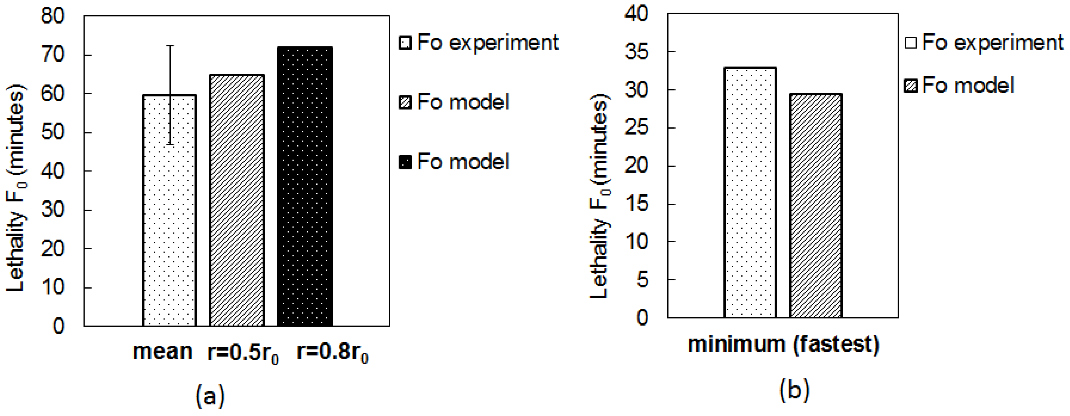
Based on the particle temperature profiles in the three sections, the
value was computed, and we made a comparison between the calculated and experimental
values for two cases. The first case was when the particle had the same residence time as the mean residence time of the product, and the second case was when the particle had the lowest residence time in the system. This also corresponded to the fastest particle flow (
). From the comparison in
Figure 7a, we observed that the simulated
values of the particle (for
and
) with the mean residence time of the products fell within the standard deviation range from the experimental mean value. In this case, we simulated the sterility values of the particle flowing at
and
, obtaining values around 65 min and 72 min, respectively. The particle traveling near the wall obtained a slightly higher
value since it was exposed to the higher fluid temperature.
As for the fastest particle, the lethality values between the experiment and model differed by around 3.5 min (approximately 10% deviation), as illustrated in
Figure 7b. A possible reason would be the following: We assumed that the fastest moving particle had a velocity two-times the mean product velocity, which is the worst-case scenario. These velocity magnitudes would not occur in reality. As determined from the experimental study in [
15], the maximum food particle velocity was around 1.8-times the mean product velocity in the holding tubes. Moreover, we assumed that the particle radial position remained the same during the process and also after passing the bends, whereas during the experiment, this may change along the tube. Further verification is required at various system parameters such as velocity, particle concentration, and particle size, such that the simplified model can be further assessed.
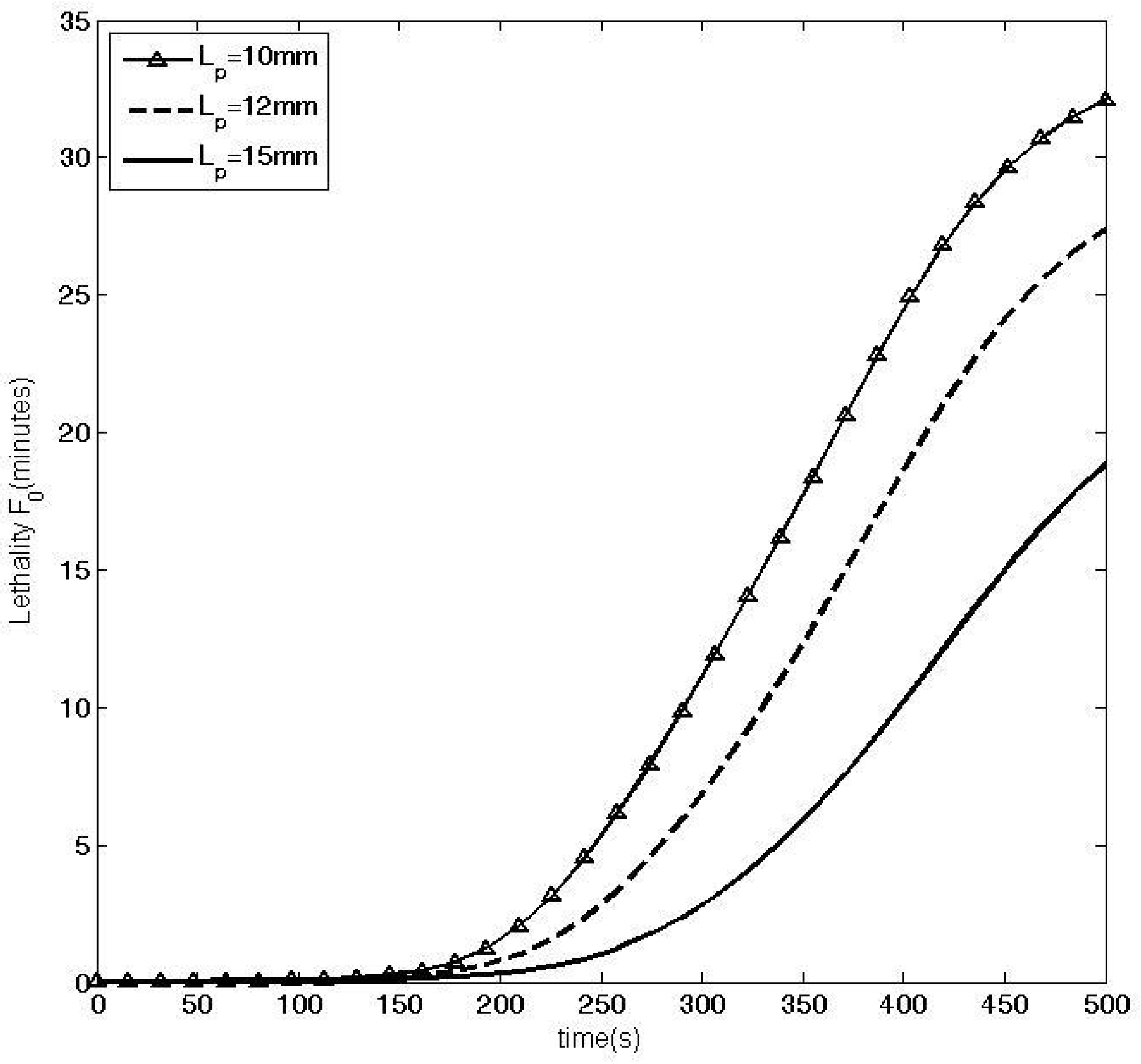
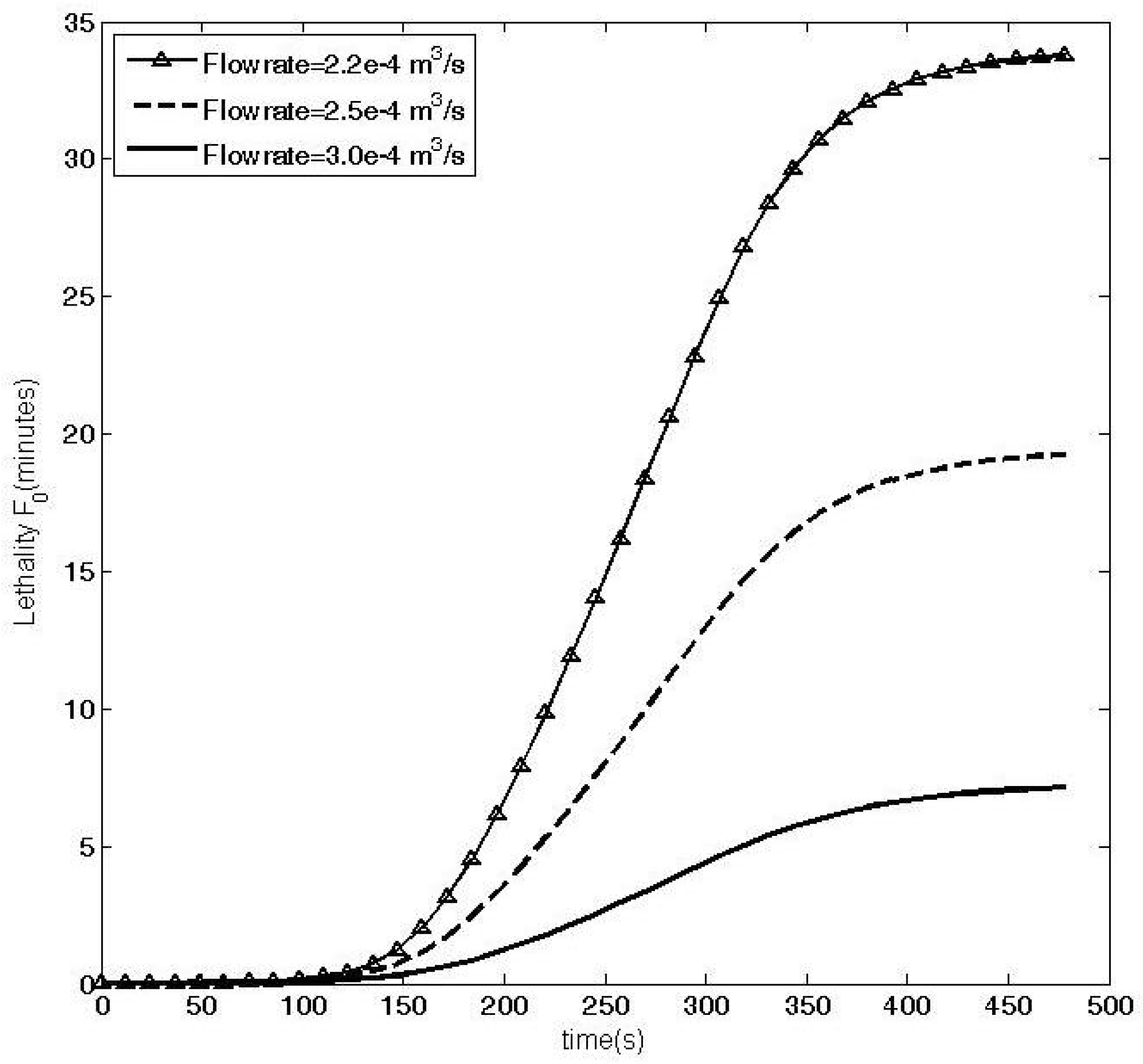
Using the modeling studies, some parameters were varied to examine the effect on the lethality values of the aseptic process. The examined parameters were the particle size, the product flow rate, the particle concentration, and the number of holding tubes in the system. The particles were introduced in the pipe at
and
, and all other parameters were kept the same as in the experimental case study from the previous section. These effects are presented graphically in
Figure 8,
Figure 9,
Figure 10 and
Figure 11. From
Figure 8, it can be seen that an increase in particle size (from 10 mm–15 mm) resulted in a decrease in the
value of the process from around 32 min to 18.8 min at
s. An increase in particle size resulted in a larger temperature gradient within the particle; hence, it took a longer time for the center of the particle to attain the required
value.
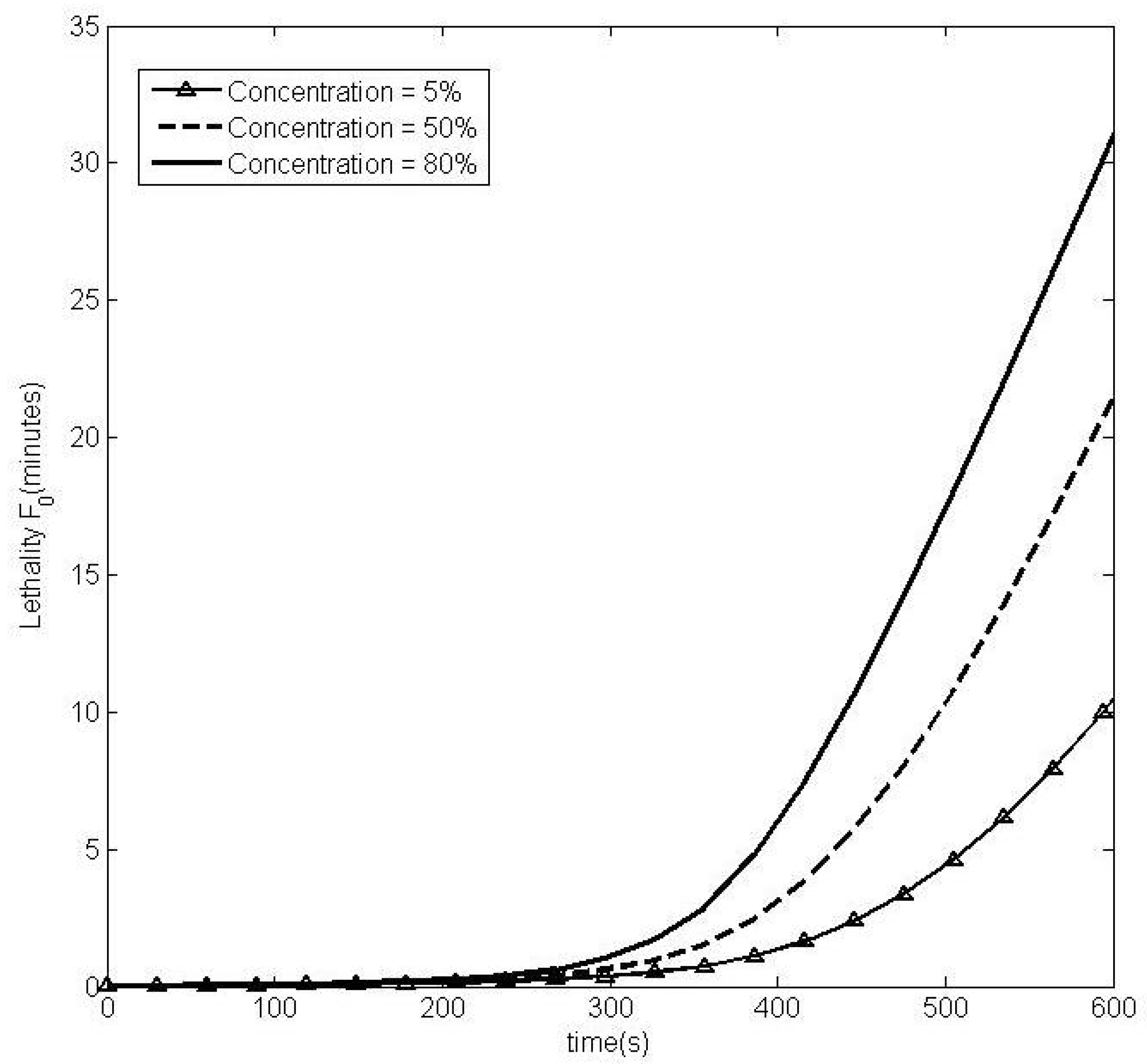
Figure 9 indicates that an increase in the particle concentration (from
–
) resulted in an increase in the
value from about 10 min to approximately 31 min at the processing time of 600 s. This may be due to the particle-particle interaction as the particle concentration increased, which led to an increase in the fluid-to-particle heat transfer coefficient. Thus, this related to a faster rate of heat transfer, and the center of the particle attained the required temperature in a shorter time (higher
value).
Figure 10 indicates that an increase in the bulk product flow rate from 2.2 m
/s–3.0 m
/s resulted in a decrease in the
value for the process from approximately 30.3 min to 6 min at
t = 350 s. A higher product bulk flow rate corresponds to a shorter residence time of the particles during the process and, hence, a lower value of
for the same length of the holding tube. The change of the system dimension was investigated (
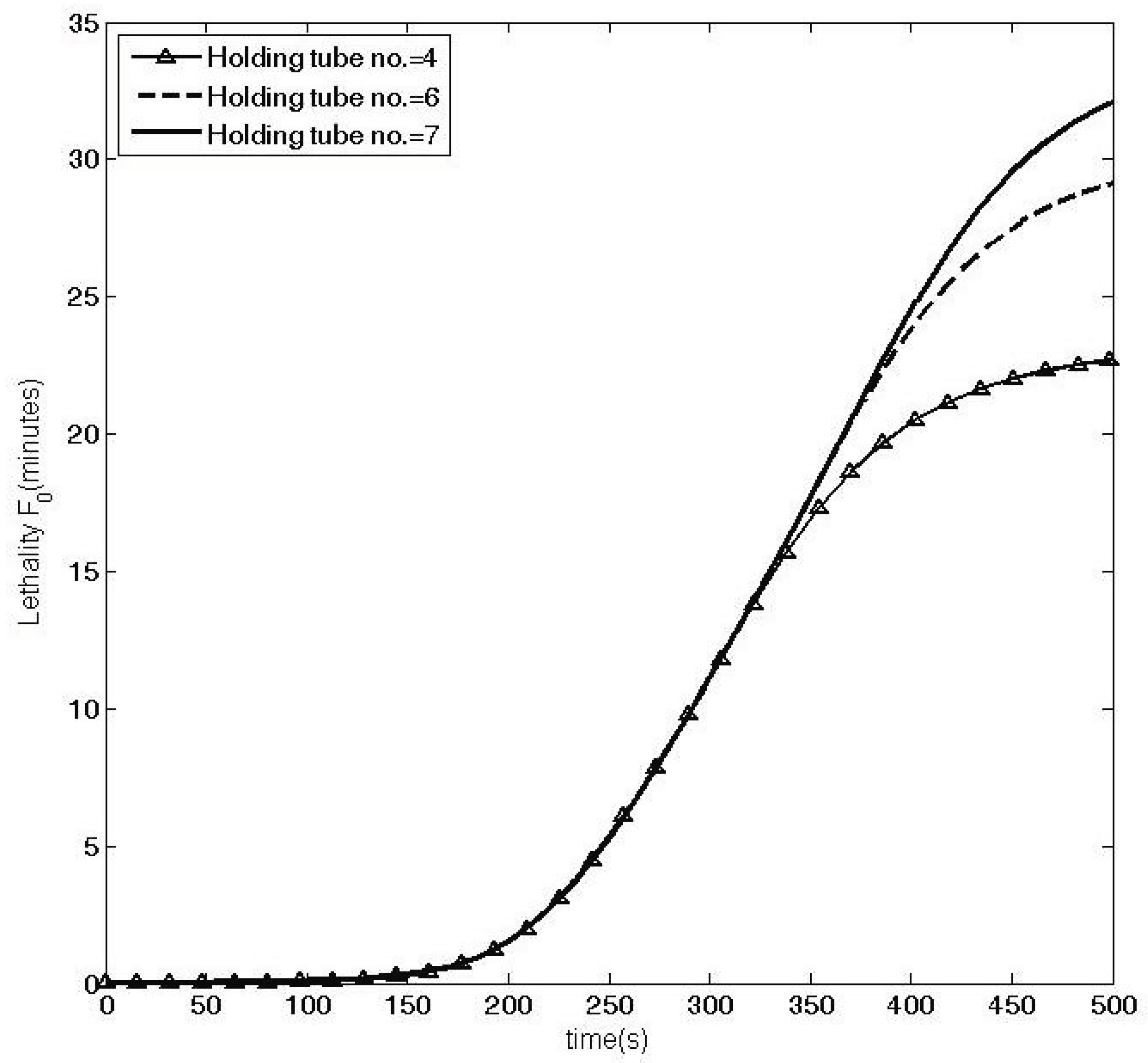
Figure 11), where a decrease of the total holding tube length translated to a decrease in the
value. Decreasing the length of the holding tube meant that the particles residence time was shorter in the holding section, as the particles were exposed to the sterilization temperature before they were cooled in the next section of the system. A minimum
value was still achieved (i.e., 6 min for this particular case from [
21]), even though the number of holding tubes was reduced from seven to four.
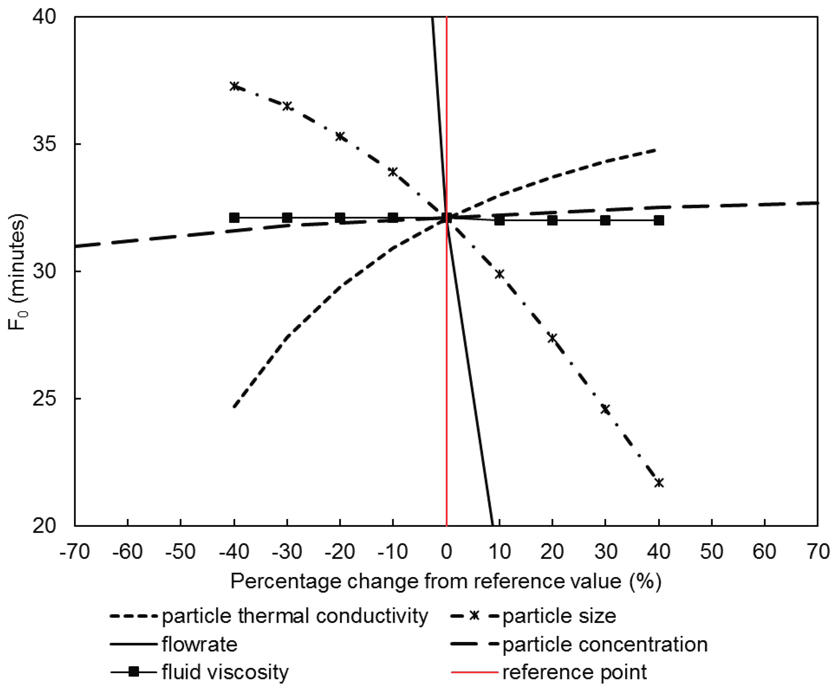
A sensitivity analysis of the simulation was conducted to evaluate the response of the model to be examined when certain changes in process parameters were made.
Figure 12 illustrates the effect of the selected parameters in
Section 3.2 on the
values at the center of the particle. The change of each parameter from the reference values was converted to a percentage change. The product flow rate had the greatest influence on the
value. Reducing the flow rate by only 3% caused a large increase in the
value, i.e., from 32.1 min to 40.0 min. This trend was observed also in the increase of the flow rate. Changes in the particle size and the particle thermal conductivity also had a significant influence on the
value; therefore, it is crucial to know the range of parameter values for raw material properties, such that one can avoid over- or under-processing. The model exhibited low sensitivity of the particle concentration on the
value, where the concentration became progressively less sensitive as the values increased from 30%–85% (−40%–70% percentage changes from the reference value, respectively). As the total simulation time to evaluate the temperature and sterilization values for each case was less than 5 min, this analysis allowed us to thoroughly perform numerous simulations using different parameter value configurations for the purposes of product and process development.
This simplified calculation algorithm for determining the temperature distribution within cubic particles and their lethality values in particular process conditions will be very useful in the food industry, as it can be implemented for preliminary designs and optimizations of aseptic processing of coarse particulate liquid foods to achieve an overall improved quality of the products. However, since several assumptions were made in this approach, it is necessary to evaluate the simulated results of temperature profiles and lethality values carefully, as they will be different from those of the complex CFD-DEM simulation approach if the same case condition and parameters are applied. The next step of this study is to compare this model with a full model of CFD-DEM simulation and sterilization experiments for verification and validation purposes.
5. Conclusions
A simplified 3D-calculation method (analytical and numerical solution) for fluid and particle temperature predictions in a system comprised of uniformly-sized cubical particles, heated in a non-mixed fluid food with time-varying temperature, was presented. The model was used to simulate the heating, holding, and cooling sections of a continuous sterilization processing unit. A number of important parameters were considered for a complete mathematical description of particulate liquid aseptic systems. Among these, the selection of appropriate calculation methods for the convective heat transfer coefficient of a Nusselt correlation at the particle surface was of particular importance in the process design. Furthermore, the position and particle residence time were required as inputs to address the heating of particles in the pipes of the sterilization process system properly.
We simulated a case study from a continuous sterilization facility experiment, and the sterilization values for two different cases were compared. This provided a good approximation for particles with the same mean residence time as the products, where the values were within the range of the mean values with the standard deviation. However, further investigation covering a wider range of parameter conditions is necessary to achieve a clearer assessment of the accuracy of this simplified model. In the modeling studies, within the considered range of parameters, the increase in flow rate and particle size resulted in a decrease of the lethality value () of the particles, whereas an increase in the particle concentration and holding tube length resulted in the opposite effect.
This model approach would be helpful for food manufacturers in the industry, since it can ascertain the impact of changes in the process and system parameters on the temperature profile or sterilization value of the products and is, hence, useful for the process design and optimization.


