Article

Adjustable Robust Optimization for Planning Logistics Operations in Downstream Oil Networks

1
CEG—IST, Instituto Superior Técnico, Universidade de Lisboa, Av. Rovisco Pais, 1049-001 Lisboa, Portugal
2
Department of Applied Mathematics, University of Málaga, 29071 Málaga, Spain
*
Author to whom correspondence should be addressed.
Processes 2019, 7(8), 507; https://doi.org/10.3390/pr7080507
Submission received: 27 April 2019 / Revised: 15 July 2019 / Accepted: 19 July 2019 / Published: 2 August 2019

Abstract

:
The oil industry operates in a very uncertain marketplace, where uncertain conditions can engender oil production fluctuations, order cancellation, transportation delays, etc. Uncertainty may arise from several sources and inexorably affect its management by interfering in the associated decision-making, increasing costs and decreasing margins. In this context, companies often must make fast and precise decisions based on inaccurate information about their operations. The development of mathematical programming techniques in order to manage oil networks under uncertainty is thus a very relevant and timely issue. This paper proposes an adjustable robust optimization approach for the optimization of the refined products distribution in a downstream oil network under uncertainty in market demands. Alternative optimization techniques are studied and employed to tackle this planning problem under uncertainty, which is also cast as a non-adjustable robust optimization problem and a stochastic programing problem. The proposed models are then employed to solve a real case study based on the Portuguese oil industry. The results show minor discrepancies in terms of network profitability and material flows between the three approaches, while the major differences are related to problem sizes and computational effort. Also, the adjustable model shows to be the most adequate one to handle the uncertain distribution problem, because it balances more satisfactorily solution quality, feasibility and computational performance.

1. Introduction

In the oil industry, companies develop a set of activities and processes so that crude oil can be duly transformed into oil products demanded by final consumers such as petrochemical industries, airports and individual users [1]. The associated decision-making process is framed within a deeply complex context and addresses the oil exploration, production and transportation at upstream, oil refining at midstream, and oil product distribution and marketing at the downstream segments [2]. Most of these activities are difficult tasks and need to be properly accomplished. Decision-support tools based on mathematical programming techniques are often applied to assist such activities and processes across the oil supply chain [3]. These optimization tools are tailored to cover the underlying reality under study, and hence they are often stochastic large-scale programs, which normally increases the problem complexity [4].
In management sciences and engineering, the most widely-used modeling framework to cope with uncertainty has been two-stage stochastic programming [2], where the first-stage variables must be decided before the uncertainty realizations and the second-stage variables are decided in accordance with the uncertainty outcomes [5]. When either the information is missing or even the probability distribution of the uncertainty is not available, fuzzy programming could be an alternative framework to handle uncertainty in optimization problems by considering random parameters as fuzzy numbers and treating constraints as fuzzy sets [6]. Robust optimization (RO) can be used, which also requires moderate information about uncertainty described by means of uncertainty sets, i.e., the key building blocks in this modeling framework [7]. Other frameworks have also been proposed to support decision making under uncertainty such as parametric programming, which relies on sensitivity analysis theory, and also chance-constrained programming, which uses probabilistic theory [8]. Currently, data-driven optimization methods are a new and timely research line to investigate the decision-making process under uncertainty, supported not only by the crescent access to uncertainty data, but also by the development in machine learning approaches [9]. Data-driven methods aims at building uncertainty sets directly from uncertainty [10]. In general, the choice of the mathematical modeling framework to solve a particular problem under uncertainty relies on the specific characteristics of this problem, as well as on the level of information about uncertainty.
The use of decision-support tools specifically for the DOSC problem under uncertainty has been a research challenge [11], and different approaches have been proposed in this direction. These include stochastic programming [1,2,4,8,12,13,14,15,16,17,18,19,20,21]; fuzzy programming [22,23]; and robust optimization [16,24]. In these optimization models, demand, supply, price, cost, process capacity, product yield, conversion rate and technology development are regarded as uncertain parameters [3].
Nowadays, RO has become attractive to solve optimization problems under uncertainty as it only requires the mean and range of the uncertain data, and other probabilistic information can be gradually incorporated when it becomes available [25]. In addition, it balances adequately solution quality, feasibility and computational performance [26], being formulated to hedge the optimization problem against any disturbances in the input data series [27]. As single-stage non-adjustable robust optimization (NARO) models may lead to over-conservative solutions [28,29,30], some authors have been emphasizing the need of exploring other methods such as the two-stage or multistage adjustable robust optimization (ARO) models, since less conservative solutions can be [28]. The first-stage and second-stage decisions are robust against all uncertain realizations of the random parameters, as well as the second-stage solution has full adaptability to the uncertainty [25].
Against this background, the purpose of this paper is to address the problem of refined products distribution under demand uncertainty in the downstream oil supply chain (DOSC). Extending previous work developed by the authors [1], where a stochastic programming approach was used considering uncertainty on price and demand for crude oil. Scenarios were built by using time series analysis. In the present work a robust modeling framework is developed that considers the problem as a two-stage adjustable robust optimization (ARO), aiming to conclude on the model conservativeness as well as on the associated solution performance. The framework includes a polyhedral uncertainty set, where the first-stage decision refers to purchase of oil volumes and the second-stage decisions include oil refining planning, oil product distribution planning, inventory management, international trade, and customer fulfillment. To evaluate the proposed model, a real-case study in the Portuguese oil industry is used. Results are compared with those obtained using the equivalent non-adjustable, stochastic and deterministic models. The robust model proposed in this paper is, to the best of the authors’ knowledge, the first model to consider an adjustable robust framework to deal with uncertainty in DOSC and, therefore, an academic contribution for this area.
The rest of the paper is structured as follows: Section 2 describes the problem under study. In Section 3, the background on two-stage ARO modeling framework is explained. Section 4 proposes the ARO mathematical formulation. In Section 5, the case study based on the Portuguese oil industry is explored. In Section 6, the obtained numerical results are discussed. Finally, Section 7 draws some conclusions and presents some directions for future research.

2. Problem Description

The problem under study consists of determining the robust tactical and operational planning of a downstream oil network under uncertainty over a planning time horizon. It must be modeled satisfactorily in a robust optimization framework so as to maximize the worst-case DOSC profit. Profit is computed as the difference between the total cost of oil purchase associated with the first-stage decisions, and the worst-case operational profit associated with the second-stage recourse decisions, in order to satisfy the uncertain product demand, subject to material balance, refining capacity, product yield, supply availability, stock limitations and transportation capacity constraints.
The network under study is composed by three echelons: oil refineries, storage depots and local markets. Crude oil is acquired by oil refineries, which process it into oil products in order to satisfy the internal and external demands. The oil products are adequately stored across the network facilities, and thus conveyed by pipelines, tanker ships, tank wagons and tank trucks from oil refineries through the primary distribution, and by tank trucks from storage depots in the secondary distribution. Oil refineries are allowed to import and export oil products, while storage depots can only import. In summary, the problem can be generally defined as follows:
Given a downstream oil system, in which an oil company manages the refining processes, storage activities, logistics, distribution, and marketing;
Determine the robust tactical and operational planning under uncertainty so as to define the production levels, yield fractions, material flows, inventory levels, demand fulfillment, transport assignment and international trade throughout the network;
Subject to material balance, product yield, equipment capacities, supply limitations, and transportation capacity constraints;
So as to maximize the worst-case network profit that comprises the worst-case recourse profit minus the total cost of crude oil procurement.
To solve this problem, a two-stage adjustable robust modeling framework, considering uncertainty in demand for refined products, is developed.

3. Two-Stage ARO Formulation

In the two-stage ARO modeling framework, the first-stage variables comprise the set of decisions that shall be made before the uncertainty is revealed and the second-stage variables include the set of decisions that must be made after the uncertainty is disclosed. The second-stage decision variables have fully adaptability to any realization of the uncertainty [25]. Considering a linear formulation and let x and y be the corresponding first-stage and second-stage decision variables, while U is either a polyhedral or a discrete uncertainty set, according to Zeng and Zhao [28], the general form of a two-stage ARO formulation can be defined as follows:
max x c T x + min u U max y F ( x , u ) b T y
s . t . A x d , x S x
where F ( x , u ) = { y S y : G y h E x M u } with S x + n and S y + m . If the uncertainty set U is continuous, the optimization problem (Equations (1) and (2)) will have an infinite number of constraints in the second-stage problem [27]. However, when U is a polyhedral uncertainty set, only its extreme points, i.e., its vertices, might belong to an optimal solution of that second-stage problem [25]. In accordance with Zeng and Zhao [28], when considering only a finite and discrete set of extreme points U = { u 1 , , u r } , as well as the set of the respective recourse decision variables { y 1 , , y r } , the prior optimization problem can be recast as presented below:
max x c T x + η
s . t . A x d
η b T y v , v = 1 , ,
E x + G y v h M u v , v = 1 , , r
x S x , y v S y , v = 1 , , r .
consequently, we can find a solution for the two-stage ARO model (Equations (1) and (2)) through solving its mixed-integer linear program counterpart (Equations (3)–(7)). However, defining this equivalent formulation and determining its solution can often be difficult and dependent on the size of the finite and discrete uncertainty set U = { u 1 , , u r } [28].

4. Adjustable Robust Mathematical Programming Model

Having defined in a generic form the two-stage ARO approach, the tactical and operational planning for the DOSC is now considered, which aims at maximizing the worst-case network profit under refined product uncertainty. In the established two-stage ARO problem, the first-stage decisions, i.e., the here-and-now decisions, comprise the crude oil purchase, while the second-stage decisions, i.e., the recourse (wait-and-see) decisions, include production levels, product yields, material flows, inventory levels, demand fulfillment, transport allocation and international trade, which are made in accordance with the realization of the product demand uncertainty. The two-stage ARO model for the general distribution problem under uncertain demand for refined products is formulated hereinafter.

4.1. Robust Objective Function

The notation used to formulate the two-stage ARO model is outlined in Table A1 of Appendix A. As shown in Equation (8), the objective function aims at maximizing the worst-case network profit (WCP), which can be stated as follows:
max X C O W C P = i I , t T X C O i , t P O t + Q U ( X C O )
s . t . X C O i , t D O i , t i I , t T
where X C O i , t represents the crude oil purchase at oil refinery i in time point t and refers to the first-stage decisions. Q U ( · ) is defined as a function of the first-stage (here-and-now) decisions and denotes the worst-case recourse profit, which must be determined for the worst-case scenario of the uncertain product demands in the second-stage problem. Here, uncertainty is modeled through a polyhedral uncertainty set U , where the uncertain parameters can take values in, because such fact guides to define a robust counterpart that corresponds to a linear programming problem [27]. Equation (9) limits the amount of crude oil purchased by each oil refinery i at time point t by the corresponding oil demand.
The worst-case recourse profit Q U ( · ) is equal to the objective function value of the next robust formulation, Equation (10), which can be formulated as follows:
Q U ( · ) = min Δ D P k , p , t U max ( , Δ D P k , p , t ) ( i I , t T R R i , t + j J , p P , t T M D j , p , t + k K , p P , t T M C k , p , t i I , p P , t T C E i , p , t h H , p P , t T C I h , p , t i I , p P , t T C P D i , p , t j J , p P , t T C S D j , p , t i I , t T C I O i , t i I , p P , t T C I R i , p , t j J , p P , t T C I D j , p , t k K , p P , t T C I M k , p , t k K , p P , t T C U D k , p , t )
where U represents the polyhedral uncertainty set that is used to describe the stochastic parameters, + denotes the set of recourse decisions, i.e., = {XR,XOP,XCO,XP,XS,XRP,XU,XE,XI,IO,IR,ID,IM}, + depicts the set of here-and-now decisions, = { X C O } , and is a set defined as a function of the set of here-and-now decisions and the worst-case realization of the deviations Δ D P k , p , t from the nominal values D P ^ k , p , t . Notice that the set of recourse decisions is made after the outer minimization problem selects the worst-case realization of the deviations of the product demands Δ D P k , p , t . In other words, the m i n - m a x problem picks the worst realization of the demand that minimizes the network profit. Therefore, the robust modeling framework concerns with the maximization of the recourse profit in the worst-case scenario of the random parameter within the uncertainty set U . In summary, the two-stage RO model addresses the volumes of exported and imported products, refined oil, product yield fractions, primary and secondary product distributions, inventories of oil and products, and met and unmet demand as the second-stage decisions, which are adjusted to the volumes of purchased oil, i.e., the first-stage decisions, after uncertainty is disclosed.
The worst-case recourse profit Q U ( · ) , i.e., Equation (10), includes the revenues from the sales of refined products by the oil refineries, margins from buying and selling refined products by the storage depots and local markets, and costs for exporting, importing, transporting, and storing refined products throughout the network. Before presenting the equations of the recourse optimization problem Q U ( · ) , the associated revenues, margins and costs are now discussed, being outlined by the set of Equations (11)–(22) below:
R R i , t = p P [ X R i , p , t × ( P P a , p , t T N r , p ) ] i I , t T , a = r = = r e f i n e r y
M D j , p , t = ( k , m ) R o u t e i , j , m X S j , k , m , p , t × ( P P a , p , t T N r , p ) ( i , m ) R o u t e i , j , m X P i , j , m , p , t × P P a 2 , p , t
j J , p P , t T , a = r = d e p o t , a 2 = r e f i n e r y
M C k , p , t = [ ( X R P k , p , t X U k , p , t ) × ( P P a 1 , p , t T N r , p ) ] [ ( ( i , m ) R o u t e i , k , m X P i , k , m , p , t ) × P P a 2 , p , t + ( ( j , m ) R o u t e j , k , m X S j , k , m , p , t ) × P P a 3 , p , t ]
k K , p P , t T , a 1 = r = r e t a i l , a 2 = r e f i n e r y , a 3 = d e p o t
C E i , p , t = X E i , p , t × T N r , p i I , p P , t T , r = e x p o r t
C I h , p , t = X I h , p , t × ( P P a , p + T N r , p ) h H , p P , t T , a = r = i m p o r t
C P D i , p , t = ( l , m ) R o u t e i , l , m ( X P i , l , m , p , t × C T m , p × D i s t i , l , m ) i I , p P , t T
C S D j , p , t = ( k , m ) R o u t e j , k , m ( X S j , k , m , p , t × C T m , p × D i s t j , k , m ) j J , p P , t T
C I O i , t = C K I × I O i , t × P O t i I , t T , p = o i l
C I R i , p , t = C K I × I R i , p , t × P P a , p , t i I , p P , t T , a = r e f i n e r y
C I D j , p , t = C K I × I D j , p , t × P P a , p , t j J , p P , t T , a = d e p o t
C I M k , p , t = C K I × I M k , p , t × P P a , p , t k K , p P , t T , a = r e t a i l
C U D k , p , t = X U k , p , t × T N r , p k K , p P , t T , r = u n m e t
Equation (11) defines the refinery revenues obtained from the sales of refined products. Equations (12) and (13) determine the storage depot margins and the local market margins, respectively, being the difference between the revenues from selling refined products and the costs for buying these ones. Equations (14) and (15) specify, respectively, the costs of exporting and importing refined products. Equations (16) and (17) determine the costs for dispatching refined products through the primary and secondary distributions, in that order. Equation (18) defines the crude oil inventory costs at oil refineries, whereas Equations (19)–(21) define, respectively, the refined product inventory costs at oil refineries, storage depots and local markets. Equation (22) represents the costs for not supplying the required product demand.

4.2. Equations of the Recourse Problem Q U ( · )

Equations (23)–(45) of the second-stage problem Q U ( · ) depend on the worst-case realization of the stochastic parameters and are used to model the refinery operation, network flow allocation, inventory policy, and so on:
X O P i , t P C i i I , t T
X R i , p , t = X O P i , t × Y F i , p i I , p P , t T
I O i , t = I S O i + X C O i , t X O P i , t i I , t T , t = t 1
I O i , t = I O i , t 1 + X C O i , t X O P i , t i I , t T , t > t 1
I R i , p , t = I S P i , p + X R i , p , t + X I i , p , t ( l , m ) R o u t e i , l , m X P i , l , m , p , t X E i , p , t
i I , p P , t T , t = t 1
I R i , p , t = I R i , p , t 1 + X R i , p , t + X I i , p , t ( l , m ) R o u t e i , l , m X P i , l , m , p , t X E i , p , t
i I , p P , t T , t > t 1
I D j , p , t = I S P j , p + X I j , p , t + ( i , m ) R o u t e i , j , m X P i , j , m , p , t ( k , m ) R o u t e j , k , m X S j , k , m , p , t
j J , p P , t T , t = t 1
I D j , p , t = I D j , p , t 1 + X I j , p , t + ( i , m ) R o u t e i , j , m X P i , j , m , p , t ( k , m ) R o u t e j , k , m X S j , k , m , p , t
j J , p P , t T , t > t 1
I M k , p , t = I S P k , p + ( i , m ) R o u t e i , k , m X P i , k , m , p , t + ( j , m ) R o u t e j , k , m X S j , k , m , p , t + X U k , p , t X R P k , p , t + Δ D P k , p , t
k K , p P , t T , t = t 1
I M k , p , t = I M k , p , t 1 + ( i , m ) R o u t e i , k , m X P i , k , m , p , t + ( j , m ) R o u t e j , k , m X S j , k , m , p , t + X U k , p , t X R P k , p , t + Δ D P k , p , t
k K , p P , t T , t > t 1
X R P k , p , t ( D P ^ k , p , t + Δ D P k , p , t ) k K , p P , t T
S S O i × S C O i I O i , t S C O i i I , t T
S S P i × S C i , p I R i , p , t S C i , p i I , p P , t T
S S P j × S C j , p I D j , p , t S C j , p j J , p P , t T
S S P k × S C k , p I M k , p , t S C k , p k K , p P , t T
l R o u t e i , l , m X P i , l , m , p , t A S P D i , m , p i I , m M , p P , t T
k R o u t e j , k , m X S j , k , m , p , t A S S D j , m , p j J , m M , p P , t T
p P X P i , l , m , p , t A C P D i , l , m ( i , l , m ) R o u t e i , l , m , t T
p P X S j , k , m , p , t A C S D j , k , m ( j , k , m ) R o u t e j , k , m , t T
( i , m ) R o u t e i , j , m X P i , j , m , p , t + X I j , p , t S C j , p × T C M j , p j J , p P , t T
( i , m ) R o u t e i , k , m X P i , k , m , p , t + ( j , m ) R o u t e j , k , m X S j , k , m , p , t S C k , p × T C M k , p k K , p P , t T
X P i , l , m , p , t = 0 i I , l L , p P , t T , m = r o a d , μ i , j , m > M T D
X S j , k , m , p , t = 0 j J , k K , p P , t T , m = r o a d , μ j , k , m > M T D
Equation (23) limits the oil processed at oil refineries. Equation (24) defines the fractions obtained through the crude oil distillation process. Equations (25) and (26) control the crude oil balance, as well as Equations (27) and (28) handle the refined product balance, at oil refineries. Likewise, Equations (29) and (30) control the refined product balance at storage depots, as well as Equations (31) and (32) do it at local markets. Equation (33) limits the product supply at local markets by the nominal product demand plus the associated deviation. Equations (34)–(37) determine the storage capacities for the facilities in the network. Equation (38) limits the capacity of supplying refined products in the primary distribution, as well as Equation (39) does so in the secondary distribution. Equation (40) defines the arc capacities for the primary distribution, whereas Equation (41) for the secondary distribution. Equations (42) and (43) determine the receiving capacities for the storage depots and local markets, respectively. Equation (44) and (45) suppress the primary and secondary distributions for long distances, respectively.

4.3. Definition of Uncertainty Set U

The uncertainty set is the key building block of the robust modeling framework [7]. It is assumed that the deviation of the product demand Δ D P k , p , t takes values within a convex and budget uncertainty set (Equations (46)–(48)) as follows—see [31]:
Δ D P k , p , t = D P ˜ k , p , t D P ^ k , p , t k K , p P , t T
| Δ D P k , p , t | Δ D P k , p , t m a x k K , p P , t T
t | Δ D P k , p , t | Δ D P k , p , t m a x Γ k , p k K , p P
Equation (46) defines the demand deviation Δ D P k , p , t as the difference between the uncertain value of the product demand D P ˜ k , p , t and the nominal value of the demand D P ^ k , p , t . Equation (47) models the symmetrical and bounded range for the deviations of the product demand Δ D P k , p , t . Equation (48) ensures that the sum of the normalized absolute values of the demand deviations for each pair of location and product, across all time points t , must not exceed the user-defined budget of uncertainty Γ k , p . Notice that the normalized absolute value corresponds to the quotient between the absolute and maximum values of the demand deviation, while the uncertain value of the product demand refers to the unknown realization of the product demand. Appendix E includes an example showing how to define the vertices of a polyhedral budget uncertainty set.

4.4. The Adaptive Robust Formulation
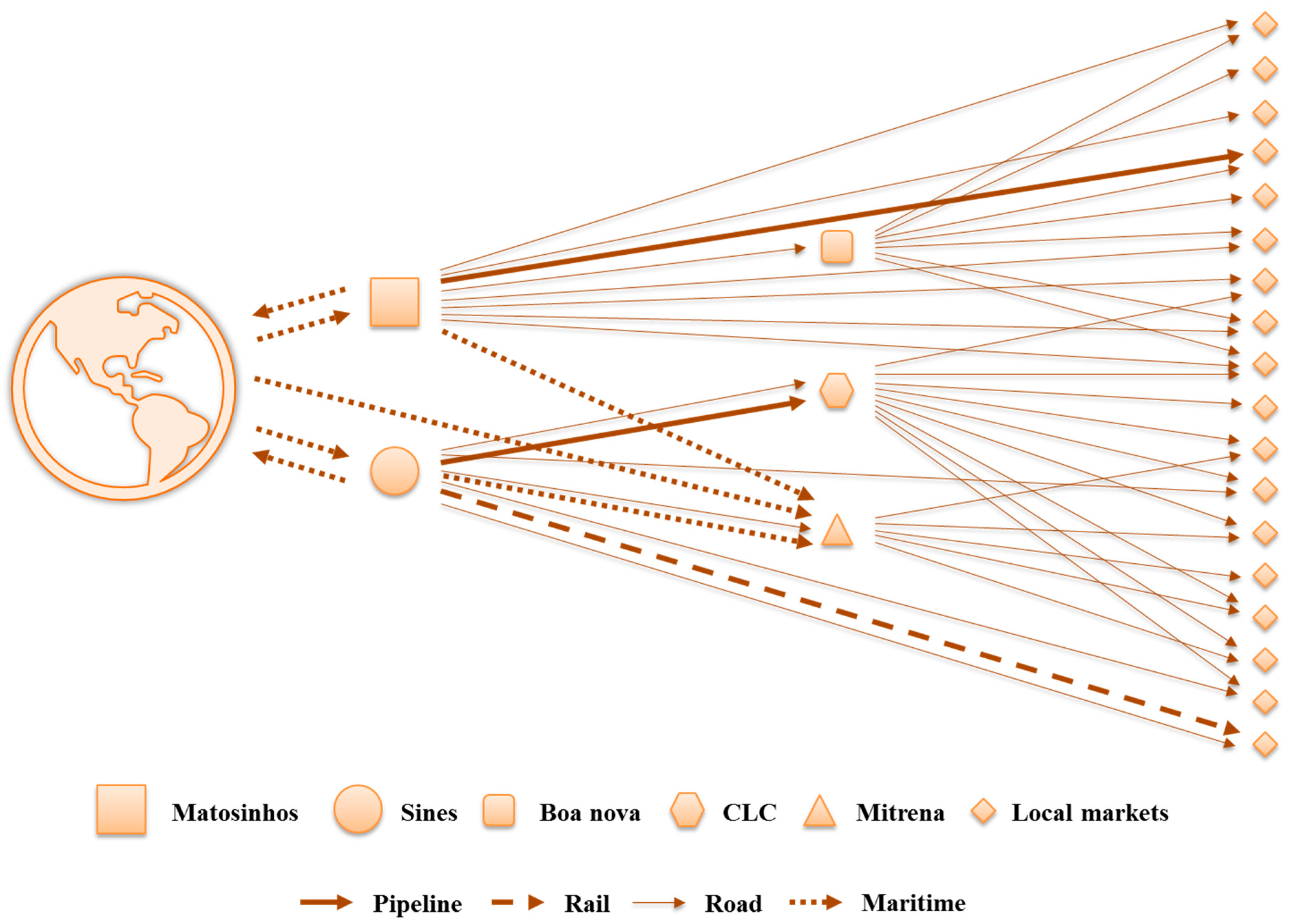
In this section, the above robust formulation, that is, the set of Equations (8)–(48), is reformulated to be fully adaptive to the realizations of the uncertain deviations of the product demands Δ D P k , p , t . In order to transform the prior robust formulation into a single-level approach, the worst-case recourse profit Q U ( · ) may be denoted by an auxiliary variable α , which must be lower or equal to the difference among the financial items—see Equation (49). Moreover, the set of recourse decisions of the second-stage problem Q U ( · ) is reformulated as a function of the uncertain deviations of the product demands Δ D P k , p , t , which are defined by the uncertainty set U (Equations (46)–(48)). Because this uncertainty set U defines a polyhedron with infinite number of points, this reformulation would result in a recourse problem with an infinite number of variables and equations. For this reason, the uncertainty set U must be partitioned into K parts in order to make the resulting formulation tractable. According to Bertsimas et al. [25], only an extreme point (i.e., a vertex) of the defined polyhedron can be part of the optimal solution of the recourse problem Q U ( · ) . Hence, only the set of vertices v V of the polyhedron defined through the uncertainty set U is considered in this adjustable robust formulation. Therefore, the adjustable robust formulation is defined in the following set of Equations (49)–(86):
max , , α W C P = i I , t T X C O i , t × P O t + α
s . t . X C O i , t D O i , t i I , t T
α min Δ D P k , p , t U max ( , Δ D P k , p , t max ) ( i I , t T R R i , t , v + j J , p P , t T M D j , p , t , v + k K , p P , t T M C k , p , t , v i I , p P , t T C E i , p , t , v h H , p P , t T C I h , p , t , v i I , p P , t T C P D i , p , t , v j J , p P , t T C S D j , p , t , v i I , t T C I O i , t , v i I , p P , t T C I R i , p , t , v j J , p P , t T C I D j , p , t , v k K , p P , t T C I M k , p , t , v k K , p P , t T C U D k , p , t , v )
v V
R R i , t , v = p P [ X R i , p , t , v × ( P P a , p , t T N r , p ) ] i I , t T , v V , a = r = r e f i n e r y
M D j , p , t , v = ( k , m ) R o u t e i , j , m X S j , k , m , p , t , v × ( P P a , p , t T N r , p ) ( i , m ) R o u t e i , j , m X P i , j , m , p , t , v × P P a 2 , p , t
j J , p P , t T , v V , a = r = d e p o t , a 2 = r e f i n e r y
M L k , p , t , v = [ ( X R P k , p , t , v X U k , p , t , v ) × ( P P a 1 , p , t T N r , p ) ] [ ( ( i , m ) R o u t e i , k , m X P i , k , m , p , t , v ) × P P a 2 , p , t + ( ( j , m ) R o u t e j , k , m X S j , k , m , p , t , v ) × P P a 3 , p , t ]
k K , p P , t T , v V , a 1 = r = r e t a i l , a 2 = r e f i n e r y , a 3 = d e p o t
C E i , p , t , v = X E i , p , t , v × T N r , p i I , p P , t T , v V , r = e x p o r t
C I h , p , t , v = X I h , p , t , v × ( P P a , p + T N r , p ) h H , p P , t T , v V , a = r = i m p o r t
C P D i , p , t , v = ( l , m ) R o u t e i , l , m ( X P i , l , m , p , t , v × C T m , p × D i s t i , l , m ) i I , p P , t T , v V
C S D j , p , t , v = ( k , m ) R o u t e j , k , m ( X S j , k , m , p , t , v × C T m , p × D i s t j , k , m ) j J , p P , t T , v V
C I O i , t , v = C K I × I O i , t , v × P O t i I , t T , v V , p = o i l
C I R i , p , t , v = C K I × I R i , p , t , v × P P a , p , t i I , p P , t T , v V , a = r e f i n e r y
C I D j , p , t , v = C K I × I D j , p , t , v × P P a , p , t j J , p P , t T , v V , a = d e p o t
C I M k , p , t , v = C K I × I M k , p , t , v × P P a , p , t k K , p P , t T , v V , a = r e t a i l
C U D k , p , t , v = X U k , p , t , v × T N r , p k K , p P , t T , v V , r = u n m e t
X O P i , t , v P C i i I , t T , v V
X R i , p , t , v = X O P i , t , v × Y F i , p i I , p P , t T , v V
I O i , t , v = I S O i + X C O i , t X O P i , t , v i I , v V , t T , t = t 1
I O i , t , v = I O i , t 1 , v + X C O i , t X O P i , t , v i I , v V , t T , t > t 1
I R i , p , t , v = I S P i , p + X R i , p , t , v + X I i , p , t , v ( l , m ) R o u t e i , l , m X P i , l , m , p , t , v X E i , p , t , v
i I , p P , v V , t T , t = t 1
I R i , p , t , v = I R i , p , t 1 , v + X R i , p , t , v + X I i , p , t , v ( l , m ) R o u t e i , l , m X P i , l , m , p , t , v X E i , p , t , v
i I , p P , v V , t T , t > t 1
I D j , p , t , v = I S P j , p + X I j , p , t , v + ( i , m ) R o u t e i , j , m X P i , j , m , p , t , v ( k , m ) R o u t e j , k , m X S j , k , m , p , t , v
j J , p P , v V , t T , t = t 1
I D j , p , t , v = I D j , p , t 1 , v + X I j , p , t , v + ( i , m ) R o u t e i , j , m X P i , j , m , p , t , v ( k , m ) R o u t e j , k , m X S j , k , m , p , t , v
j J , p P , v V , t T , t > t 1
I M k , p , t , v = I M k , p , t 1 , v + ( i , m ) R o u t e i , k , m X P i , k , m , p , t , v + ( j , m ) R o u t e j , k , m X S j , k , m , p , t , v + X U k , p , t , v X R P k , p , t , v + Δ D P k , p , t , v
k K , p P , v V , t T , t > t 1
X R P k , p , t , v ( D P ^ k , p , t , v + Δ D P k , p , t , v ) k K , p P , t T , v V
S S O i × S C O i I O i , t , v S C O i i I , t T , v V
S S P i × S C i , p I R i , p , t , v S C i , p i I , p P , t T , v V
S S P j × S C j , p I D j , p , t , v S C j , p j J , p P , t T , v V
S S P k × S C k , p I M k , p , t , v S C k , p k K , p P , t T , v V
l R o u t e i , l , m X P i , l , m , p , t , v A S P D i , m , p i I , m M , p P , t T , v V
k R o u t e j , k , m X S j , k , m , p , t , v A S S D j , m , p j J , m M , p P , t T , v V
p P X P i , l , m , p , t , v A C P D i , l , m ( i , l , m ) R o u t e i , l , m , t T , v V
p P X S j , k , m , p , t , v A C S D j , k , m ( j , k , m ) R o u t e j , k , m , t T , v V
( i , m ) R o u t e i , j , m X P i , j , m , p , t , v + X I j , p , t , v S C j , p × T C M j , p j J , p P , t T , v V
( i , m ) R o u t e i , k , m X P i , k , m , p , t , v + ( j , m ) R o u t e j , k , m X S j , k , m , p , t , v S C k , p × T C M k , p k K , p P , t T , v V
X P i , l , m , p , t , v = 0 i I , l L , p P , t T , v V , m = r o a d , μ i , j , m > M T D
X S j , k , m , p , t , v = 0 j J , k K , p P , t T , v V , m = r o a d , μ j , k , m > M T D

5. Case Study

The ARO model is applied to a real case study on a refined products network distribution in the Portuguese oil industry, which was originally characterized by Lima et al. [1]. Figure 1 represents the network under study.
The network comprises two oil refineries (Sines and Matosinhos), three distribution centers (Boa nova, CLC and Mitrena), 278 local markets (Portuguese cities) and four transportation modes (pipeline transport, railway, roadway and waterway). In this network, the oil refineries import the same type of crude oil and produce eight refined products, namely, jet fuel, diesel, propane, butane, fuel oil, gas oil, gasoline 95 and gasoline 98. These refined products are then transported using pipelines, tanker ships, tank wagons and tank trucks from the oil refineries, and using only tank trucks from the distribution centers. Roadway is only considered for distances less than or equal to 250 km. The planning horizon considered is 6 months, which is discretized into monthly cycles. For the sake of comparison, the same database employed by Lima et al. [1] is used in the case study.

6. Results and Discussion

The proposed two-stage ARO model is implemented in GAMS 24.5.6 and solved using CPLEX 12.6 on an Intel(R) Xeon(R) processor CPU E5-2660 v3 @ with 2.60 GHz (two processors) and 64 GB RAM memory.

6.1. Setup of the ARO Model

In the practical application, the ARO model was run under a specific configuration of the budget uncertainty set (Equations (46)–(48)). In other words, the ARO model was solved after specifying the parameters of the polyhedral uncertainty set, namely, the nominal value D P ^ k , p , t and the maximum deviation in absolute value Δ D P k , p , t m a x of the uncertain product demand D P ˜ k , p , t , besides the budget of uncertainty Γ k , p . The values of these parameters were estimated from the dataset described by Lima et al. [1]. Therefore, the maximum deviation Δ D P k , p , t m a x was estimated as 10% of the nominal value D P ^ k , p , t , while the budget of uncertainty Γ k , p was set to the average of the total relative deviations over the time horizon for the pairs of local market and product. To be more precise, for each pair of location and product ( k , p ) , the absolute value of the product demand deviation Δ D P k , p , t is normalized to the associated maximum deviation Δ D P k , p , t m a x at each time point. We then sum of all the so normalized deviations over the time horizon. Finally, we average these normalized values over all pairs of products and locations, and the result (let’s denote it by Γ ^ k , p ) is considered as the value of the budget of uncertainty, that is, Γ ^ k , p for all ( k , p ) . This results in Γ ^ k , p = 0.895 , for all ( k , p ) , which leads to uncertainty sets (i.e., Equations (46)–(48)) consisting in polyhedrons of 12 vertices.

6.2. Comparison with the Developed Approaches

In this section, we compare the results given by the proposed adjustable robust optimization (ARO) model with those obtained using the equivalent non-adjustable robust optimization (NARO), stochastic programming (SP) and the deterministic (DM) models. The mathematical formulations, the model notations and the specific settings for the DM, NARO and SP models can be found in Appendix B, Appendix C, Appendix D, respectively.

6.2.1. Computational Performance

Table 1 presents the problem size, economic performance and solving time for all the optimization models.
From Table 1, we can conclude that the economic performance (i.e., the profit) declines when uncertainty in demand for refined products is taken into consideration by the optimization model. On the other hand, a model in which all the parameters are considered as deterministic (DM) is not realistic, and it should consider random parameters to provide robustness and consistency to the decision maker.
In this way, the SP model aims at maximizing the expected profit for a set of scenarios, while the robust approaches maximize the total profit of the worst-case scenario. Compared to the ARO approach, the profit is higher about 0.16% for the SP approach. When comparing both robust approaches, the ARO model shows a better economic performance, providing a profit that is almost 0.80% higher than the one returned by the NARO model, which is the most conservative approach.
The problem size is also different for all the considered formulations. That is, the size of the deterministic model is smaller than the other methods, and thus it requires less computational time (1.484 CPU seconds). The NARO model does not increase too much the problem size and the computational time, because its size raises as more dual variables and robust constraints are incorporated into the problem, and such an increase is at the same scale as the number of the added random parameters, which in this case is only the demand for refined products. Nevertheless, much more computational burden is demanded to solve the much bigger ARO and SP models (95.3 and 236.8 CPU seconds, respectively). The size of the ARO model relies on the size of the polyhedral uncertainty set (Equations (46)–(48)), which in turn is determined by the budget of uncertainty Γ k , p in Equation (48). The size of the scenario-based SP model depends on the number of the considered scenarios, which in this case amounts to 243, in order to model the uncertainty in the stochastic parameter. All in all, the ARO approach does not increase the problem size as much as the SP approach when compared with the nominal problem (i.e., DM), having better solution performance, while it approximates better the economic result of the SP when comparing to the NARO approach.

6.2.2. Insights about the Network Profitability

The contribution of the different activities to the network profitability is illustrated in Figure 2 for all the optimization models. The oil procurement costs and the refinery revenues are all included into the margins of the refinery sector, so that the comparisons can be possible with the margins of the distribution and market sectors. In general, the profit breakdown is not too affected when the case study is solved by the different models. As the only difference in these approaches is how uncertainty is modeled, the reason comes from that. Firstly, the same uncertainty set U is considered by both robust optimization approaches. Secondly, the stochastic approach provides an average result of the considered scenarios, which are properly defined in accordance with the level of uncertainty considered by the robust approaches. Lastly, the product demand uncertainty does not actually interfere too much in the profit breakdown.
As it can be seen in Figure 2, the market sector delivers the largest contribution to the network profitability, followed by the refining and distribution sectors, respectively. When comparing both robust approaches, the profit breakdown differs. The NARO model increases the shares of the refining and market sectors and decreases the contribution of the distribution sector when compared with the ARO model. The SP and DM models result in the same profit breakdown, which is slightly different from the one determined by the ARO model, where the market contribution rises 1% and the distribution sector diminishes 1%, whereas the share of the refining sector remains unaltered.
Figure 3 compares the effective profitability contribution of the network sectors among the different optimization models. All the optimization approaches provide quite similar results for the refining sector. The same fact is not observed in the distribution and market sectors, where the NARO model returns the lowest economic performance. These facts corroborate that the NARO model is the most conservative approach to handle uncertainty in this case study.
In order to get more insights about the network profitability, the cost breakdown information is also investigated. As abovementioned, refinery margins comprise the revenues for selling oil products and the cost for acquiring crude oil. The oil procurement cost is the major cost item, and accounts for at least 78.53% of the overall cost in all the developed approaches, while the other costs together account for at most 21.47% of the same total. The oil procurement cost amounts to 78.53%, 80.92%, 78.94% and 78.54% of the total network cost in the ARO, NARO, SP and DM approaches, respectively. The cost breakdown information of the studied models is illustrated in Figure 4. Even though the exportation and lost demand costs are included in the estimation of the cost breakdown, their slices of the overall cost are quite small, i.e., almost 0%, and hence they have been omitted to enhance the readability of the charts without loss of generality.
As shown in Figure 4, the total network cost is divided into the same proportions for both ARO and DM approaches, while the proportions are much different for the other approaches. For instance, the SP and NARO approaches have increased the oil procurement cost by 1% and 3%, respectively, and have decreased the total of the other costs by 1% and 3%, respectively, when compared with the previous approaches. In most cases, the importation cost is the second most relevant cost item, followed by the secondary and primary transportation costs, respectively. The inventory cost aggregates the costs for keeping inventories of oil and refined products at the network facilities and amounts to 1% of the overall cost.
Figure 5 compares the absolute values of the cost items among the optimization methods. Notice that the oil procurement cost is not displayed, because it is much larger than the other cost items, and assumes quite similar values in all the methods, i.e., €2,408,811,163 on average. As it can be seen in Figure 5, the ARO and DM methods have much similar network costs, which are usually higher than the cost items for the NARO and SP models. Notice that the export and unmet demand costs are much smaller than the other cost items, and hence they are displayed in a different scale. Even though the NARO presents the best performance with regards to the network costs, its poorer performance in the network margins makes it as the most conservative approach. In turn, the SP model is the less conservative model, but it is not so efficient as the others in order to fulfill the required demand, and thus the lost demand is larger.

6.2.3. Network Planning for the Refined Products Distribution

Figure 6 shows how the total volume, which is transported over the network, is divided into different proportions by using the optimization models. As it can be observed, the ARO and DM models return the same volume portions, what is fully consistent with the cost breakdown information in Figure 4. However, the SP and NARO models provide different results when compared with the previous models, but some similarities are also observed. For instance, the amount of oil processed also corresponds to the largest slice of the total network volume, and the associated percentages are 26% and 28% in the SP and DM models, respectively. The oil delivery refers to the second biggest piece of the total volume, and accounts for 23% in the ARO, SP and DM models and 24% in the NARO model. Notice that, at all the volume charts, the oil processed is higher than the oil delivery due to the initial oil inventory at oil refineries in the first-time point, which is consumed throughout the planning horizon.
As it can be seen in Figure 6, the portion of volumes conveyed through primary distribution is considerably bigger than the piece of volumes distributed via secondary distribution. The secondary distribution costs are much bigger than the primary distributions cost as displayed in Figure 4 and Figure 5, because the former is only performed via roadway, i.e., the most expensive way to convey refined products in the network, while the latter can be undertaken by any transportation mode. Similarly, the importation volumes are lower than the exportation volumes, but they generate much bigger costs due to the importation tariffs that are paid to bring the refined product into the Portuguese network. The inventory volumes also present a certain relevance in the network and account for 3% or 4% of the total network volume.
Figure 7 displays the actual volumes determined by solving the case study using the optimization approaches. The NARO model presents the most different network flows among the optimization models, as well as the worst overall performance. Although the NARO model defines to purchase and process the same volumes of crude oil seen in the other models, the network flows through the primary and secondary distributions are significantly shorter, besides the inventories are sensibly higher. Hence, the NARO model does not provide a network that is so profitable as the other models do — see Table 1. Notice that these other models present much similar performances. However, the SP model is the only one that has a so evident lost demand.

6.2.4. General Aspects about the Developed Modeling Frameworks

All the proposed approaches are useful to handle uncertainty in DOSC problems, and some conclusions can be withdrawn from the previous analyses. Under a second-stage stochastic programming approach, the decision variables are separated into two different groups, i.e., the first- and second-stage variables. This is a troublesome task, which depends on the decision maker’s knowledge about the problem under study [8]. Nonetheless, once this separation is successfully performed, it may improve the model robustness against infeasibilities caused by the realization of the random parameters, because the second-stage variables might be properly adjusted to any particular realization of uncertainty [6]. In general, stochastic programming with recourse might be a good option when the probability distribution of the random parameters can be obtained from the historical data, such that a set of scenarios, i.e., a scenario tree, can be generated to represent the underlying uncertainty [32]. The decision maker can precisely model uncertainty by eliminating the undesirable scenarios and specifying the most adequate scenarios. However, the assignment of probabilities to scenarios, as well as the definition of scenario tree frameworks, could not be easy. Additionally, a wide range of scenarios should be considered to model uncertainty adequately, which could result in large-scale or even intractable mathematical programs [31]. Hence, the use of decomposition methods and approximation schemes for their solution are usually employed to solve this class of optimization problems [33].
In contrast to stochastic programming, robust optimization does not assume that uncertainty has a probability distribution [27], but alternatively it assumes that uncertainty is represented through uncertainty sets [29]. In this way, the decision maker can represent uncertainty in the random parameters by defining their nominal values and variation amplitudes from the historical data. Another advantage of employing robust optimization is the computational tractability for solving numerous classes of uncertainty sets and problem types [25]. In this methodology, the decision maker aims at establishing a feasible solution for any realization of the random parameters in a given uncertainty set [34], while the decision maker can control the trade-off between robustness and performance by using a budget of uncertainty that is introduced in the prescribed set [35]. However, a single-stage (non-adjustable) robust optimization approach tends to be very conservative because all decisions are made before uncertainty is revealed [27] while a two-stage adjustable robust optimization has a higher modeling capability, in which the second-stage problem models decision making after the first-stage decisions are made and uncertainty is disclosed [28].
Generally, the proposed modeling frameworks showed to be efficient and effective to cope with DOSC problems under uncertainty. These methodologies present different goals and consider specific assumptions and simplifications to represent uncertainty. Therefore, the most adequate methodology depends on the considered problem, the dataset and the decision maker preferences.

7. Conclusions

In this paper, a two-stage adjustable robust optimization model is developed to deal with demand uncertainty in the tactical planning of refined products distribution in a downstream oil supply chain. The adjustable robust model is then compared with its non-adjustable, stochastic and deterministic counterparts, whose objectives are different, that is, the robust approaches concern to maximize the profit at the worst-case scenario, the stochastic approach aims at maximizing the expected profit for a set of scenarios, and the deterministic approach at maximizing the total profit of the nominal problem. However, all the optimization approaches provide comparable results in terms of economic performance and material flows, and the major discrepancies occur with regards to problem sizes and computational properties.
Specifically, the obtained results show that the non-adjustable model is the most conservative, while the stochastic model is in turn the least conservative. However, the main drawback of the stochastic approach is the limitation of problem size due to the computational burden, while the major advantage of the non-adjustable robust approach is that the problem size is not overly enlarged with regards to the nominal deterministic approach. In comparison, the adjustable robust model establishes a problem that is not as short as its non-adjustable counterpart, as well as is not so big as its stochastic counterpart, so that the model tractability issues are reasonable. All the optimization approaches provide different network flows, but too comparable. The adjustable approach presents the best performance in this respect among the developed approaches to cope with uncertainty, because it provides the highest service level in order to fulfill the required demand for refined products. In contrast, the non-adjustable approach has the most inferior performance over the supply chain, whose network flows are majorly lower in the primary and secondary distributions, for example.
In summary, all the developed optimization approaches are valuable to deal adequately with refined products distribution under uncertainty. Each approach has a specific objective and assumes distinct assumptions and simplifications in order to model and represent adequately uncertainty. Hence, the most appropriate method depends on the problem under study, as well as on the available dataset and on the decision maker preferences.
As future work, and as a direct extension of the present work, the two-stage ARO model could be further explored to include other uncertainty sets, as well as modeling more than one uncertainty type simultaneously, ex. crude oil and product prices. Also, other approaches to deal with uncertainty could be explored such as fuzzy programming and chance-constrained programming. In addition, Markov chain and game theory might be investigated and employed to cope with the stochastic parameters. Finally, the studied approaches to deal with uncertainty could be also applied to the strategic and tactical problem of the downstream oil network allowing for the design and planning of such system.

Author Contributions

Writing—original draft, C.L.; Major revision—review and edition, S.R. and A.B.-P.; Mathematical model analysis—significant comments and suggestions, J.M.M.

Funding

This research received no external funding.

Conflicts of Interest

The authors declare no conflicts of interest.

Appendix A. Nomenclature

Table A1. Model notation.
Sets
a A Set of developed activities
d D Set of route distances
m M Set of transportation modes
n , o N Set of all network nodes
p P Set of products
r R Set of resources and network stages
t ,   τ T Set of time points
v V Set of vertices of the polyhedral uncertainty set
Subsets
i I N Set of refineries
j J N Set of depots
k K N Set of markets
Subset unions
h H = I J Set of refineries and depots
l L = J K Set of depots and markets
Parameters
A C P D n , o , m Arc capacity between nodes n and o when transportation mode m is considered at primary distribution
A C S D n , o , m Arc capacity between nodes n and o when transportation mode m is considered at secondary distribution
A S P D i , m , p Availability of supplying product p from refinery i by transportation mode m through the primary distribution
A S S D j , m , p Availability of supplying product p from depot j by transportation mode m through the secondary distribution
C K I Cost of keeping inventory defined as a percentage of the inventory value
C T m , p Transportation cost per transportation mode m and product p
D i s t n , o , m Distance between nodes n and o depending on transportation mode m
D O i , t Demand of oil at refinery i at time point t
D P ˜ k , p , t , v True value of demand of product p per market k at time point t and vertice v
D P ^ k , p , t , v Nominal value of demand of product p per market k at time point t and vertice v
I S O i Initial stock of oil at refinery i
I S P n , p Initial stock of product p at node n
M T D Maximum travel distance in meters allowed in the road transportation mode
P C i Processing capacity at refinery i
P O t Price of oil at time point t
P P a , p , t Price of product p at activity a at time point t
R o u t e n , o , m Route between nodes n and o connected by transportation mode m
S C n , p Storage capacity of product p at node n
S C O i Storage capacity of oil at refinery i
S S O i Safety stock of oil at refinery i defined as a percentage of the overall oil storage capacity
S S P n Safety stock of products at node n defined as a percentage of the overall storage capacity
T N r , p Tariff per network stage r and product p
T C M n , p Throughput capacity multiplier per node n and product p
Y F i , p Yield fractions by refinery i of product p per cubic meters of oil
Γ k , p Budget of uncertainty for deviations of the demand for product p at market k
Δ D P k , p , t , v Deviation of the demand of product p at local market k at time point t and vertice v
Δ D P k , p , t , v m a x Maximum deviation of the demand of product p at local market k at time point t and vertice v
Positive continuous variables
C E i , p , t , v Cost of exporting product p by refinery i at time point t and vertice v
C I h , p , t , v Cost of importing product p by refinery or depot h at time point t and vertice v
C I D j , p , t , v Cost of inventory at depot j for product p at time point t and vertice v
C I M k , p , t , v Cost of inventory at market k for product p at time point t and vertice v
C I O i , t , v Cost of inventory for oil at refinery i at time point t and vertice v
C I R i , p , t , v Cost of inventory at refinery i for product p at time point t and vertice v
C P D i , p , t , v Cost of primary distribution from refinery i for product p at time point t and vertice v
C S D j , p , t , v Cost of secondary distribution from depot j for product p at time point t and vertice v
C U D k , p , t , v Cost of unsatisfied demand for product p at market k at time point t and vertice v
I D j , p , t , v Inventory of product p at depot j at time point t and vertice v
I M k , p , t , v Inventory of product p at market k at time point t and vertice v
I O i , t , v Inventory of oil at refinery i at time point t and vertice v
I R i , p , t , v Inventory of product p at refinery i at time point t and vertice v
X C O i , t , v Volume of crude oil received by refinery i at time point t and vertice v
X E i , p , t , v Volume of product p exported by refinery i at time point t and vertice v
X I h , p , t , v Volume of product p imported by refinery or depot h at time point t and vertice v
X O P i , t , v Volume of oil processed by refinery i at time point t and vertice v
X P i , l , m , p , t , v Volume of product p sent by refinery i to location l by transportation mode m at time point t and vertice v
X R i , p , t , v Volume of product p yielded by refinery i at time point t and vertice v
X R P k , p , t , v Volume of product p delivered to market k at time point t and vertice v
X S j , k , m , p , t , v Volume of product p sent by depot j to market k by transportation mode m at time point t and vertice v
X U k , p , t , v Volume of unsatisfied demand per market k and product p at time point t and vertice v
Continuous variables
M D j , p , t , v Margin per depot j and product p at time point t and vertice v
M C k , p , t , v Margin per local market k and product p at time point t and vertice v
R R i , t , v Revenue per refinery i at time point t and vertice v
Q U ( · ) The worst-case recourse profit
W C P The worst-case profit for the downstream oil network

Appendix B. Deterministic Mathematical Formulation

The deterministic formulation is briefly reported below through its objective function (Equations (A1)–(A13)), network equations (Equations (A14)–(A37)) and model notation (Table A2). For the sake of brevity, the descriptions of the equations are omitted, but the adjustable robust optimization (ARO) counterpart can be consulted within the full paper for further details.
Objective function
maximize Θ π = i I , t T M R i , t + j J , p P , t T M D j , p , t + k K , p P , t T M C k , p , t i I , p P , t T C E i , p , t h H , p P , t T C I h , p , t i I , p P , t T C P D i , p , t j J , p P , t T C S D j , p , t i I , t T C I O i , t i I , p P , t T C I R i , p , t j J , p P , t T C I D j , p , t k K , p P , t T C I M k , p , t k K , p P , t T C U D k , p , t
M R i , t = p P [ X R i , p , t × ( P P a , p , t T N r , p ) ] [ X C O i , t × P O t ] i I , t T , a = r = r e f i n e r y
M D j , p , t = ( k , m ) R o u t e i , j , m X S j , k , m , p , t × ( P P a , p , t T N r , p ) ( i , m ) R o u t e i , j , m X P i , j , m , p , t × P P a 2 , p , t j J , p P , t T , a = r = d e p o t , a 2 = r e f i n e r y
M C k , p , t = [ ( X R P k , p , t X U k , p , t ) × ( P P a 1 , p , t T N r , p ) ] [ ( ( i , m ) R o u t e i , k , m X P i , k , m , p , t ) × P P a 2 , p , t + ( ( j , m ) R o u t e j , k , m X S j , k , m , p , t ) × P P a 3 , p , t ] k K , p P , t T , a 1 = r = r e t a i l , a 2 = r e f i n e r y , a 3 = d e p o t
C E i , p , t = X E i , p , t × T N r , p i I , p P , t T , r = e x p o r t
C I h , p , t = X I h , p , t × ( P P a , p + T N r , p ) h H , p P , t T , a = r = i m p o r t
C P D i , p , t = ( l , m ) R o u t e i , l , m ( X P i , l , m , p , t × C T m , p × D i s t i , l , m ) i I , p P , t T
C S D j , p , t = ( k , m ) R o u t e j , k , m ( X S j , k , m , p , t × C T m , p × D i s t j , k , m ) j J , p P , t T
C I O i , t = C K I × I O i , t × P O t i I , t T , p = o i l
C I R i , p , t = C K I × I R i , p , t × P P a , p , t i I , p P , t T , a = r e f i n e r y
C I D j , p , t = C K I × I D j , p , t × P P a , p , t j J , p P , t T , a = d e p o t
C I M k , p , t = C K I × I M k , p , t × P P a , p , t k K , p P , t T , a = r e t a i l
C U D k , p , t = X U k , p , t × T N r , p k K , p P , t T , r = u n m e t
Network equations
X O P i , t P C i i I , t T
X R i , p , t = X O P i , t × Y F i , p i I , p P , t T
X C O i , t D O i , t i I , t T
I O i , t = I S O i + X C O i , t X O P i , t i I , t T , t = t 1
I O i , t = I O i , t 1 + X C O i , t X O P i , t i I , t T , t > t 1
I R i , p , t = I S P i , p + X R i , p , t + X I i , p , t ( l , m ) R o u t e i , l , m X P i , l , m , p , t X E i , p , t i I , p P , t T , t = t 1
I R i , p , t = I R i , p , t 1 + X R i , p , t + X I i , p , t ( l , m ) R o u t e i , l , m X P i , l , m , p , t X E i , p , t i I , p P , t T , t > t 1
I D j , p , t = I S P j , p + X I j , p , t + ( i , m ) R o u t e i , j , m X P i , j , m , p , t ( k , m ) R o u t e j , k , m X S j , k , m , p , t j J , p P , t T , t = t 1
I D j , p , t = I D j , p , t 1 + X I j , p , t + ( i , m ) R o u t e i , j , m X P i , j , m , p , t ( k , m ) R o u t e j , k , m X S j , k , m , p , t j J , p P , t T , t > t 1
I M k , p , t = I S P k , p + ( i , m ) R o u t e i , k , m X P i , k , m , p , t + ( j , m ) R o u t e j , k , m X S j , k , m , p , t + X U k , p , t X R P k , p , t k K , p P , t T , t = t 1
I M k , p , t = I M k , p , t 1 + ( i , m ) R o u t e i , k , m X P i , k , m , p , t + ( j , m ) R o u t e j , k , m X S j , k , m , p , t + X U k , p , t X R P k , p , t k K , p P , t T , t > t 1
X R P k , p , t D P k , p , t k K , p P , t T
S S O i × S C O i I O i , t S C O i i I , t T
S S P i × S C i , p I R i , p , t S C i , p i I , p P , t T
S S P j × S C j , p I D j , p , t S C j , p j J , p P , t T
S S P k × S C k , p I M k , p , t S C k , p k K , p P , t T
l R o u t e i , l , m X P i , l , m , p , t A S P D i , m , p i I , m M , p P , t T
k R o u t e j , k , m X S j , k , m , p , t A S S D j , m , p j J , m M , p P , t T
p P X P i , l , m , p , t A C P D i , l , m ( i , l , m ) R o u t e i , l , m , t T
p P X S j , k , m , p , t A C S D j , k , m ( j , k , m ) R o u t e j , k , m , t T
( i , m ) R o u t e i , j , m X P i , j , m , p , t + X I j , p , t S C j , p × T C M j , p j J , p P , t T
( i , m ) R o u t e i , k , m X P i , k , m , p , t + ( j , m ) R o u t e j , k , m X S j , k , m , p , t S C k , p × T C M k , p k K , p P , t T
X P i , l , m , p , t = 0 i I , l L , p P , t T , m = r o a d , μ i , j , m > M T D
X S j , k , m , p , t = 0 j J , k K , p P , t T , m = r o a d , μ j , k , m > M T D
Table A2. Model notation.
Sets
a A Set of developed activities
d D Set of route distances
m M Set of transportation modes
n , o N Set of all network nodes
p P Set of products
r R Set of resources and network stages
t ,   τ T Set of time points
Θ + Set of optimization variables: Θ = { X R , X O P , X C O , X P , X S , X R P , X U , X E , X I , I O , I R , I D , I M }
Subsets
i I N Set of refineries
j J N Set of depots
k K N Set of markets
Subset unions
h H = I J Set of refineries and depots
l L = J K Set of depots and markets
Parameters
A C P D n , o , m Arc capacity between nodes n and o when transportation mode m is considered at primary distribution
A C S D n , o , m Arc capacity between nodes n and o when transportation mode m is considered at secondary distribution
A S P D i , m , p Availability of supplying product p from refinery i by transportation mode m through the primary distribution
A S S D j , m , p Availability of supplying product p from depot j by transportation mode m through the secondary distribution
C K I Cost of keeping inventory defined as a percentage of the inventory value
C T m , p Transportation cost per transportation mode m and product p
D i s t n , o , m Distance between nodes n and o depending on transportation mode m
D O i , t Demand of oil at refinery i at time point t
D P k , p , t Demand of product p per market k at time point t
I S O i Initial stock of oil at refinery i
I S P n , p Initial stock of product p at node n
M T D Maximum travel distance in meters allowed in the road transportation mode
P C i Processing capacity at refinery i
P O t Price of oil at time point t
P P a , p , t Price of product p at activity a at time point t
R o u t e n , o , m Route between nodes n and o connected by transportation mode m
S C n , p Storage capacity of product p at node n
S C O i Storage capacity of oil at refinery i
S S O i Safety stock of oil at refinery i defined as a percentage of the overall oil storage capacity
S S P n Safety stock of products at node n defined as a percentage of the overall storage capacity
T N r , p Tariff per network stage r and product p
T C M n , p Throughput capacity multiplier per node n and product p
Y F i , p Yield fractions by refinery i of product p per cubic meters of oil
Positive continuous variables
C E i , p , t Cost of exporting product p by refinery i at time point t
C I h , p , t Cost of importing product p by refinery or depot h at time point t
C I D j , p , t Cost of inventory at depot j for product p at time point t
C I M k , p , t Cost of inventory at market k for product p at time point t
C I O i , t Cost of inventory for oil at refinery i at time point t
C I R i , p , t Cost of inventory at refinery i for product p at time point t
C P D i , p , t Cost of primary distribution from refinery i for product p at time point t
C S D j , p , t Cost of secondary distribution from depot j for product p at time point t
C U D k , p , t Cost of unsatisfied demand for product p at market k at time point t
I D j , p , t Inventory of product p at depot j at time point t
I M k , p , t Inventory of product p at market k at time point t
I O i , t Inventory of oil at refinery i at time point t
I R i , p , t Inventory of product p at refinery i at time point t
X C O i , t Volume of crude oil received by refinery i at time point t
X E i , p , t Volume of product p exported by refinery i at time point t
X I h , p , t Volume of product p imported by refinery or depot h at time point t
X O P i , t Volume of oil processed by refinery i at time point t
X P i , l , m , p , t Volume of product p sent by refinery i to depot or market l by transportation mode m at time point t
X R i , p , t Volume of product p yielded by refinery i at time point t
X R P k , p , t Volume of product p delivered to market k at time point t
X S j , k , m , p , t Volume of product p sent by depot j to market k by transportation mode m at time point t
X U k , p , t Volume of unsatisfied demand per market k and product p at time point t
Continuous variables
M D j , p , t Margin per depot j and product p at time point t
M C k , p , t Margin per consumer market k and product p at time point t
M R i , p , t Margin per refinery i at time point t
π Deterministic objective function

Appendix C. Non-Adjustable Robust Optimization (NARO) Mathematical Formulation

The non-adjustable robust formulation considers the same polyhedral budget uncertainty set of its equivalent ARO model, presented in the full paper. Hereinafter, the NARO model is introduced through its objective function (Equations (A38)–(A50)), network equations (Equations (A51)–(A77)) and model notation (Table A3). The presentation of the ARO model in the full paper must be consulted for details on the descriptions of the equations.
Objective function
maximize p r o f i t , Θ , ξ k , p , t + d e m a n d , ξ k , p , t d e m a n d , η k , p d e m a n d p r o f i t s . t .   p r o f i t i I , t T M R i , t + j J , p P , t T M D j , p , t + k K , p P , t T M C k , p , t i I , p P , t T C E i , p , t h H , p P , t T C I h , p , t i I , p P , t T C P D i , p , t j J , p P , t T C S D j , p , t i I , t T C I O i , t i I , p P , t T C I R i , p , t j J , p P , t T C I D j , p , t k K , p P , t T C I M k , p , t k K , p P , t T C U D k , p , t 0
M R i , t = p P [ X R i , p , t × ( P P a , p , t T N r , p ) ] [ X C O i , t × P O t ] i I , t T , a = r = r e f i n e r y
M D j , p , t = ( k , m ) R o u t e i , j , m X S j , k , m , p , t × ( P P a , p , t T N r , p ) ( i , m ) R o u t e i , j , m X P i , j , m , p , t × P P a 2 , p , t j J , p P , t T , a = r = d e p o t , a 2 = r e f i n e r y
M C k , p , t = [ ( X R P k , p , t X U k , p , t ) × ( P P a 1 , p , t T N r , p ) ] [ ( ( i , m ) R o u t e i , k , m X P i , k , m , p , t ) × P P a 2 , p , t + ( ( j , m ) R o u t e j , k , m X S j , k , m , p , t ) × P P a 3 , p , t ] k K , p P , t T , a 1 = r = r e t a i l , a 2 = r e f i n e r y , a 3 = d e p o t
C E i , p , t = X E i , p , t × T N r , p i I , p P , t T , r = e x p o r t
C I h , p , t = X I h , p , t × ( P P a , p + T N r , p ) h H , p P , t T , a = r = i m p o r t
C P D i , p , t = ( l , m ) R o u t e i , l , m ( X P i , l , m , p , t × C T m , p × D i s t i , l , m ) i I , p P , t T
C S D j , p , t = ( k , m ) R o u t e j , k , m ( X S j , k , m , p , t × C T m , p × D i s t j , k , m ) j J , p P , t T
C I O i , t = C K I × I O i , t × P O t i I , t T , p = o i l
C I R i , p , t = C K I × I R i , p , t × P P a , p , t i I , p P , t T , a = r e f i n e r y
C I D j , p , t = C K I × I D j , p , t × P P a , p , t j J , p P , t T , a = d e p o t
C I M k , p , t = C K I × I M k , p , t × P P a , p , t k K , p P , t T , a = r e t a i l
C U D k , p , t = X U k , p , t × T N r , p k K , p P , t T , r = u n m e t
Network equations
X O P i , t P C i i I , t T
X R i , p , t = X O P i , t × Y F i , p i I , p P , t T
X C O i , t D O i , t i I , t T
I O i , t = I S O i + X C O i , t X O P i , t i I , t T , t = t 1
I O i , t = I O i , t 1 + X C O i , t X O P i , t i I , t T , t > t 1
I R i , p , t = I S P i , p + X R i , p , t + X I i , p , t ( l , m ) R o u t e i , l , m X P i , l , m , p , t X E i , p , t i I , p P , t T , t = t 1
I R i , p , t = I R i , p , t 1 + X R i , p , t + X I i , p , t ( l , m ) R o u t e i , l , m X P i , l , m , p , t X E i , p , t i I , p P , t T , t > t 1
I D j , p , t = I S P j , p + X I j , p , t + ( i , m ) R o u t e i , j , m X P i , j , m , p , t ( k , m ) R o u t e j , k , m X S j , k , m , p , t j J , p P , t T , t = t 1
I D j , p , t = I D j , p , t 1 + X I j , p , t + ( i , m ) R o u t e i , j , m X P i , j , m , p , t ( k , m ) R o u t e j , k , m X S j , k , m , p , t j J , p P , t T , t > t 1
I M k , p , t = I S P k , p + ( i , m ) R o u t e i , k , m X P i , k , m , p , t + ( j , m ) R o u t e j , k , m X S j , k , m , p , t + X U k , p , t X R P k , p , t k K , p P , t T , t = t 1
I M k , p , t = I M k , p , t 1 + ( i , m ) R o u t e i , k , m X P i , k , m , p , t + ( j , m ) R o u t e j , k , m X S j , k , m , p , t + X U k , p , t X R P k , p , t k K , p P , t T , t > t 1
X R P k , p , t D P k , p , t Y g + D P k , p , t m a x ( ξ k , p , t + d e m a n d + ξ k , p , t d e m a n d ) + Γ k , p d e m a n d η k , p d e m a n d 0 k K , p P , t T , g = | I | + 1
ξ k , p t + d e m a n d + η k , p d e m a n d D P k , p , t m a x + Y g i I , g = | I | + 1 , t T
ξ k , p , t d e m a n d + η k , p d e m a n d D P k , p , t m a x Y g i I , g = | I | + 1 , t T
Y g = 1 g = | I | + 1
S S O i × S C O i I O i , t S C O i i I , t T
S S P i × S C i , p I R i , p , t S C i , p i I , p P , t T
S S P j × S C j , p I D j , p , t S C j , p j J , p P , t T
S S P k × S C k , p I M k , p , t S C k , p k K , p P , t T
l R o u t e i , l , m X P i , l , m , p , t A S P D i , m , p i I , m M , p P , t T
k R o u t e j , k , m X S j , k , m , p , t A S S D j , m , p j J , m M , p P , t T
p P X P i , l , m , p , t A C P D i , l , m ( i , l , m ) R o u t e i , l , m , t T
p P X S j , k , m , p , t A C S D j , k , m ( j , k , m ) R o u t e j , k , m , t T
( i , m ) R o u t e i , j , m X P i , j , m , p , t + X I j , p , t S C j , p × T C M j , p j J , p P , t T
( i , m ) R o u t e i , k , m X P i , k , m , p , t + ( j , m ) R o u t e j , k , m X S j , k , m , p , t S C k , p × T C M k , p k K , p P , t T
X P i , l , m , p , t = 0 i I , l L , p P , t T , m = r o a d , μ i , j , m > M T D
X S j , k , m , p , t = 0 j J , k K , p P , t T , m = r o a d , μ j , k , m > M T D
Table A3. Model notation.
Sets
a A Set of developed activities
d D Set of route distances
m M Set of transportation modes
n , o N Set of all network nodes
p P Set of products
r R Set of resources and network stages
t ,   τ T Set of time points
Θ + Set of optimization variables: Θ = { X R , X O P , X C O , X P , X S , X R P , X U , X E , X I , I O , I R , I D , I M }
Subsets
i I N Set of refineries
j J N Set of depots
k K N Set of markets
g = | I | + 1 Auxiliary set used in the robust formulation
Subset unions
h H = I J Set of refineries and depots
l L = J K Set of depots and markets
Parameters
A C P D n , o , m Arc capacity between nodes n and o when transportation mode m is considered at primary distribution
A C S D n , o , m Arc capacity between nodes n and o when transportation mode m is considered at secondary distribution
A S P D i , m , p Availability of supplying product p from refinery i by transportation mode m through the primary distribution
A S S D j , m , p Availability of supplying product p from depot j by transportation mode m through the secondary distribution
C K I Cost of keeping inventory defined as a percentage of the inventory value
C T m , p Transportation cost per transportation mode m and product p
D i s t n , o , m Distance between nodes n and o depending on transportation mode m
D O i , t Demand of oil at refinery i at time point t
D P k , p , t Demand of product p per market k at time point t
I S O i Initial stock of oil at refinery i
I S P n , p Initial stock of product p at node n
M T D Maximum travel distance in meters allowed in the road transportation mode
P C i Processing capacity at refinery i
P O t Price of oil at time point t
P P a , p , t Price of product p at activity a at time point t
R o u t e n , o , m Route between nodes n and o connected by transportation mode m
S C n , p Storage capacity of product p at node n
S C O i Storage capacity of oil at refinery i
S S O i Safety stock of oil at refinery i defined as a percentage of the overall oil storage capacity
S S P n Safety stock of products at node n defined as a percentage of the overall storage capacity
T N r , p Tariff per network stage r and product p
T C M n , p Throughput capacity multiplier per node n and product p
Y F i , p Yield fractions by refinery i of product p per cubic meters of oil
Positive continuous variables
C E i , p , t Cost of exporting product p by refinery i at time point t
C I h , p , t Cost of importing product p by refinery or depot h at time point t
C I D j , p , t Cost of inventory at depot j for product p at time point t
C I M k , p , t Cost of inventory at market k for product p at time point t
C I O i , t Cost of inventory for oil at refinery i at time point t
C I R i , p , t Cost of inventory at refinery i for product p at time point t
C P D i , p , t Cost of primary distribution from refinery i for product p at time point t
C S D j , p , t Cost of secondary distribution from depot j for product p at time point t
C U D k , p , t Cost of unsatisfied demand for product p at market k at time point t
I D j , p , t Inventory of product p at depot j at time point t
I M k , p , t Inventory of product p at market k at time point t
I O i , t Inventory of oil at refinery i at time point t
I R i , p , t Inventory of product p at refinery i at time point t
X C O i , t Volume of crude oil received by refinery i at time point t
X E i , p , t Volume of product p exported by refinery i at time point t
X I h , p , t Volume of product p imported by refinery or depot h at time point t
X O P i , t Volume of oil processed by refinery i at time point t
X P i , l , m , p , t Volume of product p sent by refinery i to depot or market l by transportation mode m at time point t
X R i , p , t Volume of product p yielded by refinery i at time point t
X R P k , p , t Volume of product p delivered to market k at time point t
X S j , k , m , p , t Volume of product p sent by depot j to market k by transportation mode m at time point t
X U k , p , t Volume of unsatisfied demand per market k and product p at time point t
Continuous variables
ProfitProfit for the downstream oil supply chain over the planning horizon
M D j , p , t Margin per depot j and product p at time point t
M C k , p , t Margin per consumer market k and product p at time point t
M R i , p , t Margin per refinery i at time point t
Binary variable
Y g Auxiliary variable to aid the robust formulation to handle product demand uncertainty, where g = | I | + 1
Robust parameters
Γ k , p d e m a n d Budget parameter to adjust the robustness of product demand
D P k , p , t m a x Maximum variation in product demand for market k and product p at time point t
Robust dual variables
η k , p d e m a n d Dual variable associated with the establishment of the budget parameter of product demand
ξ k , p , t + d e m a n d Quantify the sensitivity to positive deviation in product demand for market k and product p at time point t
ξ k , p , t d e m a n d Quantify the sensitivity to negative deviation in product demand for market k and product p at time point t

Appendix D. Stochastic Mathematical Programming Formulation

The two-stage stochastic programming (SP) model is formulated using node-variable formulation, where the decision variables of the optimization problem are associated with the nodes of the scenario tree. The objective function (Equations (A78)–(A92)), network equations (Equations (A93)–(A117)) and model notation (Table A4) of the SP model are presented below. The scenario tree to represent the evolution of the product demands is established considering an optimistic growth of 5% with 0.35 probability, a realistic and unchangeable occurrence of 0% with 0.50 probability and a pessimistic decrease of 10% with 0.15 probability, in accordance with the reasoning developed by Fernandes et al. [36]. For more details about the SP formulation, the interested reader is referred to Lima et al. [1].
Objective function
maximize X C O i I , t T X C O i , t P O t + Q ( X C O )
s . t .   X C O i , t D O i , t i I , t T
Q ( X C O ) = maximize X C O , Θ s S P s ( i I , t T R R i , t + j J , p P , t T M D j , p , t + k K , p P , t T M C k , p , t    i I , p P , t T C E i , p , t h H , p P , t T C I h , p , t i I , p P , t T C P D i , p , t    j J , p P , t T C S D j , p , t i I , t T C I O i , t i I , p P , t T C I R i , p , t    j J , p P , t T C I D j , p , t k K , p P , t T C I M k , p , t k K , p P , t T C U D k , p , t )
R R i , t = p P [ X R i , p , t , s × ( P P a , p , t T N r , p ) ] i I , ( t , s ) T S , a = r = r e f i n e r y
M D j , p , t , s = [ ( k , m ) R o u t e j , k , m X S j , k , m , p , t , s × ( P P a , p , t T N r , p ) ] [ ( i , m ) R o u t e i , j , m X P i , j , m , p , t , s × P P a 2 , p , t ] j J , p P , ( t , s ) T S , a = r = d e p o t , a 2 = r e f i n e r y
M C k , p , t , s = [ ( X R P k , p , t , s X U k , p , t , s ) × ( P P a 1 , p , t T N r , p ) ] [ ( ( i , m ) R o u t e i , k , m X P i , k , m , p , t , s ) × P P a 2 , p , t + ( ( j , m ) R o u t e j , k , m X S j , k , m , p , t , s ) × P P a 3 , p , t ] k K , p P , ( t , s ) T S , a 1 = r = r e t a i l , a 2 = r e f i n e r y , a 3 = d e p o t
C E i , p , t , s = X E i , p , t , s × T N r , p i I , p P , ( t , s ) T S , r = e x p o r t
C I h , p , t , s = X I h , p , t , s × ( P P a , p , s + T N r , p ) h H , p P , ( t , s ) T S , a = r = i m p o r t
C P D i , p , t , s = ( l , m ) R o u t e i , l , m ( X P i , l , m , p , t , s × C T m , p × D i s t i , l , m ) i I , p P , ( t , s ) T S
C S D j , p , t , s = ( k , m ) R o u t e j , k , m ( X S j , k , m , p , t , s × C T m , p × D i s t j , k , m ) j J , p P , ( t , s ) T S
C I O i , t , s = C K I × I O i , t , s × P O a , s i I , ( t , s ) T S , a = p r o c u r e m e n t
C I R i , p , t , s = C K I × I R i , p , t , s × P P a , p , t i I , p P , ( t , s ) T S , a = r e f i n e r y
C I D j , p , t , s = C K I × I D j , p , t , s × P P a , p , t j J , p P , ( t , s ) T S , a = d e p o t
C I M k , p , t , s = C K I × I M k , p , t , s × P P a , p , t k K , p P , ( t , s ) T S , a = r e t a i l
C U D k , p , t , s = X U k , p , t , s × T N r , p k K , p P , ( t , s ) T S , r = u n m e t
Network equations
X O P i , t , s P C i i I , ( t , s ) T S
X R i , p , t , s = X O P i , t , s × Y F i , p i I , p P , ( t , s ) T S
I O i , t , s = I S O i + D O i , t X O P i , t , s i I , ( t , s ) T S , t = t 1
I O i , t , s = I O i , t 1 , s ¯ + D O i , t X O P i , t , s i I , ( t , s ) T S , t > t 1 , s S S ¯
I R i , p , t , s = I S P i , p + X R i , p , t , s + X I i , p , t , s ( l , m ) R o u t e i , l , m X P i , l , m , p , t , s X E i , p , t , s i I , p P , ( t , s ) T S , t = t 1
I R i , p , t , s = I R i , p , t 1 , s ¯ + X R i , p , t , s + X I i , p , t , s ( l , m ) R o u t e i , l , m X P i , l , m , p , t , s X E i , p , t , s i I , p P , ( t , s ) T S , t > t 1 , s S S ¯
I D j , p , t , s = I S P j , p + X I j , p , t , s + ( i , m ) R o u t e i , j , m X P i , j , m , p , t , s ( k , m ) R o u t e j , k , m X S j , k , m , p , t , s j J , p P , ( t , s ) T S , t = t 1
I D j , p , t , s = I D j , p , t 1 , s ¯ + X I j , p , t , s + ( i , m ) R o u t e i , j , m X P i , j , m , p , t , s ( k , m ) R o u t e j , k , m X S j , k , m , p , t , s j J , p P , ( t , s ) T S , t > t 1 , s S S ¯
I M k , p , t , s = I S P k , p + ( i , m ) R o u t e i , k , m X P i , k , m , p , t , s + ( j , m ) R o u t e j , k , m X S j , k , m , p , t , s + X U k , p , t , s X R P k , p , t , s k K , p P , ( t , s ) T S , t = t 1
I M k , p , t , s = I C k , p , t 1 , s ¯ + ( i , m ) R o u t e i , k , m X P i , k , m , p , t , s + ( j , m ) R o u t e j , k , m X S j , k , m , p , t , s + X U k , p , t , s X R P k , p , t , s k K , p P , ( t , s ) T S , t > t 1 , s S S ¯
D P R k , p , t , s = D P k , p k K , p P , ( t , s ) T S , t = t 1
D P R k , p , t , s = D P R k , p , t 1 , s ¯ χ p ψ s k K , p P , ( t , s ) T S , t > t 1 , s S S ¯
X R P k , p , t , s D P R k , p , t , s k K , p P , ( t , s ) T S
S S O i × S C O i I O i , t , s S C O i i I , ( t , s ) T S
S S P i × S C i , p I R i , p , t , s S C i , p i I , p P , ( t , s ) T S
S S P j × S C j , p I D j , p , t , s S C j , p j J , p P , ( t , s ) T S
S S P k × S C k , p I M k , p , t , s S C k , p k K , p P , ( t , s ) T S
l R o u t e i , l , m X P i , l , m , p , t , s A S P D i , m , p i I , m M , p P , ( t , s ) T S
k R o u t e j , k , m X S j , k , m , p , t , s A S S D j , m , p j J , m M , p P , ( t , s ) T S
p P X P i , l , m , p , t , s A C P D i , l , m ( i , l , m ) R o u t e i , l , m , ( t , s ) T S
p P X S j , k , m , p , t , s A C S D j , k , m ( j , k , m ) R o u t e j , k , m , ( t , s ) T S
( i , m ) R o u t e i , j , m X P i , j , m , p , t , s + X I j , p , t , s S C j , p × T C M j , p j J , p P , ( t , s ) T S
( i , m ) R o u t e i , k , m X P i , k , m , p , t , s + ( j , m ) R o u t e j , k , m X S j , k , m , p , t , s S C k , p × T C M k , p k K , p P , ( t , s ) T S
X P i , l , m , p , t , s = 0 i I , l L , p P , ( t , s ) T S , m = r o a d , D i s t i , j , m > M T D
X S j , k , m , p , t , s = 0 j J , k K , p P , ( t , s ) T S , m = r o a d , D i s t j , k , m > M T D
Table A4. Model notation.
Sets
a A Set of activities developed
d D Set of route distances
m M Set of transportation modes
n , o N Set of all network nodes
p P Set of products
r R Set of resources and network stages
s , s ¯ S Set of nodes/states in the scenario tree
t T Set of time points
Θ + Set of optimization variables: Θ = { X R , X O P , X C O , X P , X S , X R P , X U , X E , X I , I O , I R , I D , I M }
Subsets
i I N Set of refineries
j J N Set of depots
k K N Set of markets
Subset unions
h H = I J Set of refineries and depots
l L = J K Set of depots and markets
R o u t e n , o , m Possible route combination between network nodes n and o connected by transportation mode m
S S ¯ Set of predecessors s ¯ of nodes/states s in the scenario tree: S S ¯ = { ( s , s ¯ ) :   s S ( t ) , s ¯ S ( t 1 ) }
T S Set of nodes/states s that belong to each time point t: T S = { ( t , s ) :   t T , s S ( t ) }
Parameters
A C P D n , o , m Arc capacity between network nodes n and o when transportation mode m is considered at primary distribution
A C S D n , o , m Arc capacity between network nodes n and o when transportation mode m is considered at secondary distribution
A S P D i , m , p Availability of supplying product p from refinery i by transportation mode m through the primary distribution
A S S D j , m , p Availability of supplying product p from depot j by transportation mode m through the secondary distribution
C K I Cost of keeping inventory defined as a percentage of the inventory value
C T m , p Transportation cost per transportation mode m and product p
D i s t n , o , m Distance between network nodes n and o depending on transportation mode m
D O i , t Demand of oil at refinery i at time point t
D P k , p Demand of product p per market k
D P R k , p , t , s Demand realization of product p for market k in time point t and state s
I S O i Initial stock of oil at refinery i
I S P n , p Initial stock of product p at network node n
M T D Maximum travel distance in meters allowed in the road transportation mode
N T P Number of time points
P s Probability of each state s in the scenario tree approach
P C i Processing capacity at refinery i
P O t Price of oil at activity a at time point t
P P a , p , t Price of product p at activity a and time point t
S C n , p Storage capacity of product p at network node n
S C O i Storage capacity of oil at refinery i
S S O i Safety stock of oil at refinery i defined as a percentage of the overall oil storage capacity
S S P n Safety stock of products at network node n defined as a percentage of the overall storage capacity
T N r , p Tariff per network stage r and product p
T C M n , p Throughput capacity multiplier per network node n and product p
Y F i , p Yield fractions by refinery i of product p per cubic meters of oil
χ p Market tendency per product p
ψ s Market tendency per state s
Positive continuous variables
C E i , p , t , s Cost of exporting product p by refinery i at time point t and state s
C I h , p , t , s Cost of importing product p by refinery or depot h at time point t and state s
C I D j , p , t , s Cost of inventory at depot j for product p in time point t and state s
C I M k , p , t , s Cost of inventory at market k for product p in time point t and state s
C I O i , t , s Cost of inventory for oil at refinery i in time point t and state s
C I R i , p , t , s Cost of inventory at refinery i for product p in time point t and state s
C P D i , p , t , s Cost of primary transportation from refinery i for product p in time point t and state s
C S D j , p , t , s Cost of secondary transportation from depot j for product p in time point t and state s
C U D k , p , t , s Cost of unsatisfied demand for product p at market k in time point t and state s
I D j , p , t , s Inventory of product p at depot j in time point t and state s
I M k , p , t , s Inventory of product p at market k in time point t and state s
I O i , t , s Inventory of oil at refinery i in time point t and state s
I R i , p , t , s Inventory of product p at refinery i in time point t and state s
X C O i , t Volume of crude oil received by refinery i at time point t
X E i , p , t , s Volume of product p exported by refinery i at time point t and state s
X I h , p , t , s Volume of product p imported by refinery or depot h at time point t and state s
X O P i , t , s Volume of oil processed by refinery i at time point t and state s
X P i , l , m , p , t , s Volume of product p sent by refinery i to depot or market l by transportation mode m at time point t and state s
X R i , p , t , s Volume of product p yielded by refinery i at time point t and state s
X R P k , p , t , s Volume of product p delivered to market k at time point t and state s
X S j , k , m , p , t , s Volume of product p sent by depot j to market k by transportation mode m at time point t and state s
X U k , p , t Volume of unsatisfied demand per market k and product p at time point t and state s
Continuous variables
M D j , p , t , s Margin per storage depot j and product p at time point t and state s
M C k , p , t , s Margin per consumer market k and product p at time point t and state s
R R i , p , t , s Revenue per refinery i at time point t and state s

Appendix E. Considerations about a Typical Polyhedral Budget Uncertainty Set

In this part, we demonstrate how to enumerate all the possible vertices v V in the budget uncertainty set U for a generic pair of location k and product p , and a specific budget of uncertainty Γ k , p over a time horizon T . Consider the Equations (A118) and (A119) below:
| Δ D P k , p , t | Δ D P k , p , t m a x , k K , p P , t T
t | Δ D P k , p , t | Δ D P k , p , t m a x Γ k , p , k K , p P
Equation (A118) determines symmetrical intervals for the deviation of the product demand from the nominal value, while the total deviation across all time points are limited by the budget of uncertainty in Equation (A119). We can omit the indices k and p in Equation (A120) once they could refer to any pair of location and product. Consider a budget of uncertainty Γ k , p = 1 and a time horizon covering two time points as follows:
| Δ D P 1 | Δ D P 1 m a x + | Δ D P 2 | Δ D P 2 m a x 1
Equation (A120) ensures that if the deviation of product demand at time point t = 1 is at the lower or upper bound of the range defined by Equation (A118), i.e., | Δ D P 1 | = Δ D P 1 m a x , the deviation of the product demand at time point t = 2 will be necessarily zero, | Δ D P 2 | = 0 . Inversely, when the deviation of product demand at time point t = 2 is at the lower or upper bound of the range defined by Equation (A118), i.e., | Δ D P 2 | = Δ D P 2 m a x , the deviation of the product demand at time point t = 1 will be certainly zero, | Δ D P 1 | = 0 . In such a way, we have enumerated all the possible scenarios v V in U , i.e., four vertices, where V = { ( Δ D P 1 , 0 ) ; ( Δ D P 1 , 0 ) ; ( 0 , Δ D P 2 ) ; ( 0 , Δ D P 2 ) } . Note that the size of the set of vertices V depends on the value of the budget of uncertainty Γ k , p , which takes values in the range [ 0 ; 2 ] . When Γ k , p = 1.5 , there are eight vertices within the set V , as shown below:
V = { ( Δ D P 1 , Δ D P 2 2 ) ; ( Δ D P 1 , Δ D P 2 2 ) ; ( Δ D P 1 2 , Δ D P 2 ) ; ( Δ D P 1 2 , Δ D P 2 ) ; ( Δ D P 1 , Δ D P 2 2 ) ; ( Δ D P 1 , Δ D P 2 2 ) ; ( Δ D P 1 2 , Δ D P 2 ) ; ( Δ D P 1 2 , Δ D P 2 ) }
We can generalize that when Γ k , p = 0 , the uncertainty set U has a just one vertex, corresponding to the nominal deterministic case. As Γ k , p increases, the size of the uncertainty set U enlarges. As shown before, when Γ k , p takes any value in the interval [ 0.01 ; 1 ] , the polyhedron will have four vertices, while if Γ k , p assumes any value within the interval [ 1.01 ; 1 , 99 ] , the polyhedron will have eight vertices. On the other hand, when Γ k , p = 2 , the polyhedron will have four vertices again.
It is important to highlight that this is just a generic illustration to show how to enumerate the vertices of a budget uncertainty set, and it was not used in the case study shown in the full paper. On the other hand, such instance can easily be extended to include a longer time horizon, such that the vertices of more complex polyhedral uncertainty sets can be determined.

References

  1. Lima, C.; Relvas, S.; Barbosa-Póvoa, A.P. Stochastic programming approach for the optimal tactical planning of the downstream oil supply chain. Comput. Chem. Eng. 2018, 108, 314–336. [Google Scholar] [CrossRef]
  2. Oliveira, F.; Gupta, V.; Hamacher, S.; Grossmann, I.E. A Lagrangean decomposition approach for oil supply chain investment planning under uncertainty with risk considerations. Comput. Chem. Eng. 2013, 50, 184–195. [Google Scholar] [CrossRef] [Green Version]
  3. Lima, C.; Relvas, S.; Barbosa-Póvoa, A.P. Downstream oil supply chain management: A critical review and future directions. Comput. Chem. Eng. 2016, 92, 78–92. [Google Scholar] [CrossRef]
  4. Escudero, L.F.; Quintana, F.J.; Salmerón, J. CORO, a modeling and an algorithmic framework for oil supply, transformation and distribution optimization under uncertainty. Eur. J. Oper. Res. 1999, 114, 638–656. [Google Scholar] [CrossRef]
  5. Birge, J.R.; Louveaux, F. Introduction to Stochastic Programming, 2nd ed.; Series in Operations Research and Financial Engineering; Springer: New York, NY, USA, 2011. [Google Scholar]
  6. Sahinidis, N.V. Optimization under uncertainty: State-of-the-art and opportunities. Comput. Chem. Eng. 2004, 28, 971–983. [Google Scholar] [CrossRef]
  7. Lorca, A.; Sun, X.A. Adaptive robust optimization with dynamic uncertainty sets for multi-period economic dispatch under significant wind. IEEE Trans. Power Syst. 2015, 30, 1702–1713. [Google Scholar] [CrossRef]
  8. Tong, K.; Feng, Y.; Rong, G. Planning under demand and yield uncertainties in an oil supply chain. Ind. Eng. Chem. Res. 2011, 51, 814–834. [Google Scholar] [CrossRef]
  9. Ning, C.; You, F. Data-driven decision making under uncertainty integrating robust optimization with principal component analysis and kernel smoothing methods. Comput. Chem. Eng. 2018, 112, 190–210. [Google Scholar] [CrossRef]
  10. Ning, C.; You, F. Data-driven adaptive nested robust optimization: General modeling framework and efficient computational algorithm for decision making under uncertainty. AIChE J. 2017, 63, 3790–3817. [Google Scholar] [CrossRef]
  11. Sahebi, H.; Nickel, S.; Ashayeri, J. Strategic and tactical mathematical programming models within the crude oil supply chain context—A review. Comput. Chem. Eng. 2014, 68, 56–77. [Google Scholar] [CrossRef]
  12. Dempster, M.A.H.; Pedrón, N.H.; Medova, E.A.; Scott, J.E.; Sembos, A. Planning logistics operations in the oil industry. J. Oper. Res. Soc. 2000, 51, 1271–1288. [Google Scholar] [CrossRef]
  13. Al-Othman, W.B.E.; Lababidi, H.M.S.; Alatiqi, I.M.; Al-Shayji, K. Supply chain optimization of petroleum organization under uncertainty in market demands and prices. Eur. J. Oper. Res. 2008, 189, 822–840. [Google Scholar] [CrossRef]
  14. MirHassani, S.A. An operational planning model for petroleum products logistics under uncertainty. Appl. Math. Comput. 2008, 196, 744–751. [Google Scholar] [CrossRef]
  15. Carneiro, M.C.; Ribas, G.P.; Hamacher, S. Risk management in the oil supply chain: A CVaR approach. Ind. Eng. Chem. Res. 2010, 49, 3286–3294. [Google Scholar] [CrossRef]
  16. Ribas, G.P.; Hamacher, S.; Street, A. Optimization under uncertainty of the integrated oil supply chain using stochastic and robust programming. Int. Trans. Oper. Res. 2010, 17, 777–796. [Google Scholar] [CrossRef]
  17. MirHassani, S.A.; Noori, R. Implications of capacity expansion under uncertainty in oil industry. J. Petrol. Sci. Eng. 2011, 77, 194–199. [Google Scholar] [CrossRef]
  18. Oliveira, F.; Hamacher, S. Optimization of the petroleum product supply chain under uncertainty: A case study in Northern Brazil. Ind. Eng. Chem. Res. 2012, 51, 4279–4287. [Google Scholar] [CrossRef]
  19. Leiras, A.; Ribas, G.; Hamacher, S. Tactical and operational planning of multirefinery networks under uncertainty: An iterative integration approach. Ind. Eng. Chem. Res. 2013, 52, 8507–8517. [Google Scholar] [CrossRef]
  20. Oliveira, F.; Grossmann, I.E.; Hamacher, S. Accelerating Benders stochastic decomposition for the optimization under uncertainty of the petroleum product supply chain. Comput. Oper. Res. 2014, 49, 47–58. [Google Scholar] [CrossRef] [Green Version]
  21. Tong, K.; Gong, J.; Yue, D.; You, F. Stochastic programming approach to optimal design and operations of integrated hydrocarbon biofuel and petroleum supply chains. ACS Sustain. Chem. Eng. 2014, 2, 49–61. [Google Scholar] [CrossRef]
  22. Ghatee, M.; Hashemi, S.M. Optimal network design and storage management in petroleum distribution network under uncertainty. Eng. Appl. Artif. Intell. 2009, 22, 796–807. [Google Scholar] [CrossRef]
  23. Tong, K.; Gleeson, M.J.; Rong, G.; You, F. Optimal design of advanced drop-in hydrocarbon biofuel supply chain integrating with existing petroleum refineries under uncertainty. Biomass Bioenergy 2014, 60, 108–120. [Google Scholar] [CrossRef]
  24. Tong, K.; You, F.; Rong, G. Robust design and operations of hydrocarbon biofuel supply chain integrating with existing petroleum refineries considering unit cost objective. Comput. Chem. Eng. 2014, 68, 128–139. [Google Scholar] [CrossRef]
  25. Bertsimas, D.; Litvinov, E.; Sun, X.A.; Zhao, J.; Zheng, T. Adaptive robust optimization for the security constrained unit commitment problem. IEEE Trans. Power Syst. 2013, 28, 52–63. [Google Scholar] [CrossRef]
  26. Ben-Tal, A.; Nemirovski, A. Robust optimization–methodology and applications. Math. Program. 2002, 92, 453–480. [Google Scholar] [CrossRef]
  27. Bertsimas, D.; Brown, D.B.; Caramanis, C. Theory and applications of robust optimization. SIAM Rev. 2011, 53, 464–501. [Google Scholar] [CrossRef]
  28. Zeng, B.; Zhao, L. Solving two-stage robust optimization problems using a column-and-constraint generation method. Oper. Res. Lett. 2013, 41, 457–461. [Google Scholar] [CrossRef]
  29. Gorissen, B.L.; Yanıkoğlu, İ.; Hertog, D. A practical guide to robust optimization. Omega 2015, 53, 124–137. [Google Scholar] [CrossRef] [Green Version]
  30. Bertsimas, D.; Sim, M.; Zhang, M. Adaptive distributionally robust optimization. Manag. Sci. 2018, 65, 604–618. [Google Scholar] [CrossRef]
  31. Zugno, M.; Conejo, A.J. A robust optimization approach to energy and reserve dispatch in electricity markets. Eur. J. Oper. Res. 2015, 247, 659–671. [Google Scholar] [CrossRef] [Green Version]
  32. Escudero, L.F.; Garín, A.; Merino, M.; Pérez, G. The value of the stochastic solution in multistage problems. Top 2007, 15, 48–64. [Google Scholar] [CrossRef]
  33. Liu, M.L.; Sahinidis, N.V. Optimization in process planning under uncertainty. Ind. Eng. Chem. Res. 1996, 35, 4154–4165. [Google Scholar] [CrossRef]
  34. Bertsimas, D.; Brown, D.B. Constructing uncertainty sets for robust linear optimization. Oper. Res. 2009, 57, 1483–1495. [Google Scholar] [CrossRef]
  35. Bertsimas, D.; Sim, M. The price of robustness. Oper. Res. 2004, 52, 35–53. [Google Scholar] [CrossRef]
  36. Fernandes, L.J.; Relvas, S.; Barbosa-Póvoa, A.P. Downstream petroleum supply chain planning under uncertainty. In Proceedings of PSE 2015 ESCAPE 25; May 31-June 4 2015; Copenhagen, Denmark. Computer Aided Chemical Engineering; Gernaey, K.V., Huusom, J.K., Gani, R., Eds.; Elsevier: Amsterdam, The Netherlands, 2015; pp. 1889–1894. [Google Scholar]
Figure 1. Portuguese downstream oil supply chain (from Lima et al., 2018).
Processes 07 00507 g001
Figure 2. Contribution margins of the network echelons to the profitability.
Processes 07 00507 g002
Figure 3. Comparison of profitability contributions among the optimization models.
Processes 07 00507 g003
Figure 4. Cost breakdown for the optimization models.
Processes 07 00507 g004
Figure 5. Cost items for the optimization models.
Processes 07 00507 g005
Figure 6. Proportions of the total network volumes among the optimization models.
Processes 07 00507 g006
Figure 7. Network flows by solving the case study with different optimization models.
Processes 07 00507 g007
Table 1. Statistics.
Variables
CasesScenariosTree NodesBinaryContinuousEquationsProfit (€)Solution Time (s)
ARO1--4,721,7742,291,8572,775,311,07695.300
NARO1-1395,730214,3882,753,378,68611.880
SP243364-7,249,7593,052,5222,779,767,979236.800
DM1--393,493190,9992,791,797,6591.484

