Development of a Numerical Model for a Compact Intensified Heat-Exchanger/Reactor

1
Electrical Engineering College, Guizhou University, Guiyang 550025, China
2
Engineering Training Center, Guizhou University, Guiyang 550025, China
3
LAAS-CNRS, Université de Toulouse, CNRS, INSA, UPS, 31400 Toulouse, France
4
Laboratoire de Génie Chimique, Université de Toulouse, CNRS/INPT/UPS, 31432 Toulouse, France
*
Author to whom correspondence should be addressed.
Processes 2019, 7(7), 454; https://doi.org/10.3390/pr7070454
Submission received: 7 June 2019
/
Revised: 3 July 2019
/
Accepted: 8 July 2019
/
Published: 15 July 2019
(This article belongs to the Collection Process System Engineering for More Efficient Power and Chemicals Production)
Abstract
:A heat-exchanger/reactor (HEX reactor) is a kind of plug-flow chemical reactor which combines high heat transfer ability and chemical performance. It is a compact reactor designed under the popular trend of process intensification in chemical engineering. Previous studies have investigated its characteristics experimentally. This paper aimed to develop a general numerical model of the HEX reactor for further control and diagnostic use. To achieve this, physical structure and hydrodynamic and thermal performance were studied. A typical exothermic reaction, which was used in experiments, is modeled in detail. Some of the experimental data without reaction were used for estimating the heat transfer coefficient by genetic algorithm. Finally, a non-linear numerical model of 255 calculating modules was developed on the Matlab/Simulink platform. Simulations of this model were done under conditions with and without chemical reactions. Results were compared with reserved experimental data to show its validity and accuracy. Thus, further research such as fault diagnosis and fault-tolerant control of this HEX reactor could be carried out based on this model. The modeling methodology specified in this paper is not restricted, and could also be used for other reactions and other sizes of HEX reactors.
1. Introduction
In recent years, there has been an increasing interest in process intensification [1,2,3], which aims to replace traditional batch chemical processes with novel ones combining two or more traditional operations in one hybrid unit. The technological limitations of discontinuous reactors, which may result in safety and productivity constraints, mainly come from their poor heat exchanging performances. These disadvantages excited research teams to design and develop new devices based on the coupling of high heat transfer behavior and good mixing performances [4,5]. As a consequence, intensified heat-exchanger/reactors (HEX reactors), which are well-known for their thermal and hydrodynamic performances [6], have been widely studied for highly exothermic reactions [7].
By combining a heat-exchanger and a plug-flow reactor in only one unit, the HEX reactor not only meets the demand of miniaturization and low cost of the chemical plant, but also improves the heat and mass transfer ability. Recent works in the field of dynamic characterization and optimization [6,7,8,9,10], predictive control [11,12,13], and fault diagnosis and isolation (FDI) [14,15,16,17,18,19,20] have illustrated that it is important to utilize adequate and computationally efficient dynamic HEX reactor models.
In the application of FDI, many authors have confined their works to a simplified model in which the chemical reaction is not included (see References [15,16,19,20,21,22]). However, there are many parameters which should be taken into consideration when a chemical reaction is introduced. It is essential to completely understand the dynamic characteristics of a new piece of equipment in terms of process safety [8,22] and further control. Like most cases, a cell-based model was used in this paper, i.e., each cell is modeled by means of energy and mass balances [23,24,25,26,27]. The aim of this paper was to implement the concept of general modeling and validate it on a particular intensified HEX reactor which has already been studied at LGC (Laboratoire de Génie Chimique) [9]. During modeling, the thermal and hydrodynamic performances of the pilot under the condition of a chemical reaction which brings highly non-linear features were investigated. Once the detailed model is set up and validated, further research, for example on optimal control, adaptive control, fault diagnosis, and fault tolerant control could be carried out on it.
The first part of this paper gives a brief description of the specific intensified HEX reactor. After that, mathematical equations, as well as model structure, are presented according to different parts of the pilot. In addition, parameters which were used to identify the heat transfer coefficient are identified using a genetic algorithm with some of the experimental data. Simulations were carried out in order to investigate the performance of the model. Considering the different aspects involved in the model (hydrodynamic, heat transfer, and reaction), the validation study was conducted in two parts: experiments with water and experiments with the highly exothermic reaction of sodium thiosulfate oxidation. Finally, the results of simulations and real experiments are compared in order to demonstrate the relevance and precision of the developed model.
2. Physical Structure of the Reactor
To show the validity of the general model presented in this paper, it was applied to a specific intensified HEX reactor with well-characterized performances. This reactor is based on the concept of plate heat exchanger in a modular block. It exhibits a plug-flow behavior, and is designed in such a way that reaction and heat transfer take place in plates. The pilot consists of three process plates sandwiched between four utility plates. The process plates, as well as the utility plates, have been engraved by laser machining to obtain 2 mm square cross-section channels. Process and utility channels are presented in Figure 1a,b. The process fluid circulates in a single channel in order to offer the longest possible residence time for reactants, while the utility fluid flows in parallel zigzag-type channels so as to bring in or take reaction heat away as soon as possible. The characteristics of the pilot are detailed in Table 1. The flow configuration of the two different fluids is shown in Figure 2.
The reactor was manufactured from 316L stainless steel and different plates were assembled by hot isostatic pressing (HIP) [28,29,30], which makes it very compact, with 32 cm height, 14 cm width, 3.26 cm thickness, and a mass of 10.84 kg. In order to find compromises between heat transfer, mixing performances, pumping power, compactness, and manufacturing costs, the process channel design was optimized in the vein of the RAPIC R&D project [28,29]. Geometrical parameters such as curvature radius, straight length between two bends, aspect ratio, and bend angle, which have a great impact on the thermal performance, residence time, and pressure drop distribution, were studied at lab scale [10]. More details are described in a previous paper dedicated to the experimental study of the reactor [10].
3. Modeling
3.1. General Modeling of the Reactor
A realistic description based on a modular structure of the HEX reactor is presented in Figure 2. Two (or several) feeding lines, the main feeding line (R1) and a secondary feeding line (R2), ensure that reactants could be introduced in the reactor. Two loops, process fluid and utility fluid, are in charge of reacting and cooling/heating, respectively. Arrows indicate the inner flow directions of the process fluid and utility fluid. It is obvious that there are three types of plates, which are denoted as a (utility plate), b (process plate), and c (plate wall) in Figure 2.
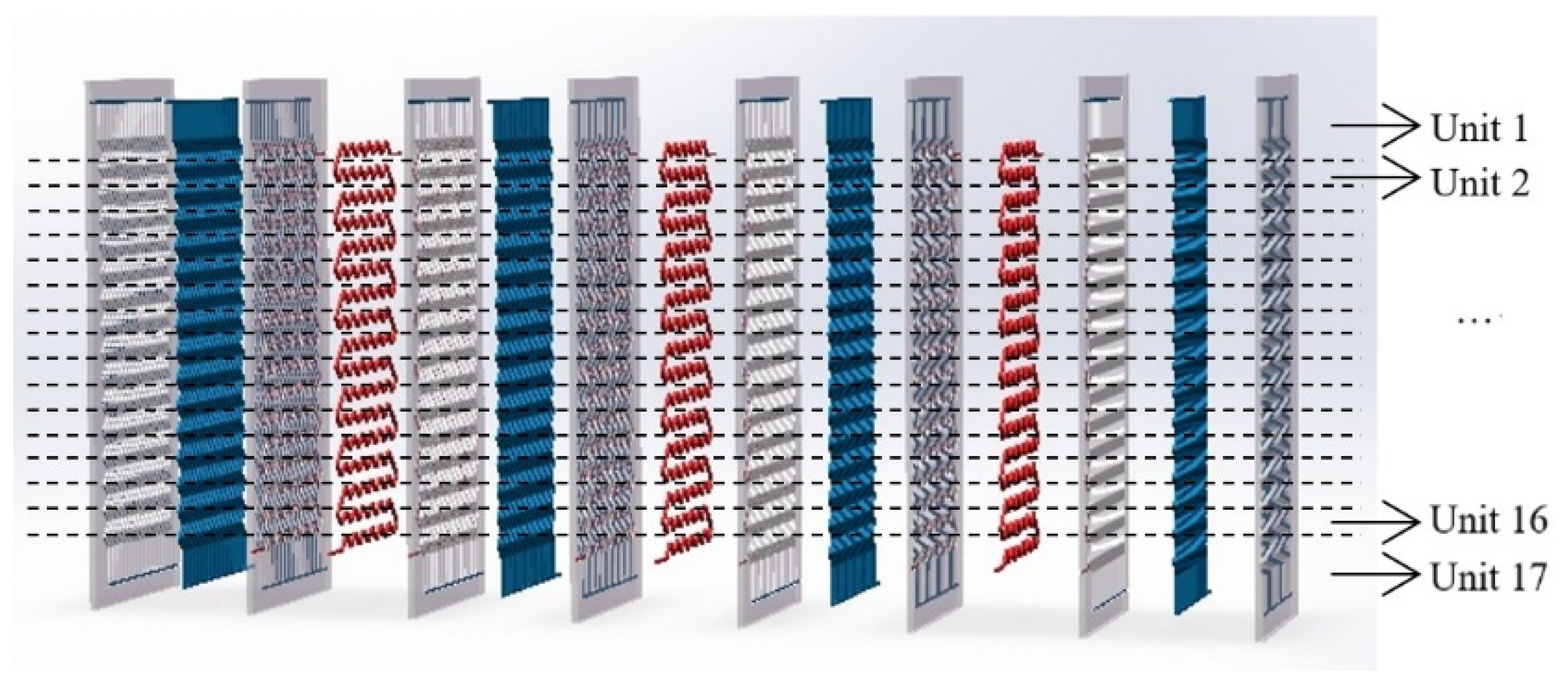
The pilot operates as a plug-flow reactor. Flow modeling is therefore based on the same hypothesis as the one used for the modeling of real continuous reactors [31,32]. The reactor is then represented by a series of perfectly stirred tank reactors (called cells). Generally, the number of cells could be defined according to the requirement of accuracy in concrete situations. To make a balance between model accuracy and calculation cost, and according to the geometry and the physical structure of the process channel, the reactor is divided into 17 computing units (see Figure 3), as there are 17 horizontal lines in each process plate. Based on previous investigations [10,18], 17 can be considered an adequate number of units for a detailed model here. Each unit contains 15 cells (see Figure 4): 3 process cells, 4 utility cells, and 8 plate wall cells. Therefore, the HEX reactor considered in this paper was divided into 255 cells in total. The far-right plate wall, as well as the far-left one, was covered by low heat transfer materials, so they are called adiabatic plates, i.e., there is no heat exchange between the reactor and environment. Thus, each process cell is a mini-reactor. It is obvious that convective heat exchange (see bi-directional arrows in Figure 4) mainly takes place between neighboring cells in the horizontal direction inside one computing unit. The flows of fluids are the connections between neighboring units.
Such description makes it very easy to represent all possible flow configurations of the reactor (co-current, counter-current). In fact, it implies that the behavior of a cell only depends on the inlet streams and phenomena taking place inside: reaction, heat transfer, etc. Since the inlets of a given cell are generally the outlets of the preceding one, any configuration of flows may be represented by correct discretization. It can also be noticed that it is easy to generalize the model to any HEX reactor by applying the number of plates and the number of cells in the plate to the actual configuration of the reactor.
The modeling of a cell is based on the expression of mass and energy balance and constraint equations. The constraint equations aim to consider the geometric characteristics of the reactor and the physical properties of the medium mentioned. The balances are used to describe the relations of the characteristic values: temperature, mass composition, etc. according to the following formula:
Given the specific geometry of the reactor, three main parts are distinguished. The first one is the process plate, where complex hydrodynamics coupled with reactions and heat transfers are found. The second one is the utility plate, where hydrodynamic and heat transfers are involved. The third one is the plate wall, which is only concerned with the heat transfer aspect.
3.2. Modeling of the Process Plate
It was considered that the process plate is sandwiched between two plate walls (right and left). Moreover, the cells representing the process plate (see Figure 5) are filled with a perfectly stirred homogeneous medium which has the following characteristics:
- Homogeneity of characteristic values (temperature, flow rate, composition, etc.).
- Homogeneity of physical properties (density, viscosity, etc.).
- Homogeneity of chemical phenomena (mixing, reaction, etc.).
- Invariable volume linked to the mixture of fluids (reactants).
The state and evolutions of the homogeneous medium circulation inside a given cell k are then described by the following balance and constraint equations:
Global mass balance (mol·s−1):
where (mol) denotes molar hold-up in process plate cell k; (mol·s−1) represents molar flow rate in process plate cell k; (mol·m−3·s−1) is production rate of the reactions; and (m3) is volume of process plate cell k.
Mass balance of component i (mol·s−1):
where represents molar fraction of component i in process plate cell k.
Process energy balance (W):
where (kg·m−3) and (J·kg−1·K−1) are density and specific heat of material in process plate cell k, respectively; (m3·s−1) is volume flow rate in process plate cell k; (K) is temperature in process plate cell k; (W·m−3) denotes heat generated by the reactions in process plate cell k; (W·m−2·K−1) and (m2) represent heat transfer coefficient and area between process plate and plate wall for cell k, respectively; and (K) and (K) are temperatures of left and right plate wall cells of the targeting cell k.
Volume constraint (m3):
where (m3) denotes maximum volume of cell k.
Due to the fact that the process plates are channels embedded in plate walls in reality, for one process plate cell, which is assumed to be a cuboid, the surface connected between process cell and plate wall cell is the four-lateral area of that cuboid. Therefore, the heat transfer area between one process cell and one plate wall cell () actually equals half of the four-lateral area. According to the principle of cell partition, each plate has 17 cells. As the targeting HEX reactor has three process plates, the total number of process cells is 51.
Thus, heat transfer area between process plate and plate wall for cell k is (m2):
where is four-sided lateral area of process channel and is computed as follows (m2):
where , , and (m) are length, width, and depth of process channel respectively.
The volume of process cell k is (m3):
where is total fluid volume of process channel and is computed as follows (m3):
3.3. Modeling of the Utility Plate and Plate Wall
To represent the reactor structure precisely, all the different heat transfer zones must be considered. Therefore, elements involved in the heat balance described by the model are as follows:
- Utility fluid plates
- Plate walls (right and left)
- Adiabatic plates
A utility plate (see Figure 6) is sandwiched between two plate walls (right and left), and the description of heat transfer is as follows:
Energy balance on the utility fluid (W):
where (kg·m−3), (m3) and (J·kg−1·K−1) are density, volume, and specific heat of material in utility plate cell k respectively; (m3·s−1) is volume flow rate in utility plate cell k; (K) is temperature in utility plate cell k; (W·m−2·K−1) and (m2) represent heat transfer coefficient and area between utility plate and plate wall for cell k, respectively.
In the same way, utility plates are also channels embedded in plate walls. As the targeting HEX reactor has four utility plates, the total quantity of utility cells is 68.
Therefore, heat transfer area between utility plate and plate wall for cell k (m2) is calculated by:
where is the four-sided lateral area of the utility channel and is computed as follows (m2):
where , , and (m) are length, width, and depth of the process channel, respectively.
The volume of utility cell k (m3) is given by:
where is total fluid volume of the utility channel and is computed as follows (m3):
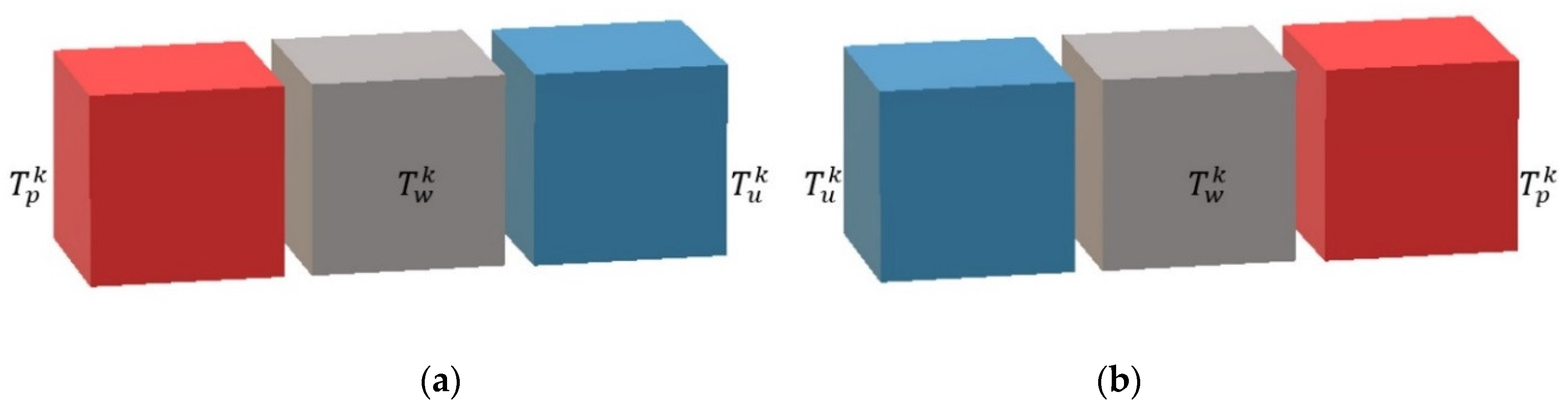
A plate wall (see Figure 7) is always sandwiched between a process plate and a utility plate, between which heat transfer is considered.
Energy balance on the plate wall (W):
where (kg·m−3), (m3) and (J·kg−1·K−1) are density, volume, and specific heat of plate wall cell k respectively; (K) is temperature of plate wall cell k.
Adiabatic plates assembled in both sides of HEX reactor are special plate walls, for which heat transfer is taking place between utility plate and environment. In this paper, it is assumed that the adiabatic plates are heat-insulated, i.e., that there is no heat transfer between adiabatic plates and the environment.
Energy balance on the adiabatic plate (W):
In fact, the plate wall cell cannot be assumed to be a cuboid, owing to the embedded channels. The exact value of the volume is obtained by its mass and density under the assumption of uniform distribution of the material. According to the dividing rules, the plant has 17 units, and each unit contains 8 plate wall cells. Thus, there are 136 plate wall cells in total.
The volume of plate wall cell k (m3) is calculated as:
where (kg) and (kg·m−3) are mass and material density of the HEX reactor.
3.4. Calculation of Heat Transfer Coefficient
As mentioned in Figure 7, the heat transfer process is divided into two parts: one is the convective heat exchange between the process channel and the plate wall, the other is between the utility channel and the plate wall. Therefore, the heat transfer ability, which is denoted by multiplying the overall heat transfer coefficient (U) and the overall heat transfer area (A), can be calculated by the convective heat transfer coefficient of the process fluid side to plate wall () and heat transfer coefficient of plate wall to utility fluid side (), which is generally defined by the following Equation (18):
where (W−1·K) is thermal resistance or fouling parameter in channels. For a clean HEX reactor, Rf is considered to be negligible.
For calculation of the overall heat transfer coefficient through pipes and channels, the Nusselt number, which represents the ratio of convective to conductive heat transfer, is an important dimensionless number. In the case of this paper, fluids inside the channels are all assumed to have the same thermal characters as water and there is no phase change. Thus, for this given HEX reactor (i.e., size, structure, and material fixed), the Reynolds number is the dominant variable in the equation of calculating . Besides, when computing the Reynolds number, the flow rate of the fluid becomes the key variable, because other parameters will have very small changes. Therefore, it can be assumed that the convective heat transfer coefficients are functions of mass flow rate and physical properties of both fluids (process and utility). For simplicity, they could be defined as linear functions in the normal operation domain, as follows:
where and are two scalar factors; and and (kg·h−1) are mass flow rates in process and utility plate, respectively.
Substitute Equations (19) and (20) into (18), then:
Experimental data concerning the HEX reactor considered in this work (see Table 2) are available, and some of them have been reported in a previous paper [9]. Using the same calculation method as in Reference [9], several values of could then be obtained. As heat transfer area and are fixed according to the geometrical properties of the HEX reactor, a genetic algorithm was introduced to search a group of optimal value for , and . The fitness function of the genetic algorithm is defined below:
where is the value of calculated from data of experiment, and and are mass flow rates of process and utility channels in the experiment.
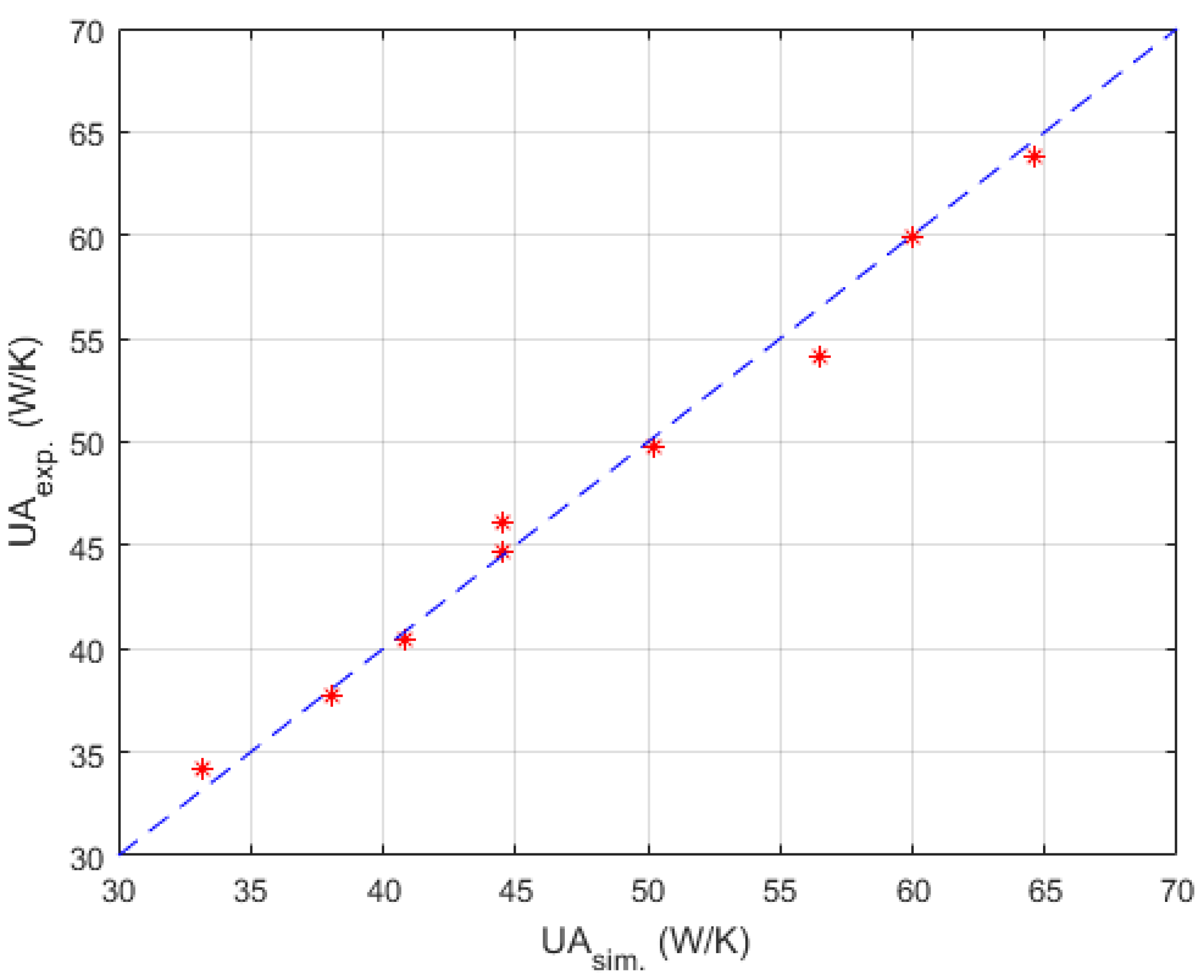
The fitness function guides the genetic algorithm to find a relatively minimal total error of Equation (21) towards experimental data. When the goal is achieved, the targeting values of , , and are found. For all the experimental data available in Table 2, we randomly reserved Experiment 5 and Experiment 8 for validation of the heat exchange simulations in Section 4. Other data of experiments in Table 2 were used here for searching relatively optimal parameters mentioned above. To prevent the algorithm dropping to a local optimal too early, the number of individuals in one generation and the number of evolutionary generations were set to 5000 and 1000 respectively. Satisfactory results were searched out, and the corresponding parity plot is shown in Figure 8.
Parameters searched by genetic algorithm are W·m−2·K−1·kg−1·h, W·m−2·K−1·kg−1·h, W−1·K. As mentioned before, is negligible. The confidence intervals depend mainly on the temperature difference between the process fluid and utility fluid. Generally, this varies from 10% to 15% of the nominal value. Thus, and were obtained in satisfactory accuracy with Equations (19) and (20).
3.5. Reaction Modeling
In order to demonstrate the advantages of the HEX reactor, experiments were carried out step by step in Reference [9].
To validate the model, the preliminary step concerned experiments with water to verify the thermal description of the reactor and the behavior of related thermal correlations. In the second step, experiments with the reaction of sodium thiosulfate oxidation by hydrogen peroxide carried out in the reactor were considered.
The reaction takes place in a homogeneous liquid phase and shows the following characteristics: irreversibility, fast kinetics, and very strong exothermicity. These features make it an ideal example for validation of the thermal and kinetic aspects of the HEX reactor and its model.
The speed of the reaction is determined by the concentration decrease of the reactants over time. As the reaction goes, the concentrations of the reactants gradually decrease.
Knowing the speed of a reaction makes it possible to estimate the rate of production for a given constituent (), the total production rate (), and the heat generated (). These estimations, which are used within the mass and energy balance of the cell, are based on the following relations:
The production rate of constituent i:
where represents stoichiometric coefficient of constituent i in reaction j.
Total production rate:
Heat generated:
where is the heat of reaction j (J·mol−1).
For the reaction of sodium thiosulfate oxidation by hydrogen peroxide, is [9]:
In this paper, the kinetic constant of reaction was assumed to be governed by an Arrhenius law, which made it possible to estimate the evolution of the constant as a function of temperature:
where () is the pre-exponential factor of the reaction j; (J·mol−1) is activation energy of reaction j; and (J·mol−1·K−1) is the perfect gas constant.
Considering the stoichiometric scheme of the reactions and Equations (23) to (26), the concentration of each reactant in a cell behaves according to the following relationships:
where and (mol·m−3) are the concentrations of and in process cell k, respectively; and is the speed of a reaction j taking place in cell k. It is expressed as a function of the concentrations of the reactants, as follows:
where (m3·mol−1·s−1) is the kinetic constant of the reaction and is given in Equation (26).
3.6. Calculating the Model in Matlab/Simulink
The formulation of the model leads to a hybrid differential and algebraic equations (DAE) system. Ordinary differential equations (ODE) (Equations (2), (3), (10), (15), (16)) contain mass and energy balances. Algebraic equations (AE) (Equations (5), (19)–(21)) consist of the reactor constraints and physical properties estimation equations. This DAE system presents a strongly nonlinear nature, mainly resulting from the modeling of the chemical reaction.
The system was modeled and simulated in Matlab/Simulink. One unit consisted of three process plate cells, four utility plate cells, and eight plate wall cells. Each cell here was called a calculating module. For process plate cells, both mass and energy balance equations were introduced in the module to take into account the evolution of the temperature and the concentrations of the components due to heat transfer and to the reaction. For utility plate and plate wall cells, only energy balance equations were considered.
Therefore, the complete pilot was represented by the connection of 17 units. For each unit, multiple inputs and outputs concerning cells in other units were elicited to connect to associate ports.
As shown in Figure 2 and Figure 3, for utility fluid, the temperature output of utility plate cell 1 in unit 1 would be connected to the temperature input of utility plate cell 1 in unit 2. For that of unit 17, it is different; the temperature output of utility plate cell 1 in unit 17 would be connected to the temperature input of utility plate cell 2 in unit 17 itself.
For process fluid, the fluid was injected at process plate cell 1 in unit 17 due to the opposite flow direction between process fluid and utility fluid. Afterward, the temperature input of process plate cell 1 in unit 16 came from the temperature output of process plate cell 1 in unit 17. The temperature output of process plate cell 1 in unit 1 was linked to process cell 2 in unit 1.
Therefore, in accordance with the general scheme of the reactor presented in Figure 2, outputs of process fluid corresponded to data of cell 3 of unit 1, and outputs of utility fluid to these of cell 4 of unit 1.
These connections maximized the heat transfer efficiency, thus, the heat generated by reactions was rapidly taken away by utility fluid. According to the manner of the connection, heat exchange mostly took place horizontally, i.e., between different kinds of cells inside a unit, due to the thin plate structure of the reactor. As a consequence, 15 cells of different plates were packed in one unit, and the heat exchange was dealt inside while the fluid flow was handled outside the unit.
4. Simulation
4.1. Initial States of the Simulations
Simulations were planned to correspond to the same situations as in experiments. In the reaction-free section, process channel and utility channel were pumped with water at different target temperatures, and flow rates of the two channels were considered as variables separately. It is natural to suppose that both the channels of the process plate and the utility plate were empty at the very beginning. The liquid was injected into the tubes only when the experiment or simulation started. Thus, for these process or utility cells, as they were considered to be connected in series, the initial condition of one cell was just the output state of the former one. The initial state of the first cell was the input state, which was the input temperature. Cells of plate wall had other initial states. Since plate wall cells are considered to form the solid reactor, their initial states were just the environment temperature, because it can be assumed that the temperature of the reactor was in equilibrium with the environment before starting the experiments. However, these initial states only affected the dynamic process. The balance states were in relation to inputs and the structure of the reactor.
4.2. Simulation Results of Heat Exchange Procedure
Operating conditions for the first part are given in Table 2. These experiments mainly focused on the inner temperature distribution of the HEX reactor under different flow rates.
Experimental data were collected from eight thermocouples. Four of them were in the first half of the process plate, which is shown in Figure 9. Two sensors were implemented at the entrance of the other two process plates, while the other two were used to detect the input temperature of the first process plate and the output temperature of the third process plate. It is obvious that all the internal sensors were located at the connecting area of two horizontal process channels. However, according to the partition rules, the output temperature of each process cell was actually the average value of that cell. Thus, after simulation, a linear interpolation between two neighboring process cells was introduced to get a more accurate calculation of sensor outputs.
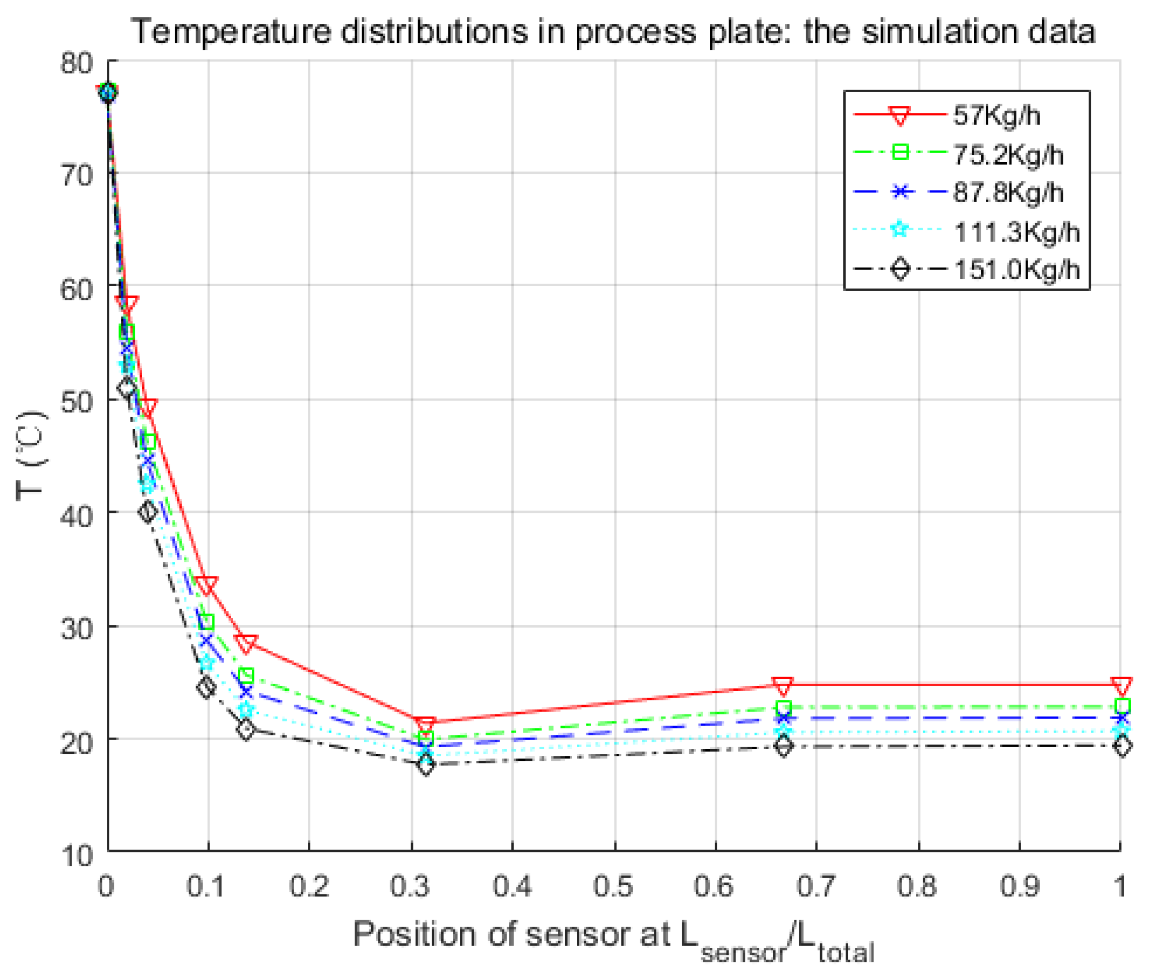
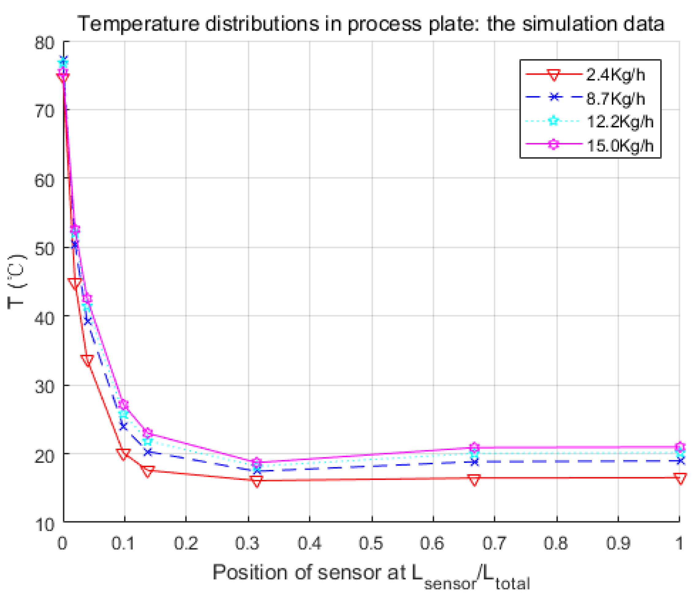
Simulations were run with the same operating conditions as the experiments. After that, data from simulations were compared with those from experiments. Figure 10 shows the simulation results of experiments 1 to 4 and 6 (corresponding to different utility flow rates), and Figure 11 presents those of experiments 7 and 9 to 11 (corresponding to different process flow rates). These two figures could be compared with Figure 12 and Figure 13, presented in Reference [9] to see the general behavior of the developed model. The Hex reactor was very efficient from heat transfer aspect, as the heat exchange process was almost completed at the first plate. When the flow rate of the process channel was fixed in Figure 10, more heat was taken away by the utility fluid as its flow rate increased. As expected, output temperature would be lower with a higher utility flow rate. This trend was opposite when the utility flow-rate was fixed in Figure 11. Output temperature would be higher if the process fluid ran more quickly. Features of these simulation results were consistent with the natural fact and the experiments reported in Reference [9]. More detailed validations were carried out using the reserved data. The computing time varied according to the performance of the computer. Generally, it took about 90 s to simulate a process of 300 s in real time on an i7-5500U platform.
There was an interesting phenomenon that nearly all the simulations had a minimal temperature at 0.33 Lsensor/Ltotal. In fact, the sensor located there was just at the entrance of the second process plate, and it was directly connected to the exit of the first process plate. As can be seen in Figure 2, we had opposite directions for the two injected fluids. For the simulation results presented in Figure 10 and Figure 11, the utility fluid had a lower temperature than the process fluid. When the process fluid started its journey in the HEX reactor, it started cooling down. When it came to the end of the first process plate, the process fluid was facing the newly injected utility fluid nearby. As, in this area, the utility fluid had the lowest temperature, it absorbed the heat through the plate wall and generated a minimal temperature for the process fluid. This was measured by the neighboring sensor at the beginning of the second process plate and presented in the figures mentioned above. Experiments presented in Reference [9] showed the same behavior.
5. Validation
To validate the accuracy and the relevance of the model and make comparisons with experiments, simulations were performed in two parts, as were the experiments. The first one concerned the heat exchange behaviors between process and utility fluid without chemical reaction. The second part introduced an exothermic chemical reaction to test the validity of the complete model. As data of Experiment 5 and Experiment 8 in Table 2 were not involved in parameter searching, simulations of these two experiments were used for the validation of the heat exchange part.
5.1. Validation of Heat Exchange Procedure
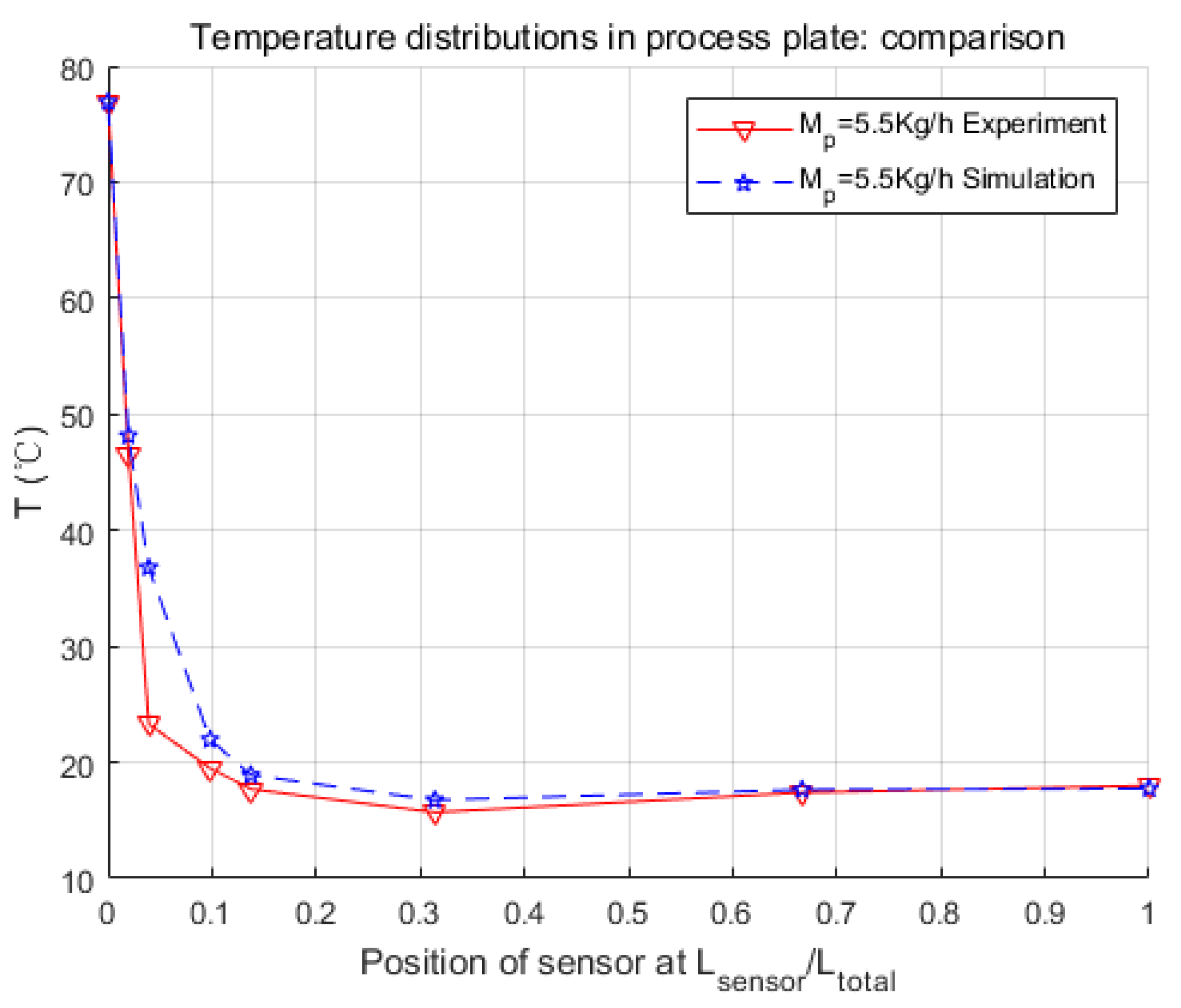
Simulations of Experiment 5 and Experiment 8 are compared with experimental data here in Figure 12 and Figure 13. Because these two groups of data were not used before in the parameter searching section, they could be used to verify if the searched parameters worked well or not.
According to Figure 12 and Figure 13, not only did temperatures obtained in simulations and experiments vary in the same manners, but their inner distributions were also close. Errors of the simulation results of the third sensor were relatively big. However, all other spots worked very well, in that they were quite close to the experimental values. Furthermore, output temperatures were identical, even though there was a little difference in the first process plate.
Based on these comparisons, the performance of the model developed in this paper in the calculation of heat exchange was acceptable. Results were highly consistent with the experiments.
5.2. Simulation Results of Heat Exchange with Reaction
In this part, concentrations of sodium thiosulfate Na2S2O3 and hydrogen peroxide H2O2 were both set to 9% in mass. Generally, it takes approximately 100 s for the reactor to reach a balance state for the heat exchange procedure without reaction. Then reactants were introduced at time t = 150 s, and the reaction began. Five simulations were launched in this part to compare with the experiments presented in Reference [9]. Table 3 gives the details of operating conditions, output temperatures, and conversion rates, which were counted in different ways.
As the concentrations were both set to 9% in mass, hydrogen peroxide H2O2 was in excess during the reaction. Therefore, the conversion rate in the simulation was calculated regarding the concentration loss of thiosulfate Na2S2O3. By contrast, in the experiments, two methods were used to calculate the conversion rates, which were based for the first on the thermal balance in the reactor, and for the second, on the use of thermal balance in a Dewar vessel after the output of the reactor (see Reference [9]).
Data in Table 3 show the interesting fact that the temperature gap between the outlets of process channel and utility channel grew smaller as the conversion rate rose. It is true that, when the conversion rate was low, the reaction took place all along the reactor till the last minute. That means materials in process channel kept generating heat, and some could not be taken away immediately in the end. Thus, the temperature gap was relatively large. While there was a higher conversion rate, the reaction mostly took place in the first plate, which left enough time for heat exchanging. Thus, the temperature gap was smaller in the end.
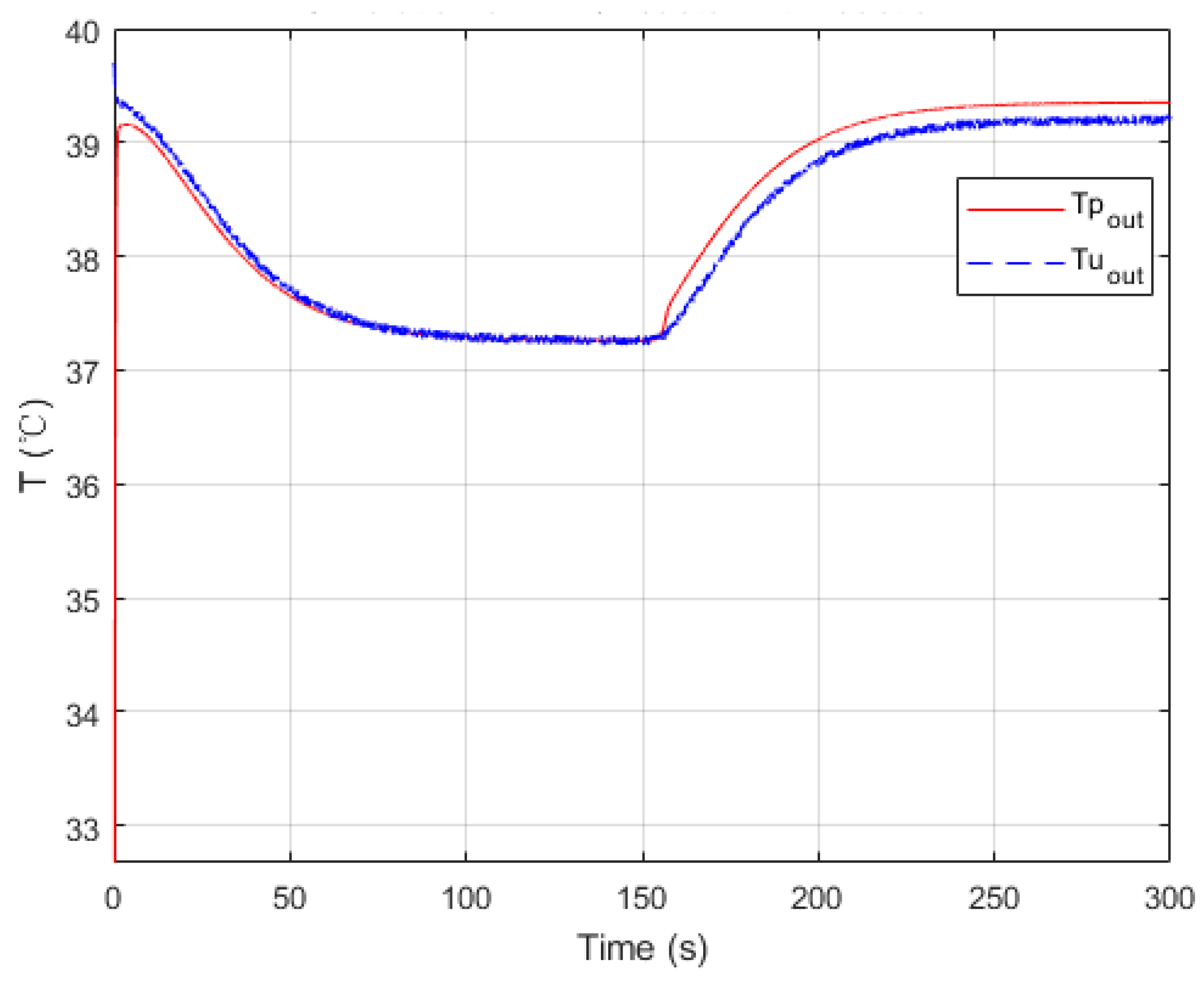
Figure 14 shows the dynamic procedure of the simulation with reaction. The steady state was reached at about 100 s. During this period, the process channel was fed with water at the same temperature as the reactants. The time it took to reach a steady state differed in the function of the operating conditions for the different experiments. Conservatively, reactants were introduced at time t = 150 s. After a residence time around 7 s, the output temperature started to change. A new steady state was reached after about 100 s. Simulations of other experiments with reaction had similar trends.
It could be noticed that the kinetic parameters of the reaction are those given by [6] and have not been fitted to the experimental data. These parameters could be renewed if there is a more accurate research about this reaction. Parameters of other reactions could also be used here to investigate the performance of the targeting HEX reactor under these reactions. For the conversion rate, experimental data calculated from the thermal balance method have errors because concentrations of products are difficult to detect precisely in mixtures. This model presents an ideal way to simulate and calculate it.
Overall, from the comparisons between experiments and simulations, it could be deduced that the model proposed in this paper is generally valid to the HEX reactor for both the heat exchange and reaction parts.
6. Conclusions
In this paper, the modeling process of an intensified HEX reactor is presented in detail, which is different from previous studies in the introducing of the chemical reaction, the modeling platform, and the combination of the physical structure and thermal features of the model. At first, the physical structure was studied, and the continuous process was discretized into cells. Consequently, the representative equations of each cell were given under the consideration of heat exchange, fluid movements, and chemical reaction. These differential equations were introduced in the general simulation platform, Matlab/Simulink. After that, three parameters concerning the heat transfer coefficient were searched by genetic algorithm, and a non-linear model of 255 basic calculating modules was developed. Finally, several simulations were launched in different working conditions to make comparisons with the experimental data.
Simulation results were quite consistent with the experiments. For the heat exchange part, this model had very accurate inner temperature distributions toward the HEX reactor. For the reaction part, this model also performed well, in that it generated good dynamic curves, as the physical one did. Furthermore, conversion rate, which is a crucial parameter to a chemical reactor, could be easily and precisely computed from the concentration loss of reactants in the model. Thus, it could be concluded that the nominal model obtained in this paper is accurate and equivalent to the real HEX reactor. One thing should be mentioned is that the modeling methodology implemented in this paper is not restricted, and could also be used for other reactions and other sizes of HEX reactors by replacing parameters to specific reactions or reactor size. The cell number could also be optimized to meet the requirements of accuracy, calculation consumption, or consistency to the physical reactor.
The purpose of modeling the HEX reactor is for further control use. With the model developed in this paper, internal states, as well as conversion rates, were easily achieved while simulating. Algorithms like model-based observers could be designed and validated conveniently on this model. These algorithms can then be used for developing approaches like fault detection, isolation, identification, and fault-tolerant control, which could be implemented on real plants to improve the performance of HEX reactors on safety, efficiency, and productivity.
Author Contributions
M.H. designed the framework that combines heat-exchange modeling, reaction modeling under the supervision of Z.L., B.D. and M.C.; M.C. collected the experimental data and reviewed the reaction mechanism; M.H. and X.H. did the simulations and validations; Z.L., M.C. and B.D. conducted the discussion and analysis of simulation results; M.H. and X.H. wrote the article, while everyone contributed in reviewing and enriching the content.
Funding
This research was funded by the Department of Science and Technology of Guizhou, grand numbers [2015]4014, [2015]11, [2016]2302, [2019]2154 and the Department of Education of Guizhou, grand number ZDXK [2015]8.
Acknowledgments
The authors gratefully acknowledge financial support provided by China Scholarship Council (CSC). The authors also acknowledge Elsevier for the copyright permission of reprinting materials in [9].
Conflicts of Interest
The authors declare no conflict of interest.
Nomenclature
| Roman Letters | |
| area (m2) | |
| concentration of constituent (mol·m−3) | |
| specific heat (J·kg−1·K−1) | |
| activation energy of reaction (J·mol−1) | |
| molar flow-rate (mol·s−1) | |
| volume flow-rate (m3·s−1) | |
| heat transfer coefficient (W·m−2·K−1) | |
| heat of reaction (J·mol−1) | |
| experiment i | |
| fitness function of the genetic algorithm | |
| kinetic constant of the reaction () | |
| length (m) | |
| mass (kg) | |
| mass flow-rate (kg·h−1) | |
| production rate of the reactions (mol·m−3·s−1) | |
| speed of reaction (mol·m−3·s−1) | |
| perfect gas constant (J·mol−1·K−1) | |
| Rf | thermal resistance or fouling parameter in channels (W−1·K) |
| temperature (K) | |
| molar hold-up (mol) | |
| overall heat transfer coefficient (W·m−2·K−1) | |
| volume (m3) | |
| molar fraction of component | |
| Greek Letters | |
| scale factor in calculating | |
| scale factor in calculating | |
| density (kg·m−3) | |
| stoichiometric coefficient of a constituent in a reaction | |
| Subscripts | |
| constituent i | |
| reaction j | |
| left | |
| process plate | |
| reactor | |
| right | |
| utility plate | |
| plate wall | |
| Superscript | |
| cell k |
References
- Green, A.; Johnson, B.; Arwyn, J. Process intensification magnifies profits. Chem. Eng. 1999, 106, 66–73. [Google Scholar]
- Hendershot, D.C. Process minimization: Making plants safer. Chem. Eng. Prog. 2000, 96, 35–40. [Google Scholar]
- Etchells, J.C. Process intensification: Safety pros and cons. Process. Saf. Environ. Prot. 2005, 83, 85–89. [Google Scholar] [CrossRef]
- Stitt, E.H. Alternative multiphase reactors for fine chemicals: A world beyond stirred tanks? Chem. Eng. J. 2002, 90, 47–60. [Google Scholar] [CrossRef]
- Phillips, C.H.; Lauschke, G.; Peerhossaini, H. Intensification of batch chemical processes by using integrated chemical reactor-heat exchangers. Appl. Therm. Eng. 1997, 17, 809–824. [Google Scholar] [CrossRef]
- Anxionnaz, Z.; Cabassud, M.; Gourdon, C.; Tochon, P. Heat exchanger/reactors (HEX reactors): Concepts, technologies: State-of-the-art. Chem. Eng. Process. Process. Intensif. 2008, 47, 2029–2050. [Google Scholar] [CrossRef] [Green Version]
- Benaissa, W.; Elgue, S.; Gabas, N.; Cabassud, M.; Carson, D.; Demissy, M. Dynamic behaviour of a continuous heat exchanger/reactor after flow failure. Int. J. Chem. React. Eng. 2010, 8. [Google Scholar] [CrossRef]
- Bahroun, S.; Li, S.; Jallut, C.; Valentin, C.; Panthou, F. De Control and optimization of a three-phase catalytic slurry intensified continuous chemical reactor. J. Process. Control. 2010, 20, 664–675. [Google Scholar] [CrossRef]
- Théron, F.; Anxionnaz-Minvielle, Z.; Cabassud, M.; Gourdon, C.; Tochon, P. Characterization of the performances of an innovative heat-exchanger/reactor. Chem. Eng. Process. Process. Intensif. 2014, 82, 30–41. [Google Scholar] [CrossRef] [Green Version]
- Anxionnaz-Minvielle, Z.; Cabassud, M.; Gourdon, C.; Tochon, P. Influence of the meandering channel geometry on the thermo-hydraulic performances of an intensified heat exchanger/reactor. Chem. Eng. Process. Process. Intensif. 2013, 73, 67–80. [Google Scholar] [CrossRef] [Green Version]
- Škrjanc, I.; Matko, D. Predictive functional control based on fuzzy model for heat-exchanger pilot plant. IEEE Trans. Fuzzy Syst. 2000, 8, 705–712. [Google Scholar] [CrossRef]
- Vasičkaninová, A.; Bakošová, M.; Mészáros, A.; Klemeš, J.J. Neural network predictive control of a heat exchanger. Appl. Therm. Eng. 2011, 31, 2094–2100. [Google Scholar] [CrossRef] [Green Version]
- Oravec, J.; Bakosova, M.; Meszaros, A. Robust Model Predictive Control of Heat Exchangers in Series. Chem. Eng. Trans. 2016, 52, 253–258. [Google Scholar]
- Escobar, R.F.; Astorga-Zaragoza, C.M.; Tllez-Anguiano, A.C.; Jurez-Romero, D.; Hernndez, J.A.; Guerrero-Ramrez, G.V. Sensor fault detection and isolation via high-gain observers: Application to a double-pipe heat exchanger. ISA Trans. 2011, 50, 480–486. [Google Scholar] [CrossRef]
- Persin, S.; Tovornik, B. Real-time implementation of fault diagnosis to a heat exchanger. Control. Eng. Pract. 2005, 13, 1061–1069. [Google Scholar] [CrossRef]
- Jonsson, G.R.; Lalot, S.; Palsson, O.P.; Desmet, B. Use of extended Kalman filtering in detecting fouling in heat exchangers. Int. J. Heat Mass Transf. 2007, 50, 2643–2655. [Google Scholar] [CrossRef]
- Astorga-Zaragoza, C.M.; Zavala-Río, A.; Alvarado, V.M.; Méndez, R.M.; Reyes-Reyes, J. Performance monitoring of heat exchangers via adaptive observers. Meas. J. Int. Meas. Confed. 2007, 40, 392–405. [Google Scholar] [CrossRef]
- Zhang, M.; Li, Z.; Cabassud, M.; Dahhou, B. An integrated FDD approach for an intensified HEX/Reactor. J. Control. Sci. Eng. 2018, 2018. [Google Scholar] [CrossRef]
- Zhang, M.; Dahhou, B.; Cabassud, M.; Li, Z.T. Faults isolation and identification of Heat-exchanger/Reactor with parameter uncertainties. In Proceedings of the 26th International Workshop on Principles of Diagnosis, Paris, France, 31 August 2015. [Google Scholar]
- Li, Z.; Dahhou, B.; Zhang, M.; Cabassud, M. Actuator gain fault diagnosis for heat-exchanger/reactor. 2015 Chinese Autom. Congr. (CAC) 2015, 940–945. [Google Scholar]
- Sotomayor, O.A.Z.; Odloak, D. Observer-based fault diagnosis in chemical plants. Chem. Eng. J. 2005, 112, 93–108. [Google Scholar] [CrossRef]
- Ball, R.; Gray, B.F. Thermal instability and runaway criteria: The dangers of disregarding dynamics. Process. Saf. Environ. Prot. 2013, 91, 221–226. [Google Scholar] [CrossRef] [Green Version]
- Zavala-Río, A.; Santiesteban-Cos, R. Reliable compartmental models for double-pipe heat exchangers: An analytical study. Appl. Math. Model. 2007, 31, 1739–1752. [Google Scholar] [CrossRef] [Green Version]
- Mathisen, K.W.; Morari, M.; Skogestad, S. Dynamic models for heat exchangers and heat exchanger networks. Comput. Chem. Eng. 1994, 18, S459–S463. [Google Scholar] [CrossRef]
- Varbanov, P.S.; Klemeš, J.J.; Friedler, F. Cell-based dynamic heat exchanger models—Direct determination of the cell number and size. Comput. Chem. Eng. 2011, 35, 943–948. [Google Scholar] [CrossRef]
- Bracco, S.; Faccioli, I.; Troilo, M. A numerical discretization method for the dynamic simulation of a double-pipe heat exchanger. Int. J. Energy 2007, 1, 47–58. [Google Scholar]
- Weyer, E.; Szederkényi, G.; Hangos, K. Grey box fault detection of heat exchangers. Control. Eng. Pract. 2000, 8, 121–131. [Google Scholar] [CrossRef]
- Anxionnaz, Z.; Theron, F.; Tochon, P.; Couturier, R.; Bucci, P.; Vidotto, F.; Gourdon, C.; Cabassud, M.; Lomel, S.; Bergin, G.; et al. RAPIC project: Toward competitive heat-exchanger/reactors. In Proceedings of the The 3rd European Process Intensification Conference (EPIC), Manchester, UK, 20 June 2011. [Google Scholar]
- Tochon, P.; Couturier, R.; Anxionnaz, Z.; Lomel, S.; Runser, H.; Picqrd, F.; Colin, A.; Gourdon, C.; Cabassud, M.; Peerhossqini, H.; et al. Toward a competitive process intensification: A new generation of heat exchanger-reactors. Oil Gas. Sci. Technol. 2010, 65, 785–792. [Google Scholar] [CrossRef]
- Tochon, P.; Couturier, R.; Vidotto, F. Method for producing a heat exchanger system, preferably of the exchanger/reactor type. U.S. Patent 8468697B2, 2013. [Google Scholar]
- Westerterp, K.R.; Van Swaaij, W.P.M.; Beenackers, A.A.C.M.; Kramers, H. Chemical reactor design and operation, 2nd ed.; Wiley: Hoboken, NJ, USA, 1987. [Google Scholar]
- Nauman, E.B. Chemical Reactor Design, Optimization, and Scaleup; John Wiley: Hoboken, NJ, USA, 2008. [Google Scholar]
Figure 1.
Details of the heat exchanger/reactor: (a) Process channel; (b) utility channel; (c) the heat exchanger/reactor after assembly [9].
Figure 1.
Details of the heat exchanger/reactor: (a) Process channel; (b) utility channel; (c) the heat exchanger/reactor after assembly [9].
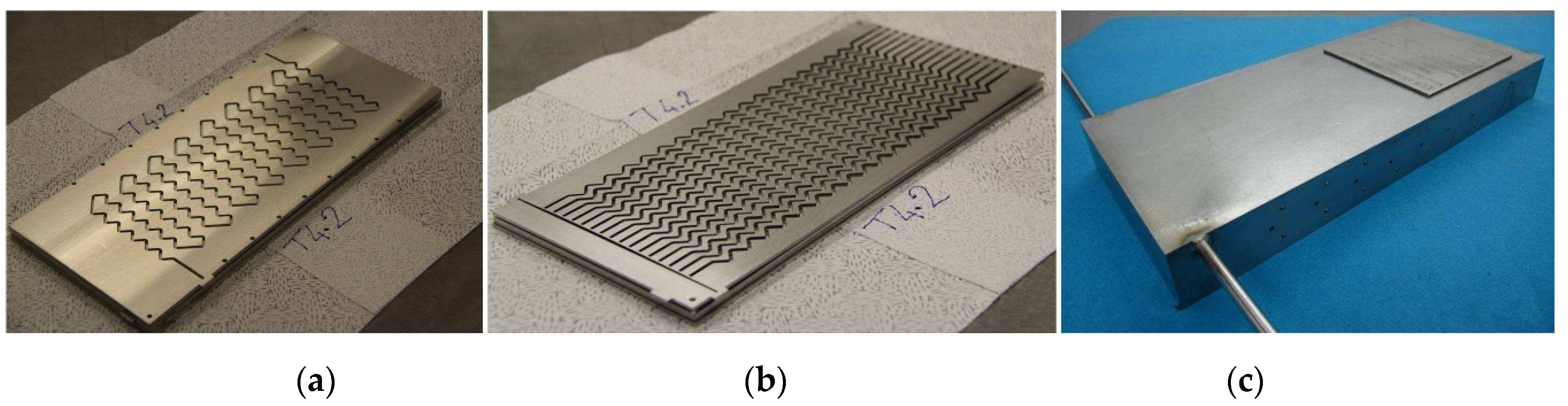
Figure 2.
Block modeling description, showing (a) utility plate, (b) process plate, and (c) plate wall.
Figure 2.
Block modeling description, showing (a) utility plate, (b) process plate, and (c) plate wall.
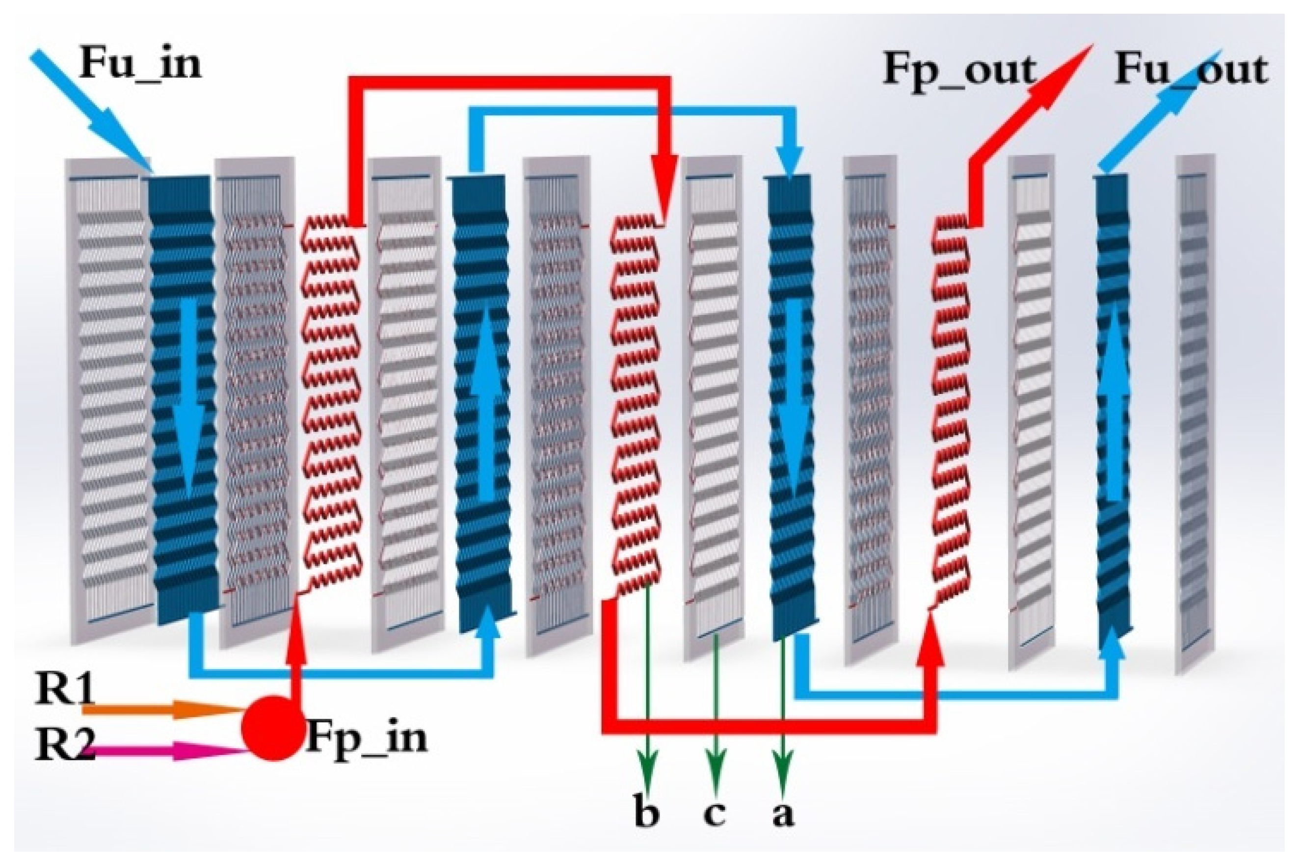
Figure 3.
Description of units dividing.

Figure 4.
Internal description of one computing unit and convective heat exchange.
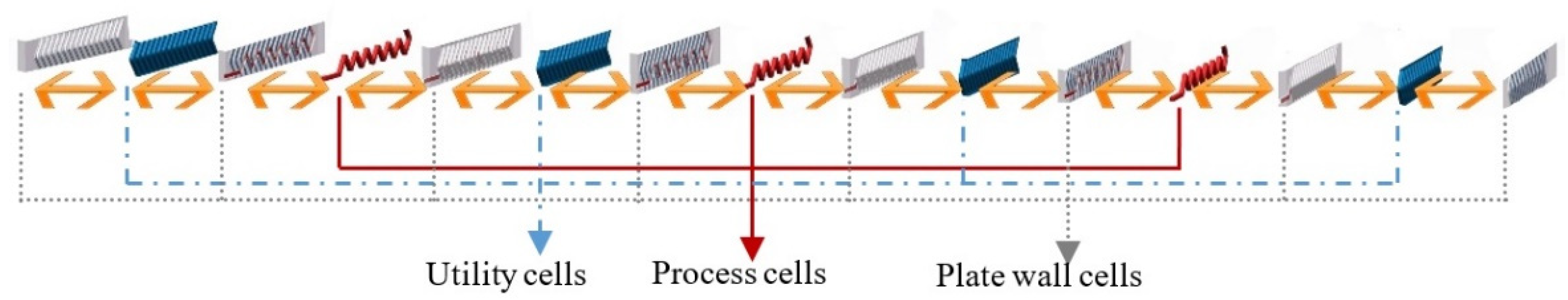
Figure 5.
Representation of a cell k of process plate.
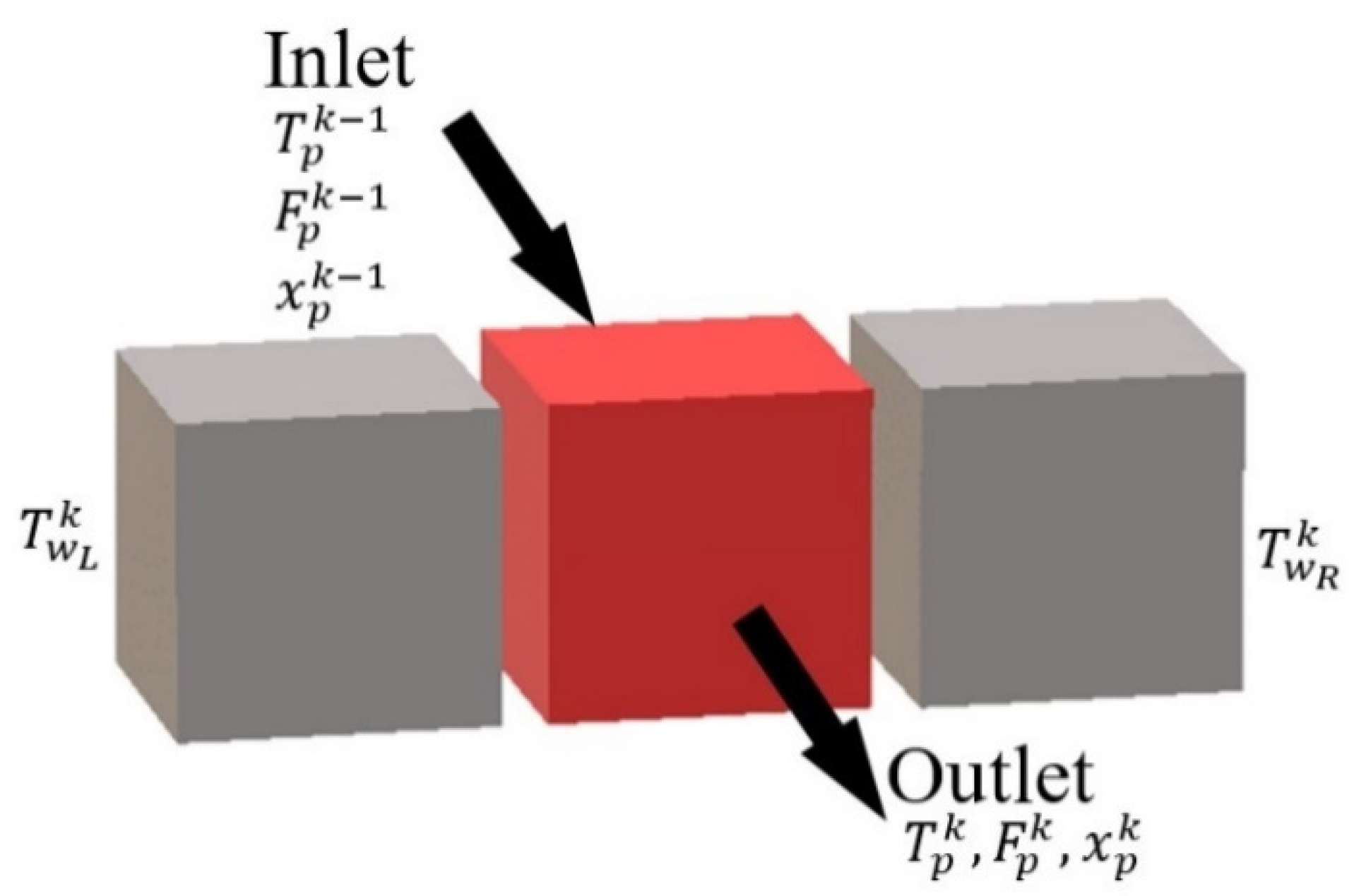
Figure 6.
Representation of a cell k of utility plate.
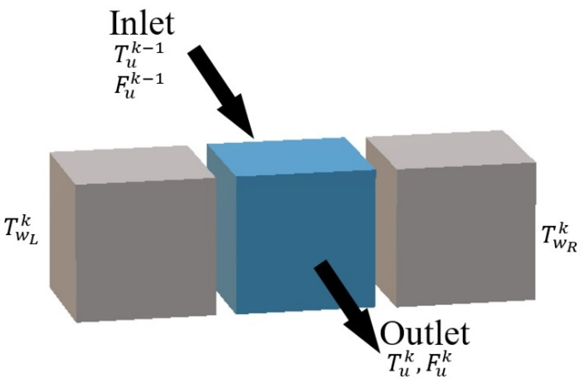
Figure 7.
(a) Representation of a cell k of plate wall with process plate in the left and utility plate in the right; (b) Representation of a cell k of plate wall with process plate in the right and utility plate in the left.
Figure 7.
(a) Representation of a cell k of plate wall with process plate in the left and utility plate in the right; (b) Representation of a cell k of plate wall with process plate in the right and utility plate in the left.

Figure 8.
Parity plot of (the overall heat transfer coefficient () and the overall heat transfer area ()) calculated from experimental data against those given by Equation (21) using the searched values of , , and .
Figure 8.
Parity plot of (the overall heat transfer coefficient () and the overall heat transfer area ()) calculated from experimental data against those given by Equation (21) using the searched values of , , and .

Figure 9.
Localization of five thermocouples in the first process plate [9].
Figure 9.
Localization of five thermocouples in the first process plate [9].
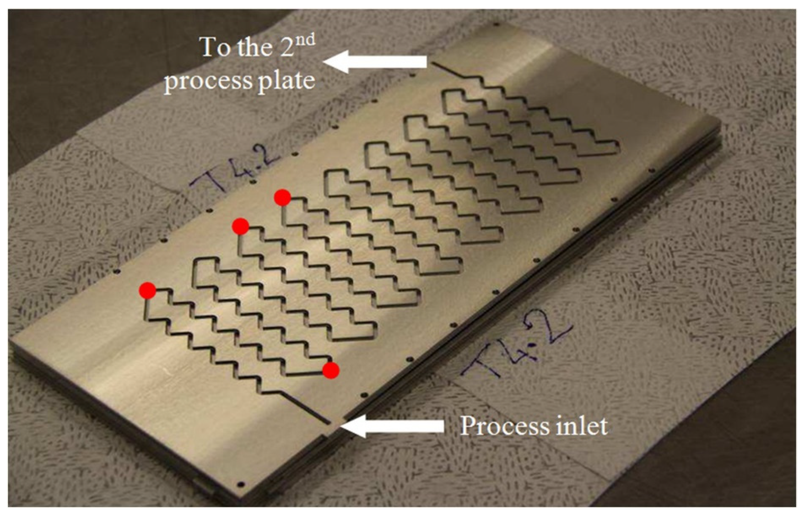
Figure 10.
Simulation results of the process fluid temperature along the process channel for different utility flow rates, with = 10 kg·h−1 and = 77 °C.
Figure 10.
Simulation results of the process fluid temperature along the process channel for different utility flow rates, with = 10 kg·h−1 and = 77 °C.

Figure 11.
Simulation results of the process fluid temperature along the channel for different process flow rates, with = 152 kg·h−1 and = 15.6 °C.
Figure 11.
Simulation results of the process fluid temperature along the channel for different process flow rates, with = 152 kg·h−1 and = 15.6 °C.

Figure 12.
Comparison of inner temperature distribution of Experiment 5 with = 10 kg·h−1 and = 77 °C
Figure 12.
Comparison of inner temperature distribution of Experiment 5 with = 10 kg·h−1 and = 77 °C
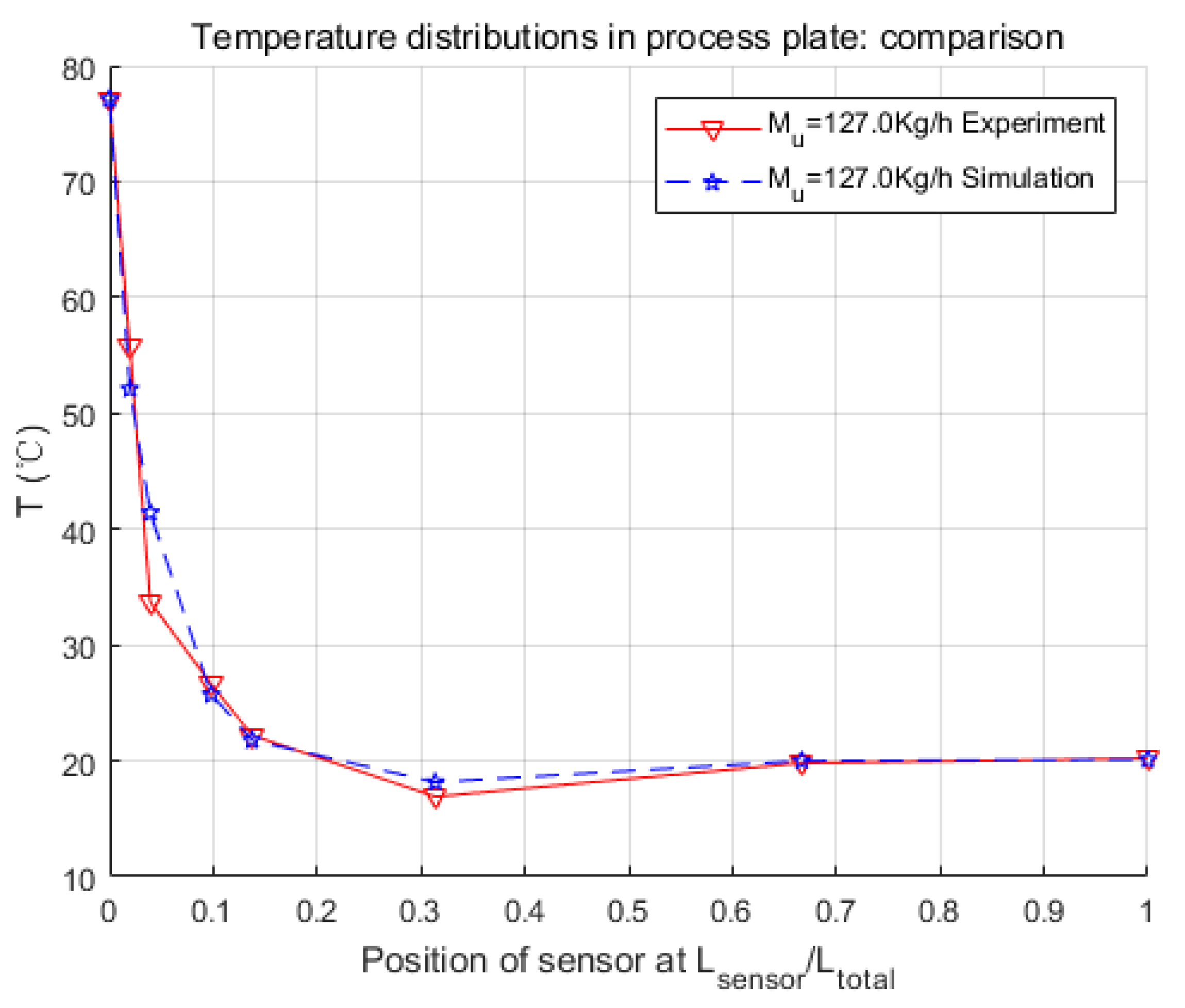
Figure 13.
Comparison of inner temperature distribution of Experiment 8 with = 152 kg·h−1 and = 15.6 °C.
Figure 13.
Comparison of inner temperature distribution of Experiment 8 with = 152 kg·h−1 and = 15.6 °C.

Figure 14.
Simulated temperature profiles for experiment 1 (reaction was introduced at 150 s).


Table 1.
Geometrical properties of the heat-exchanger/reactor [9].
Table 1.
Geometrical properties of the heat-exchanger/reactor [9].
| Process Stream | Utility Stream | |
|---|---|---|
| Number of parallel channels | 1 | 16 |
| Number of plates for each stream | 3 | 4 |
| Individual channel width Lwidth (mm) | 2.0 | 2.0 |
| Individual channel depth Ldepth (mm) | 2.0 | 2.0 |
| Total channel length, Ltotal (mm) | 6.7 × 10³ | 2.8525 × 10⁴ |
| Hydraulic diameter, Dh (mm) | 2.0 | 2.0 |
| Total fluid volume (mm3) | 2.68 × 10⁴ | 1.141 × 10⁵ |
| Metal thickness between streams (mm) | 2.0 | 2.0 |
Table 2.
Experimental conditions for simulating the heat exchange experiments [9].
Table 2.
Experimental conditions for simulating the heat exchange experiments [9].
| Experiment No. | Utility Stream | Process Stream | ||
|---|---|---|---|---|
| (kg·h−1) | (°C) | (kg·h−1) | (°C) | |
| 1 | 57.0 | ≈15.6 | ≈10.0 | ≈77.0 |
| 2 | 75.2 | |||
| 3 | 87.8 | |||
| 4 | 111.3 | |||
| 5 | 127.0 | |||
| 6 | 151.0 | |||
| 7 | ≈152.0 | ≈15.6 | 2.4 | ≈77.0 |
| 8 | 5.5 | |||
| 9 | 8.7 | |||
| 10 | 12.2 | |||
| 11 | 15.0 | |||
Table 3.
Comparisons of experiment and simulation data with reaction.
| Data Source | Operating Condition | Output Temperature | Conversion Rate (%) | |||||||
|---|---|---|---|---|---|---|---|---|---|---|
| (L·h−1) (Na2S2O3) | (L·h−1) (H2O2) | (°C) | (kg·h−1) | (°C) | (°C) | (°C) | Reactor | Dewar | C1 (Na2S2O3) | |
| Experiment 1 | 9.3 | 4.7 | 17.6 | 113.0 | 39.7 | 43.9 | 39.9 | 60 | 59 | – |
| Simulation 1 | 39.4 | 39.2 | – | – | 67 | |||||
| Experiment 2 | 3.3 | 1.7 | 19.3 | 113.5 | 39.7 | 41.4 | 40.4 | 82 | 94 | – |
| Simulation 2 | 39.9 | 39.8 | – | – | 90 | |||||
| Experiment 3 | 4.7 | 2.3 | 20.0 | 113.0 | 39.7 | 43.4 | 41.1 | 88 | 91 | – |
| Simulation 3 | 39.9 | 39.8 | – | – | 83 | |||||
| Experiment 4 | 4.7 | 2.3 | 20.7 | 112.0 | 49.6 | 51.0 | 50.7 | 93 | 100 | – |
| Simulation 4 | 49.4 | 49.4 | – | – | 94 | |||||
| Experiment 5 | 4.7 | 2.3 | 21.1 | 112.5 | 59.4 | 59.2 | 60.1 | 95 | 100 | – |
| Simulation 5 | 58.7 | 58.7 | – | – | 99 | |||||
1 C (Na2S2O3) denotes that conversion rates below are calculated by the concentration loss of Na2S2O3.
© 2019 by the authors. Licensee MDPI, Basel, Switzerland. This article is an open access article distributed under the terms and conditions of the Creative Commons Attribution (CC BY) license (http://creativecommons.org/licenses/by/4.0/).
Share and Cite
MDPI and ACS Style
He, M.; Li, Z.; Han, X.; Cabassud, M.; Dahhou, B. Development of a Numerical Model for a Compact Intensified Heat-Exchanger/Reactor. Processes 2019, 7, 454. https://doi.org/10.3390/pr7070454
AMA Style
He M, Li Z, Han X, Cabassud M, Dahhou B. Development of a Numerical Model for a Compact Intensified Heat-Exchanger/Reactor. Processes. 2019; 7(7):454. https://doi.org/10.3390/pr7070454
Chicago/Turabian StyleHe, Menglin, Zetao Li, Xue Han, Michel Cabassud, and Boutaib Dahhou. 2019. "Development of a Numerical Model for a Compact Intensified Heat-Exchanger/Reactor" Processes 7, no. 7: 454. https://doi.org/10.3390/pr7070454
Note that from the first issue of 2016, this journal uses article numbers instead of page numbers. See further details here.