1. Introduction
Population balance models (PBMs) show a significant role in different areas of science and engineering. These models have numerous applications in high-energy physics, geophysics, biophysics, meteorology, pharmacy, food science, chromatography, chemical engineering, civil engineering, and environmental engineering. These models are used in the process of cell dynamics, polymerization, cloud formation, and crystallization. In biophysics, these models are concerned with population of various kinds of cells. Population balance models are also used in the formation of ceramics mixtures and nanoparticles which have a lot of applications.
In 1964, Hulburt & Katz [
1] were first to discuss the PBMs in chemical engineering. A detailed description of these models is given in [
2]. The main components in the models are the process of nucleation, growth, aggregation, breakage, inlet, outlet, growth, and dissolution. The mathematical model of population balance equations are partial integro-differential equations (PIDEs). Analytical solutions of these PIDEs are very rare except for a few simple cases. Therefore, researchers are interested in developing numerical solutions for these equations. Numerous numerical methods are accessible in the literature to solve certain kinds of PBMs; see, for example, [
3,
4,
5,
6,
7,
8,
9,
10,
11].
The Quadrature Method of Moments (QMOM) for solving the governed models was first introduced by McGraw [
12]. The direct QMOM was proposed by Fan et al. [
4]. In addition, a new QMOM has been proposed by Gimbun [
5]. Qamar et al. [
13] introduced an alternative QMOM for solving length-based batch crystallization models telling crystals nucleation, size-dependent growth, aggregation, breakage, and dissolution of small nuclei below certain critical size. Safyan et al. [
14] followed the technique of [
13] for solving volume-based batch crystallization model nucleation, size-dependent growth, aggregation, breakage. In this article, the QMOM is used to solve volume-based batch crystallization models with fines dissolution. The fines dissolution unit improves the product quality and removes unwanted particles.
In the proposed method, orthogonal polynomials, taken from the lower-order moments, are used to find the quadrature points and weights. For confirming accuracy of the scheme, a third-order orthogonal polynomial, employing the first six moments, was chosen to estimate the quadrature points (abscissas) and equivalent quadrature weights. Hence, it was essential to solve at least a six-moment system (i.e., 0, …, 5). This type of polynomial provides a three-point Gaussian quadrature rule which usually produces precise output for polynomials of degree five or less. The expression for the preferred orthogonal polynomial can be derived analytically and the mandatory number of moments rises with order of polynomial. It is important to mention that the calculation of six moments to generate each time the third-order polynomial is compulsory. However, the technique itself is not limited to the calculation of every listed number of moments. The calculation of additional moments is conducted by adding ordinary differential equation.
This article is divided into two parts: In the first part, the mathematical model of volume-based Population Balance Equation (PBE) with fines dissolution is presented. In the second part, the proposed QMOM is derived for PBEs. Furthermore, the mathematical outcomes of QMOM are compared with the analytical outcomes that are accessible in literature.
2. Materials and Methods
Suppose
represents the number density function, then a general PBE is given by [
1,
2]:
where
. The variable
represents the time and
may be size, length, or composition. In this article, it represents the particle volume. In the above equation, each term has its specific definition. These terms are given by
where
and
Here,
represents the birth of particles of volume
resulting for amalgamation of two particles with respective volume
and
where
and
is the death of particles, describing the decrease in particle volume
by aggregation with other particles of any volume. The aggregation kernel
is the rate at which aggregation of two particles
and
produces a particle volume
.
where
and
Here,
represents the birth of new particles during the breakage process and the breakage function
is the probability density function for the formation of particle volume
from particle volume
, whereas,
is the death of particles, and
is the selection function describing the rate at which the particles are selected to break.
represents the dissolution term,
is the volume of crystallizer,
is the volumetric flow rate from the crystallizer to dissolution unit,
is the dissolution function describing dissolution of small particles below some critical size. The population balance equation can be simplified through introducing the moment function. The
moment of the population density function is mathematically written in the form:
The first and second moments
denote particle population and volume, respectively, at any instant
. Multiply
to left- and right-hand side of Equation (1) and at that moment integrate it over the volume
, so we obtain the following equation:
where
The aggregation terms
and
are mathematically defined as
whereas
and
are birth and death functions because of breakage term and are given by
Due to aggregation, the upper limit in the birth function is not infinity; therefore, we cannot apply quadrature method of moment for this integral. To apply the QMOM, we have to convert the upper limit to infinity. Here, we introduce a Heaviside step function
to solve the integral such that
when
and
otherwise. As a result, we will find the limits of integration over
from
to
. Thus, by applying it to the birth function, we obtain the following equation:
On the right side of Equation (7), we have switched the order of integration and made the replacement
Lastly, we have replaced
for
with no damage of generality and caught the necessary outcome for birth due to aggregation which is given by
After substituting all of the above terms in Equation (6), we get the system of differential equations:
In addition, with solid phase, the liquid phase yields ordinary differential equation for the solute mass in the form:
with
where
is the density of crystals and
is a volume shape factor.
is the incoming mass flux from dissolution unit to crystallizer and outgoing mass flux from crystallizer to dissolution unit, respectively, which is mathematically defined by
where
is the mass of solvent and
is the density of the solution.
is the residence time in the dissolution unit, where
represents volume of the pipe.
Here, we will consider the Gaussian quadrature method to solve the complicated integral terms appearing in Equations (8) and (9). Consequently, a closed-form system of moments is found. Further, we have accurately and efficiently solved the closed-form system with an ODE solver. The approximation of definite integral with the help of quadrature rule is an important numerical aspect. For this purpose, first we calculate the function at definite points and then use the formula of weight function which gives approximation of the definite integral. To approximate a definite integral given in Equations (8) and (9), first we find the values of the function at a set of equidistant points. After evaluating, the weight function is multiplied to approximate the integrals. In this rule, there is no limitation of choosing abscissas and weights. This rule also works for the points which are not likewise spread out. Let us assume the integral of the formula
. We can find the weights
and abscissas
by approximating the definite integral as
where provided it is exact and
is smooth function. A set of orthogonal polynomials is necessary for making certain
order orthogonal polynomial and it should contain only one polynomial of order
for
. We can define the scalar product of the two functions
and
over a weight function
by
If we find the zero scalar product of any two functions
and
, then these functions are termed as orthogonal functions. It is also noted that supplementary information will be required for obtaining abscissas and weights if the classical weight function
is not provided. For this purpose, we have used the moment:
In the above equation,
is used as a weight function
.
given in Equation (13) denotes the polynomial
of
order. To find
abscissas weights, we need
moments from
to
. For
this approximation will be exact. For simplicity and accurate approximations, we set
. As a result, six-moment system for
is calculated. To discuss the procedure, we consider ODEs (8) and (9). Using Equation (13) in Equations (8) and (9), we obtain the following equations:
where
and
Our next step is computing the quadrature points
and the quadrature weights
. The quadrature points
are obtained from the roots of orthogonal polynomials. The construction of orthogonal polynomials is described as follows:
with
Since the function
is used as a weight function
, so from Equation (12) we have
Using all of the above definitions, the orthogonal polynomials of any order can be obtained. Our first step is to find the roots of the
order polynomial. The quadrature points
are then obtained from these roots. To explain the procedure of deriving these orthogonal polynomials, we have calculated
,
.
as
First,
will be calculated, which is given by
so
Again from Equations (17) and (18) we have
and
so from Equation (20) we have
Proceeding in a similar way, we can calculate the polynomial of higher order. The third-order polynomial
is given by the following equation:
The roots of the selected polynomial will give us the abscissas
. Next, the weights
will be calculated. According to Press et al. [
15], the expression for the weight function is given by
where
N is the order of the selected polynomial. At last, the resulting system of ODEs is then solved by any standard ODE solver in MatLab.
3. Results
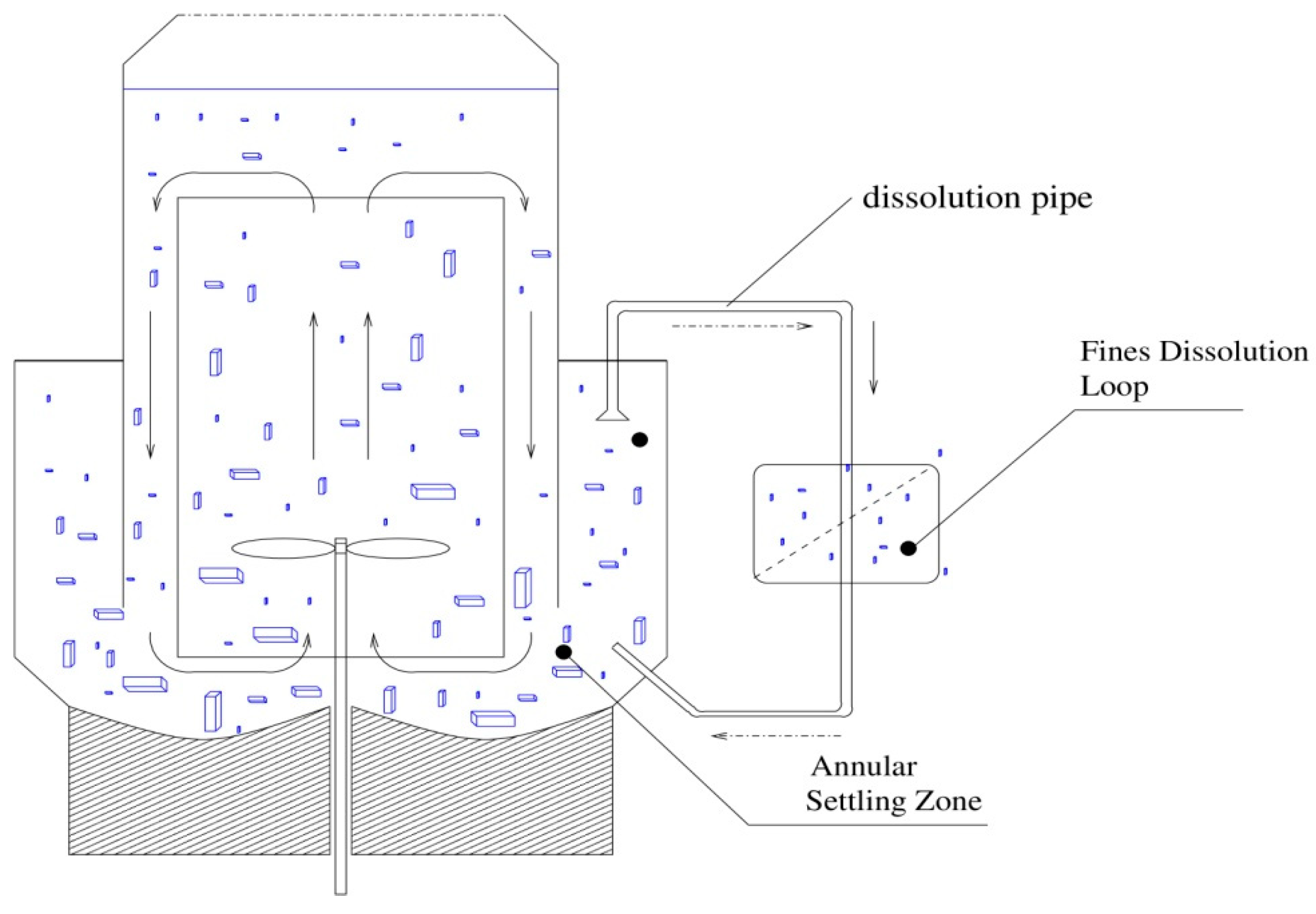
Test Problem 1: Aggregation with Fines Dissolution
Here, the proposed scheme is analyzed for aggregation with fines dissolution (see
Figure 1) problem encountered in several particulate methods (i.e., fluidized beds, formation of rain droplets, and manufacture of dry powders). The effects of further procedures, such as breakage, growth, and nucleation, are negligible. During the aggregation process, the total mass of particles
is conserved and the amount of particles
reduces during the processing time. The aggregation kernel is held to be constant and is defined as
, where
. The exponential initial particle size distribution is given by
where
and
. The dissolution term
explains the dissolution of particles below certain critical size, that is,
. The analytical solution in terms of the number density
is given by Scott [
16]:
where
and
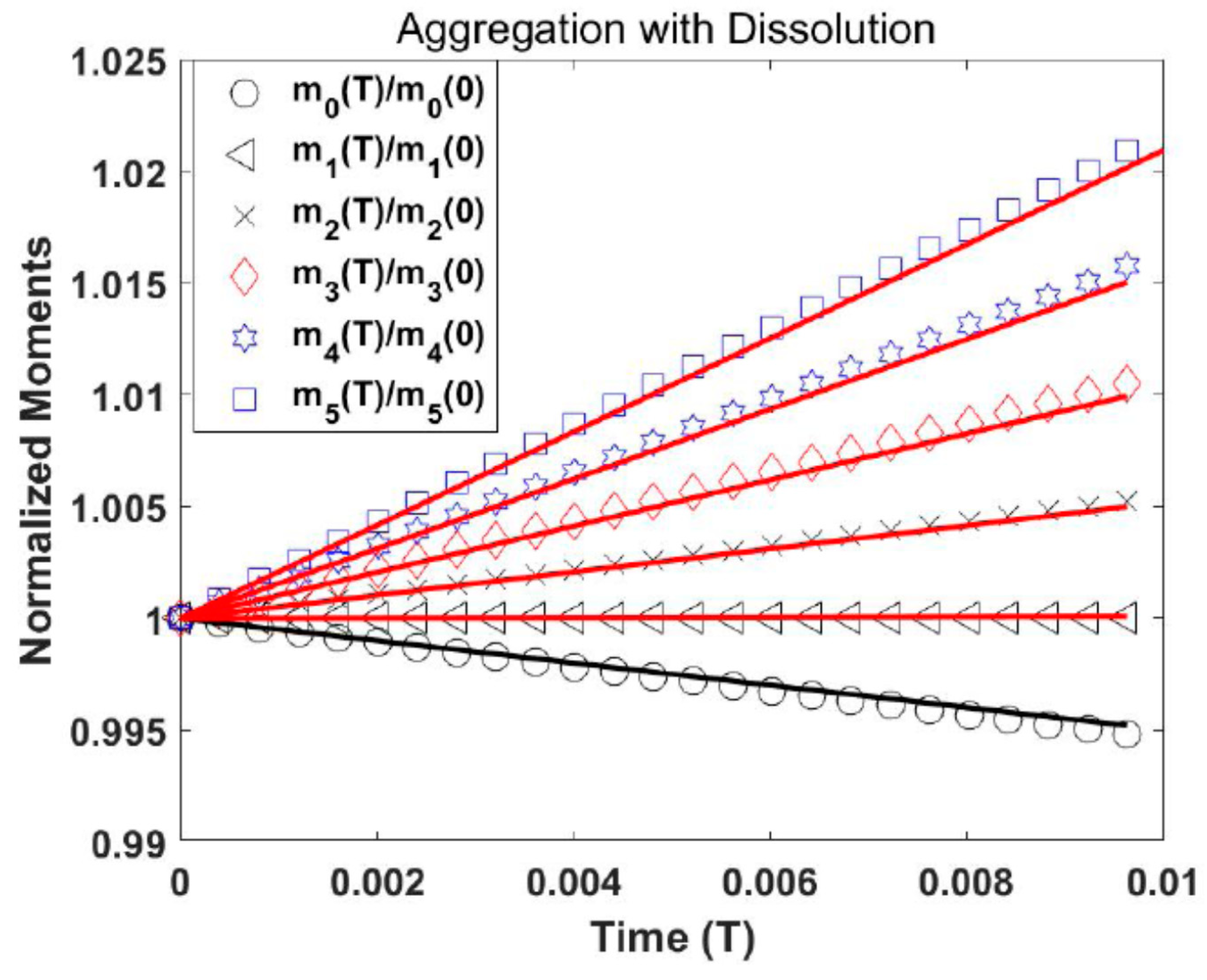
. The plot in
Figure 2 shows normalized moments. The outcomes of our QMOM are in decent agreement with analytical outcomes. It is also observed from
Figure 2 that during the aggregation process, the number of particles
decreases while the volume of the particles
remains constant.
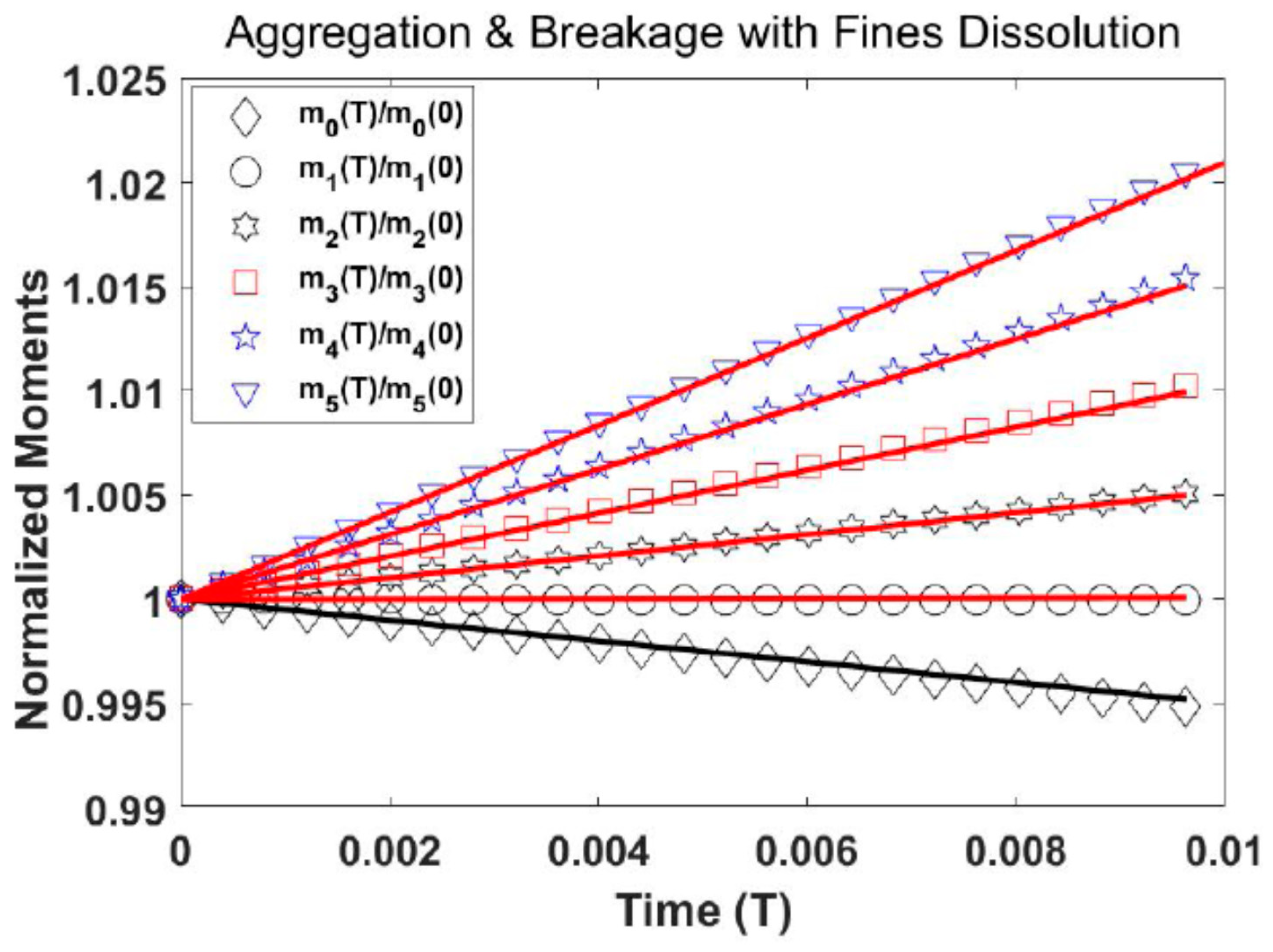
Test Problem 2: Aggregation and Breakage with Fines Dissolution
In this problem, we take a batch crystallizer in which aggregation and breakage are the main occurrences and which is connected with a fines dissolver. The growth and nucleation terms are neglected in this process. The initial distribution is given by
where,
and
represent the zero and first moments, respectively. A constant aggregation term,
a breakage kernel
, and uniform daughter distribution
are taken. The analytical solution is given by Patel [
17]:
The numerical results are displayed in
Figure 3. The moments of the numerical system are in good agreement with those taken from the analytical solution. It is also observed from
Figure 3 that during the aggregation and breakage process, the number of particles
decreases while the volume of the particles
remains constant.
