Mathematical Modelling Forecast on the Idling Transient Characteristic of Reactor Coolant Pump

 , ,
, ,
Abstract
:1. Introduction
2. Materials and Methods
2.1. Basic Theory of the Idling Condition of the Reactor Coolant Pump
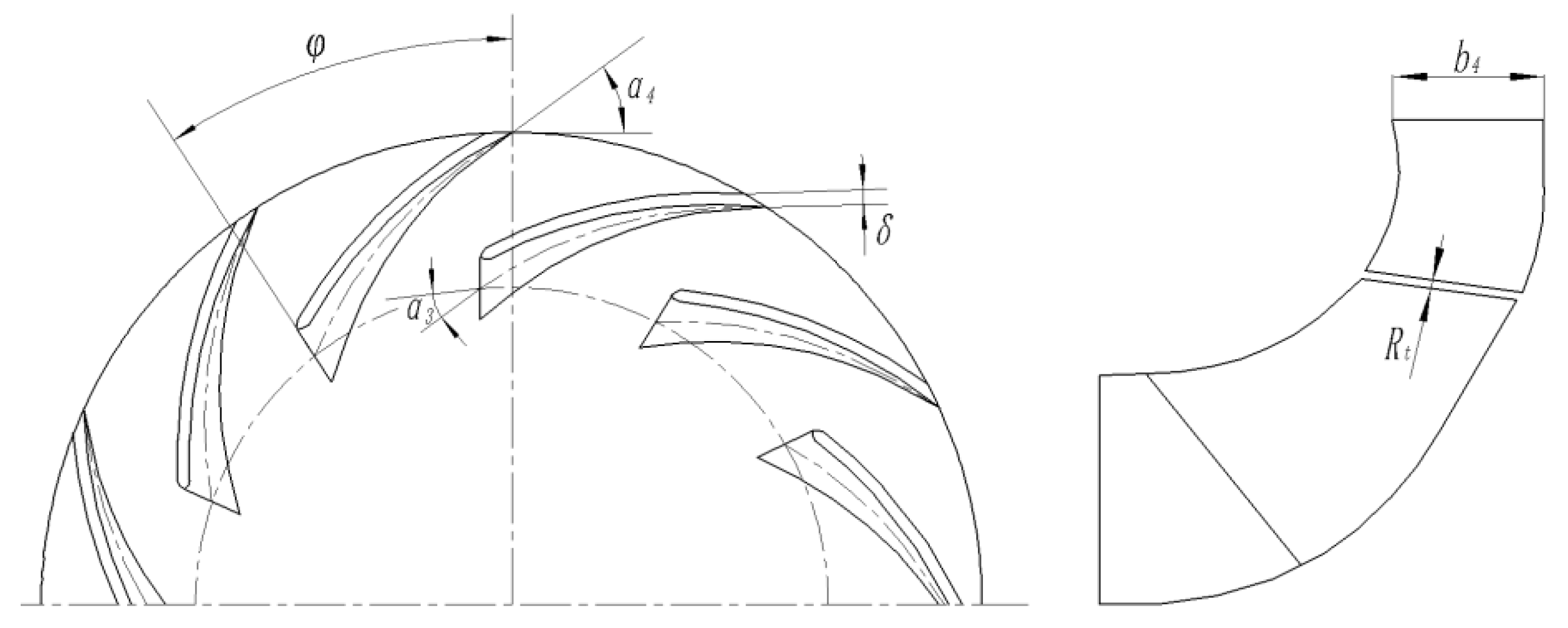
2.2. Hydraulic Modeling Database Construction on an Orthogonal Optimization Scheme
2.3. Mathematics Modeling Under Multiple Linear Regression Frameworks
3. Results
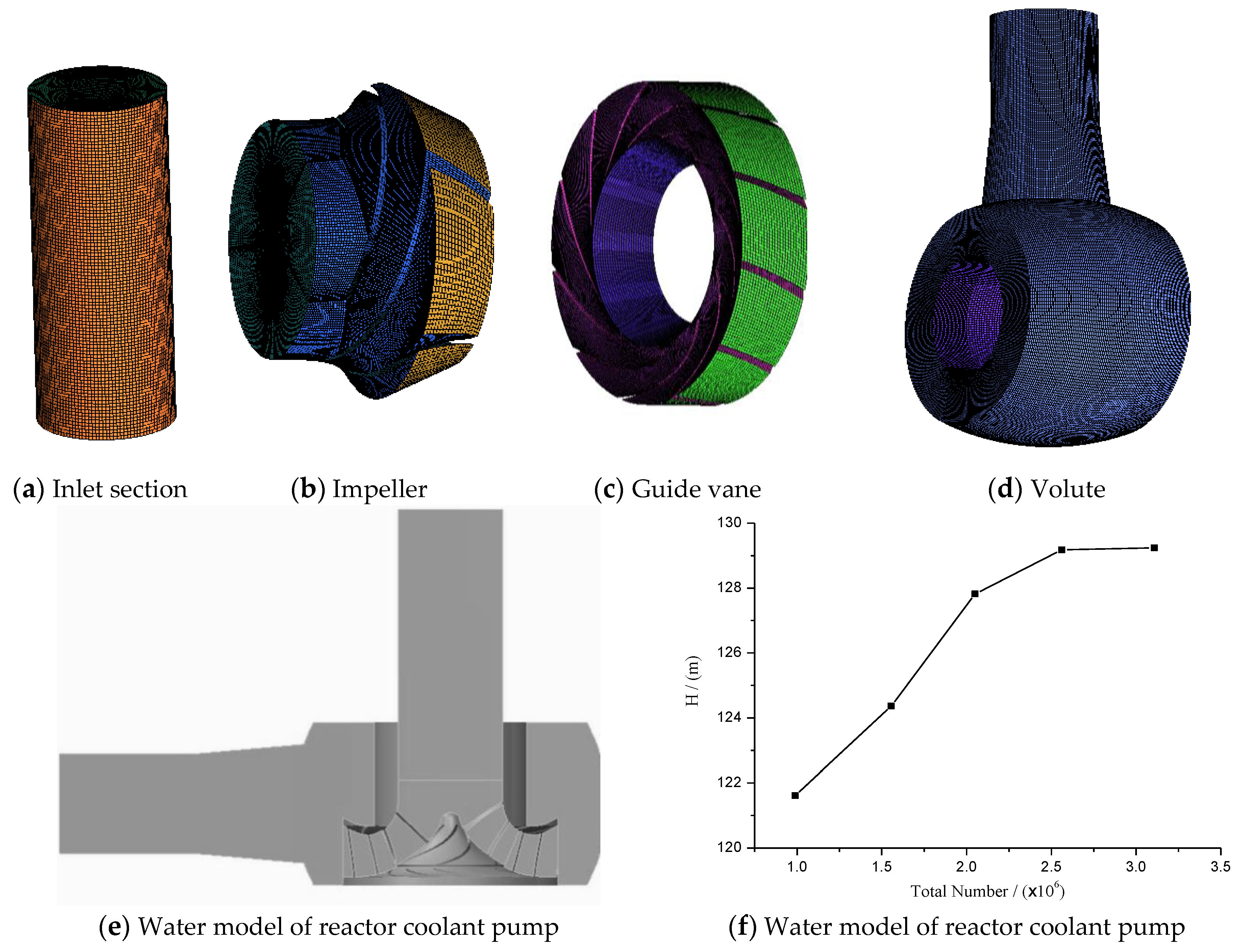
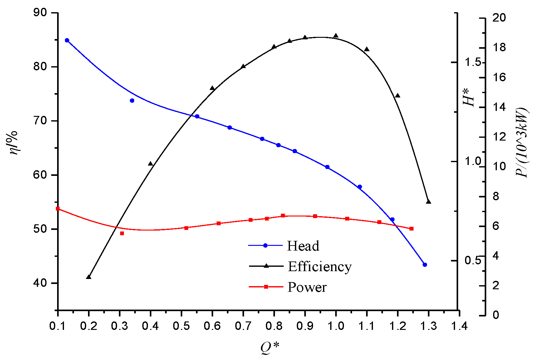
3.1. Solution of a Mathematical Model of Hydraulic Performance Based on MATLAB
- Load (‘efficiency.txt’);% read the work table file of efficiency.txt;
- a = load (‘efficiency.txt’);% assign the value of efficiency.txt to the contents a matrix;
- x1=a (:, 2);% assigns the value of the second column of a matrix to x1;
- x2=a (:, 3);% assigns the value of the third column of a matrix to x2;
- x3=a (:, 4);% assigns the value of the fourth column of a matrix to x3;
- x4=a (:, 5);% assigns the value of the Fifth column of a matrix to x1;
- x5=a (:, 6);% assigns the value of the sixth column of a matrix to x4;
- x6=a (:, 7);% assigns the value of the seventh column of a matrix to x5;
- y=a (:, 8);% assigns the value of the eighth column of a matrix to x6;
- X = [ones (length (y), 1), x1, x2, x3, x4, x5, x6];
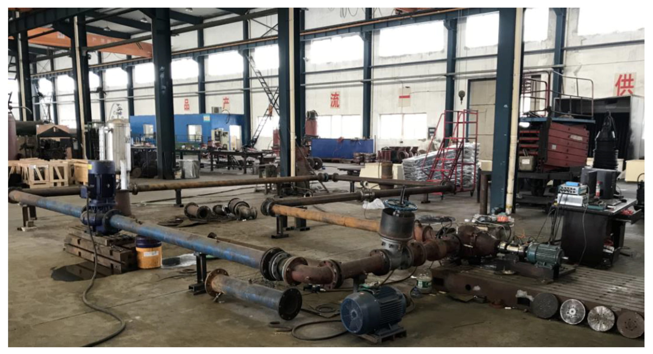
3.2. Test System of Reactor Coolant Pump Coasting
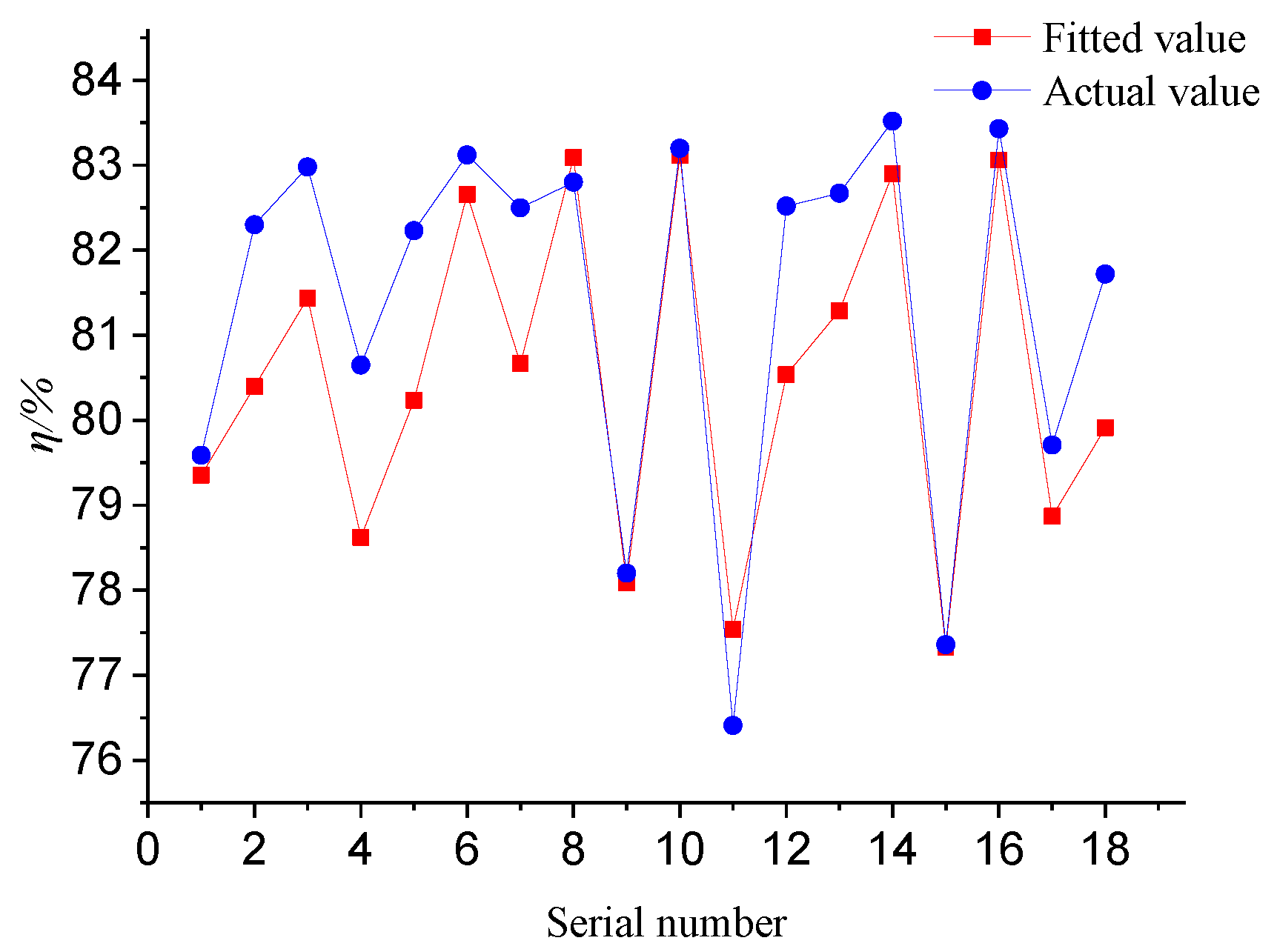
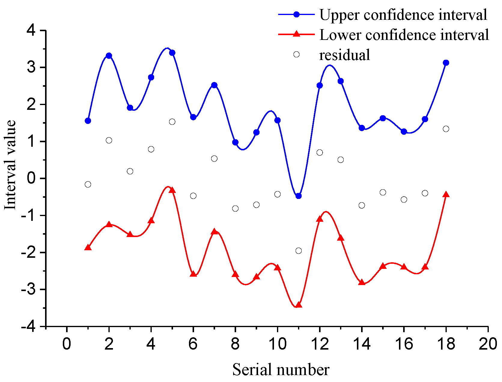
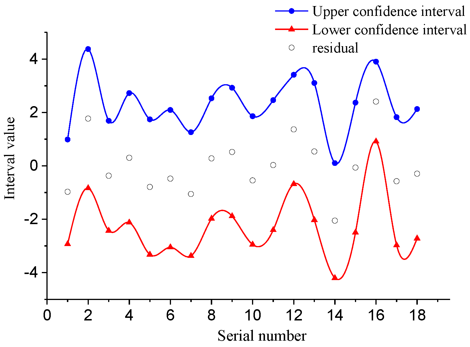
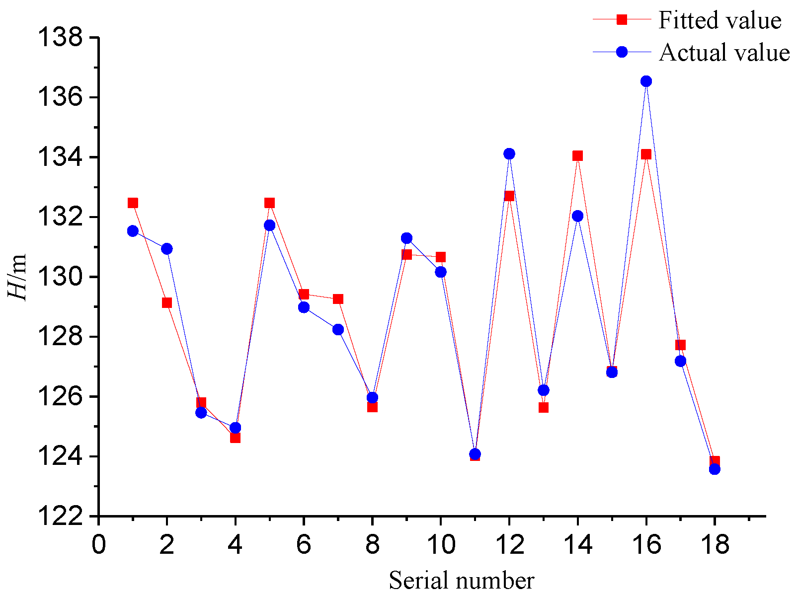
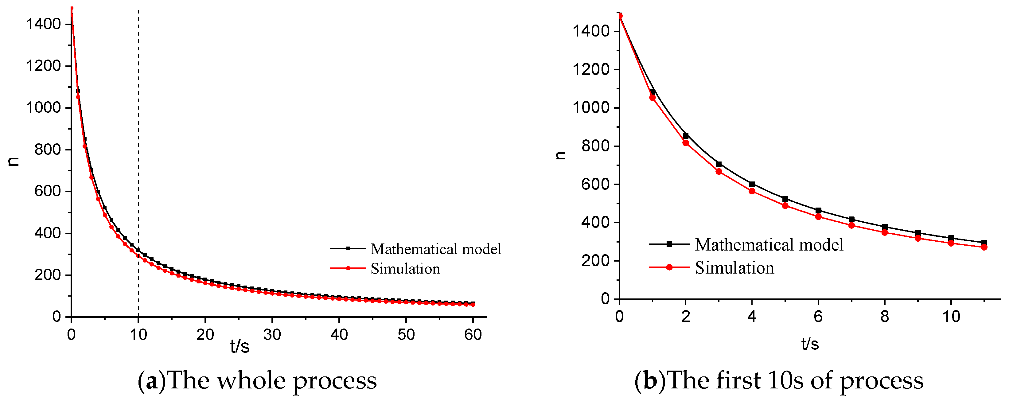
3.3. Verification of Mathematical Models
4. Conclusions
Author Contributions
Funding
Conflicts of Interest
References
- Sun, H. Third Generation Nuclear Power Technology AP1000, 2nd ed.; China Electric Power Press: Beijing, China, 2016. [Google Scholar]
- Yanjun, W.; Wenhong, L.; Jun, D.; Ling, G. Comparison of past and present the Chernobyl and the Fukushima nuclear accident and elicit thinking. Chin. J. Radiol. Health 2016, 25, 459–462. [Google Scholar]
- Dien, L.; Diep, D. Verification of VVER-1200 NPP simulator in normal operation and reactor coolant pump coast-down transient. World J. Eng. Technol. 2017, 5, 507–519. [Google Scholar] [CrossRef]
- Turnbull, B. RELAP5/MOD3.3 analysis of the reactor coolant pump trip event at NPP Krško for different transient scenarios. In Proceedings of the International Conference Nuclear Energy for New Europe 2005, Bled, Slovenia, 5–8 September 2005. [Google Scholar]
- Senru, Z. Calculation of transient characteristics for main circulating pump. Nuclear Power Eng. 1993, 2, 183–190. [Google Scholar]
- Yujun, G.; Jinling, Z.; Huizheng, Q.; Guanghui, S.; Dounan, J.; Zhenwan, Y. Calculating model of coolant pump flow characteristics for reactor system. Nucl. Sci. Eng. 1995, 3, 220–225, 231. [Google Scholar]
- Shaowen, D. Transient calculation of main pump in Qinshan Nuclear Power Plant Phase Two Project. Nucl. Power Eng. 2001, 6, 494–496, 507. [Google Scholar]
- Xu, Y. Numerical Simulation of Interior Flow Field of Reactor Coolant Pump Under Station Blackout Accident; Dalian University of Technology: Dalian, China, 2011. [Google Scholar]
- Zhu, R.; Long, Y.; Fu, Q.; Yuan, S.; Wang, X. Pressure fluctuation characteristics of nuclear main pump under low flow conditions. J. Vibr. Shock 2014, 33, 143–149. [Google Scholar]
- Yun, L.; Zhu, R.; Fu, Q.; Yuan, S.; Xi, Y. Numerical analysis on unstable flow of reactor coolant pump under small flow rate condition. J. Drain. Irrig. Eng. 2014, 32, 290–295. [Google Scholar]
- Feng, X.; Wu, D.; Yang, L.; Jia, Y. CNP1000 shaft seal reactor coolant pump technology. J. Drain. Irrig. Mach. Eng. 2016, 34, 553–560. [Google Scholar]
- Alatrash, Y.; Kang, H.O.; Yoon, H.G.; Seo, K.; Chi, D.Y.; Yoon, J. Experimental and analytical investigations of primary coolant pump coastdown phenomena for the Jordan Research and Training Reactor. Nucl. Eng. Des. 2015, 286, 60–66. [Google Scholar] [CrossRef]
- Brady, D.R.; Loebig, T.G. Reactor Coolant Pump Motor Load-Bearing Assembly Configuration. U.S. Patent No. 9,273,694, 1 March 2016. [Google Scholar]
- Bang, S.Y.; Chu, S.M.; Chang, J.Y. Development of Reactor Coolant Pump for APR1400. In Proceedings of the KNS 2015 Fall Meeting, Kyungju, Korea, 28–30 October 2015. [Google Scholar]
- Metzroth, K.; Denning, R.; Aldemir, T. Dynamic Event Tree Modeling of a Reactor Coolant Pump Seal LOCA. Adv. Conc. Nucl. Energy Risk Assess. Manag. 2018, 1, 305. [Google Scholar]
- Lu, Y.; Zhu, R.; Fu, Q.; Fu, Q.; An, C.; Chen, J. Research on the structure design of the LBE reactor coolant pump in the lead base heap. Nucl. Eng. Technol. 2019, 51, 546–555. [Google Scholar] [CrossRef]
- Lu, Y.; Zhu, R.; Wang, X.; Yang, W.; Qiang, F.; Daoxing, Y. Study on the complete rotational characteristic of coolant pump in the gas-liquid two-phase operating condition. Ann. Nucl. Energy 2019, 123, 180–189. [Google Scholar]
- Lu, Y.; Zhu, R.; Wang, X.; An, C.; Zhao, Y.; Fu, Q. Experimental study on transient performance in the coasting transition process of shutdown for reactor coolant pump. Nucl. Eng. Des. 2019, 346, 192–199. [Google Scholar] [CrossRef]


| Level | Factor | |||||
|---|---|---|---|---|---|---|
| α3/(°) | α4/(°) | φ/(°) | δ/mm | Rt/mm | b4/mm | |
| 1 | 22 | 20 | 70 | 10 | 5 | 280 |
| 2 | 26 | 25 | 75 | 20 | 15 | 290 |
| 3 | 30 | 30 | 80 | 30 | 25 | 300 |
| Serial Number | α3/° | α4/° | φ/° | δ/mm | Rt/mm | b4/mm | Indicator | |
|---|---|---|---|---|---|---|---|---|
| η/% | H/m | |||||||
| 1 | 22 | 18 | 70 | 15 | 5 | 280 | 79.59 | 131.532 |
| 2 | 22 | 20 | 75 | 20 | 10 | 290 | 82.30 | 130.936 |
| 3 | 22 | 22 | 80 | 25 | 15 | 300 | 82.98 | 125.46 |
| 4 | 26 | 18 | 70 | 20 | 15 | 300 | 80.65 | 124.954 |
| 5 | 26 | 20 | 75 | 25 | 5 | 280 | 82.23 | 131.721 |
| 6 | 26 | 22 | 80 | 15 | 10 | 290 | 83.12 | 128.98 |
| 7 | 30 | 18 | 75 | 25 | 10 | 300 | 82.50 | 128.234 |
| 8 | 30 | 20 | 80 | 15 | 15 | 280 | 82.80 | 125.961 |
| 9 | 30 | 22 | 70 | 20 | 5 | 290 | 78.20 | 131.295 |
| 10 | 22 | 18 | 80 | 20 | 10 | 280 | 83.20 | 130.161 |
| 11 | 22 | 20 | 70 | 25 | 15 | 290 | 76.41 | 124.076 |
| 12 | 22 | 22 | 75 | 15 | 5 | 300 | 82.52 | 134.112 |
| 13 | 26 | 18 | 75 | 15 | 15 | 290 | 82.67 | 126.207 |
| 14 | 26 | 20 | 80 | 20 | 5 | 300 | 83.52 | 132.032 |
| 15 | 26 | 22 | 70 | 25 | 10 | 280 | 77.36 | 126.807 |
| 16 | 30 | 18 | 80 | 25 | 5 | 290 | 83.43 | 136.537 |
| 17 | 30 | 20 | 70 | 15 | 10 | 300 | 79.71 | 127.18 |
| 18 | 30 | 22 | 75 | 20 | 15 | 280 | 81.72 | 123.568 |
| Value | bint | t | p | |
|---|---|---|---|---|
| b0 | 42.0264 | [17.3924,66.6604] | 3.5802 | 0.005 |
| b1 | 0.0283 | [−0.1473,0.2040] | 0.3385 | 0.742 |
| b2 | −0.2558 | [−0.6072,0.0955] | −1.5280 | 0.1575 |
| b3 | 0.4522 | [0.3116,0.5927] | 6.7517 | 0.501 |
| b4 | −0.0917 | [−0.2322,0.0489] | −1.3688 | 0.201 |
| b5 | −0.0377 | [−0.1782,0.1029] | −0.5624 | 0.5862 |
| b6 | 0.0415 | [−0.0288,0.1118] | 1.2394 | 0.0008 |
| bi | Value | bint |
|---|---|---|
| b0 | 54.061 | [39.9724,68.1503] |
| b1 | 0.0273 | [−0.1505,0.2072] |
| b2 | −0.256 | [−0.6135,0.1018] |
| b3 | 0.441 | [0.3091,0.5952] |
| b4 | −0.092 | [−0.2347,0.0514] |
| b5 | −0.038 | [−0.1807,0.1054] |
| bi | bint | |
|---|---|---|
| b0 | 123.176 | [93.5186,152.8324] |
| b1 | −0.073 | [−0.2845,0.1385] |
| b2 | −0.3085 | [−0.7315,0.1145] |
| b3 | 0.221 | [0.0523,0.3906] |
| b4 | −0.0189 | [−0.1881,0.1502] |
| b5 | −0.783 | [−0.9523,-0.6142] |
| b6 | 0.0185 | [−0.0661,0.1031] |
| Parameter | α3/° | α4/° | φ/° | δ/mm | Rt/mm | b4/mm |
|---|---|---|---|---|---|---|
| Value | 24 | 18 | 78 | 22 | 6 | 296 |
© 2019 by the authors. Licensee MDPI, Basel, Switzerland. This article is an open access article distributed under the terms and conditions of the Creative Commons Attribution (CC BY) license (http://creativecommons.org/licenses/by/4.0/).
Share and Cite
Wang, X.; Xie, Y.; Lu, Y.; Zhu, R.; Fu, Q.; Cai, Z.; An, C. Mathematical Modelling Forecast on the Idling Transient Characteristic of Reactor Coolant Pump. Processes 2019, 7, 452. https://doi.org/10.3390/pr7070452
Wang X, Xie Y, Lu Y, Zhu R, Fu Q, Cai Z, An C. Mathematical Modelling Forecast on the Idling Transient Characteristic of Reactor Coolant Pump. Processes. 2019; 7(7):452. https://doi.org/10.3390/pr7070452
Chicago/Turabian StyleWang, Xiuli, Yajie Xie, Yonggang Lu, Rongsheng Zhu, Qiang Fu, Zheng Cai, and Ce An. 2019. "Mathematical Modelling Forecast on the Idling Transient Characteristic of Reactor Coolant Pump" Processes 7, no. 7: 452. https://doi.org/10.3390/pr7070452
APA StyleWang, X., Xie, Y., Lu, Y., Zhu, R., Fu, Q., Cai, Z., & An, C. (2019). Mathematical Modelling Forecast on the Idling Transient Characteristic of Reactor Coolant Pump. Processes, 7(7), 452. https://doi.org/10.3390/pr7070452