Irregularity Molecular Descriptors of Hourglass, Jagged-Rectangle, and Triangular Benzenoid Systems

Abstract

Determining the degree of irregularity of a certain molecular structure or a network has been a key source of interest for molecular topologists, but it is also important as it provides an insight into the key features used to guess properties of the structures. In this article, we are interested in formulating closed forms of irregularity measures of some popular benzenoid systems, such as hourglass H (m, n), jagged-rectangular J (m, n), and triangular benzenoid T (m, n) systems. We also compared our results graphically and concluded which benzenoid system among the above listed is more irregular than the others.

1. Introduction

Benzenoid hydrocarbons have consistently attracted the attention of both chemists and pure mathematicians because of the complexities of the underlying molecular graphs, combinatorically and topologically. Research in benzenoid hydrocarbons is currently expanding due to innovative developments. Benzenoid systems are molecular structures that have nice geometrical properties. These systems are connected, infinite chains of concatenated benzenes with the property of two adjacent benzenes having a single common edge. These are constructed with a definite rule from a benzene molecule, which happens to be its fundamental building block. A benzenoid system is defined to be a connected planar simple graph obtained by regular hexagons, with two such hexagons sharing a common edge or disjoint. All benzenoid systems partition the plane into one non-compact external region and many internal compact regular hexagonal regions. Let h be the number of hexagons in a benzenoid system, then, for h = 1, we have a single, non-isomorphic benzenoid system as the single benzene molecule. For h = 2, 3, and 4, we obtain the number following non-isomorphic benzenoid systems in Figure 1 ([1] pp. 11–15).

For h = 1 we have a single hexagonal cycle and, for h = 2, we have a unique, non-isomorphic structure. Mathematical chemistry can be useful to predict the properties of chemical compounds without the help of quantum mechanics. Key tools used to carry such information are polynomials and numbers, which collectively gather information relating to the pattern and topology of the molecular graph. The co-relation of various physical properties like standard enthalpy of vaporization, boiling point, entropy and heat of vaporization, as well as reactivity and biological mechanics, are theoretically based on these tools. Some connections of the physical properties of molecules with topological indices have been given in [2,3,4]. Estrada established a connection between the atom bond connectivity index and energies of the branched alkanes in [5]. Applications of some indices in pharmacology have been given in [6] and in structure–activity analysis in [7,8].

The subject matter of the present article is some well-known benzenoid systems. These are molecular graphs comprising of the arrangements of carbon atoms with depleted hydrogen. It has been keenly observed that the geometry and pattern of benzene in the system characterize its physical aspects [1,5,6]. These graphs consist of one infinite (outer) region and a number of finite (inner) regions. All internal regions must be regular hexagons. The vertex of a hexagonal system belongs to, at most, three hexagons. A vertex shared by three hexagons is called an internal vertex. Benzenoid systems are of great importance in theoretical chemistry and, as so, are recently well-studied [9,10,11]. Kwun et al. computed M-polynomials for triangular, hourglass, and jagged rectangle benzenoid systems, and from these M-polynomials, they recovered nine degree-based topological indices in [9]. In [10,11,12], the authors computed some degree-based indices and polynomials of benzenoid systems. For computational aspects and analysis of different degree-based indices of some famous tubes and nanomaterials, see [12,13,14,15].

In this article, we are interested in the characteristic study of irregularity determinants of some famous benzenoid systems, namely, triangular, hourglass, and jagged-rectangular benzenoid systems.

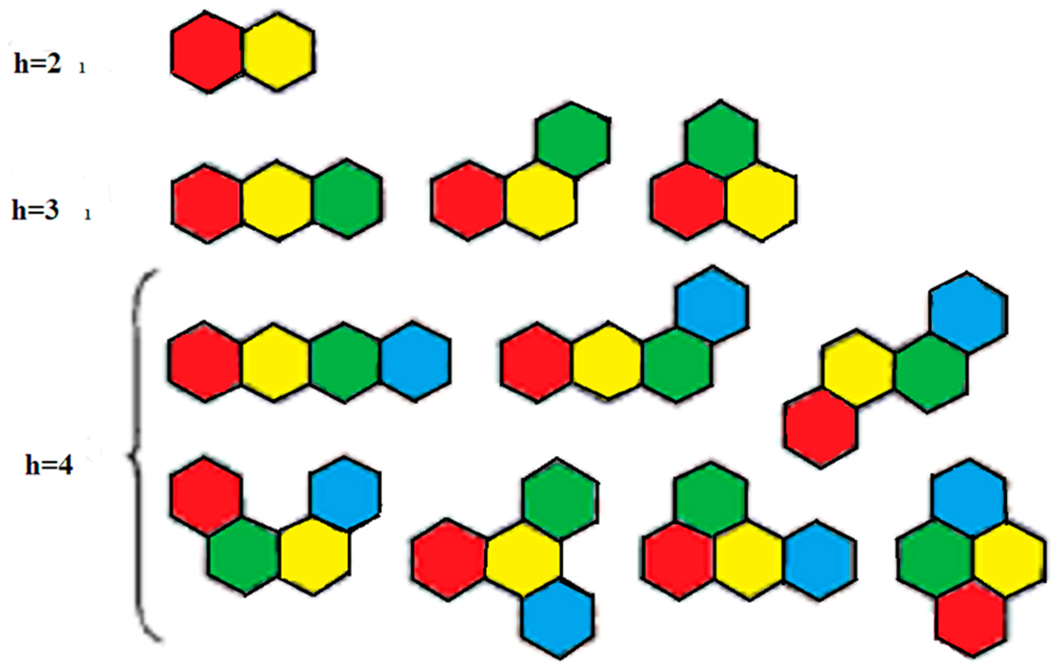
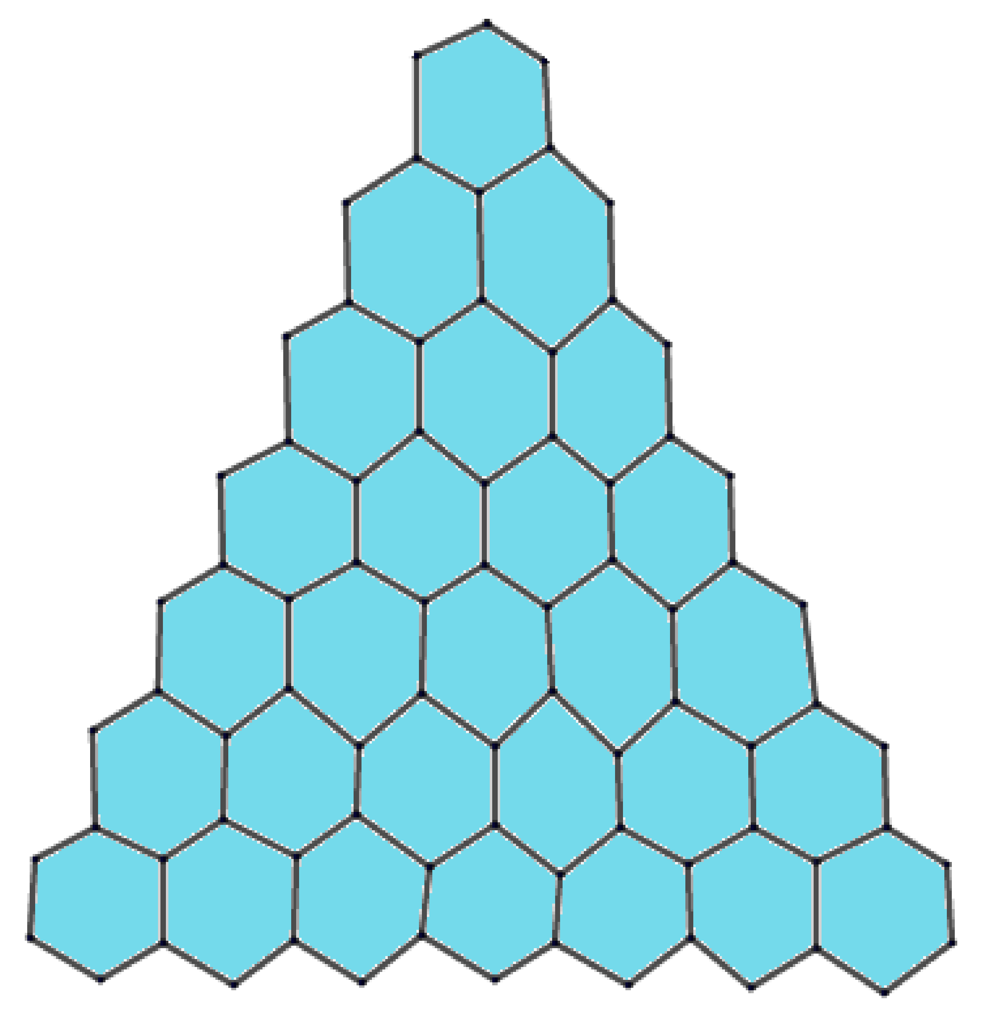
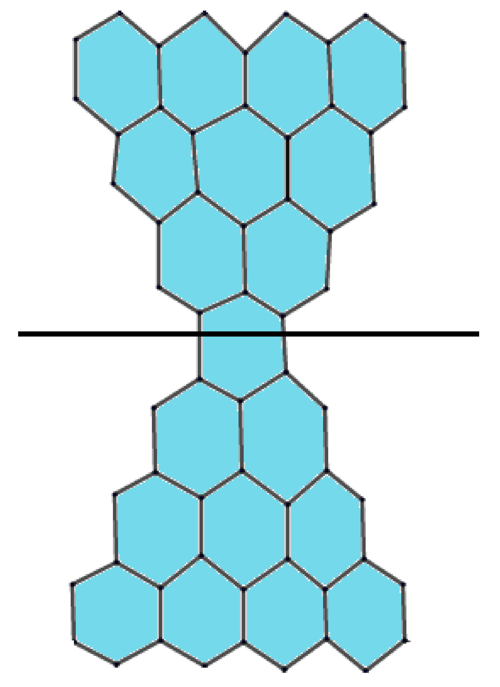
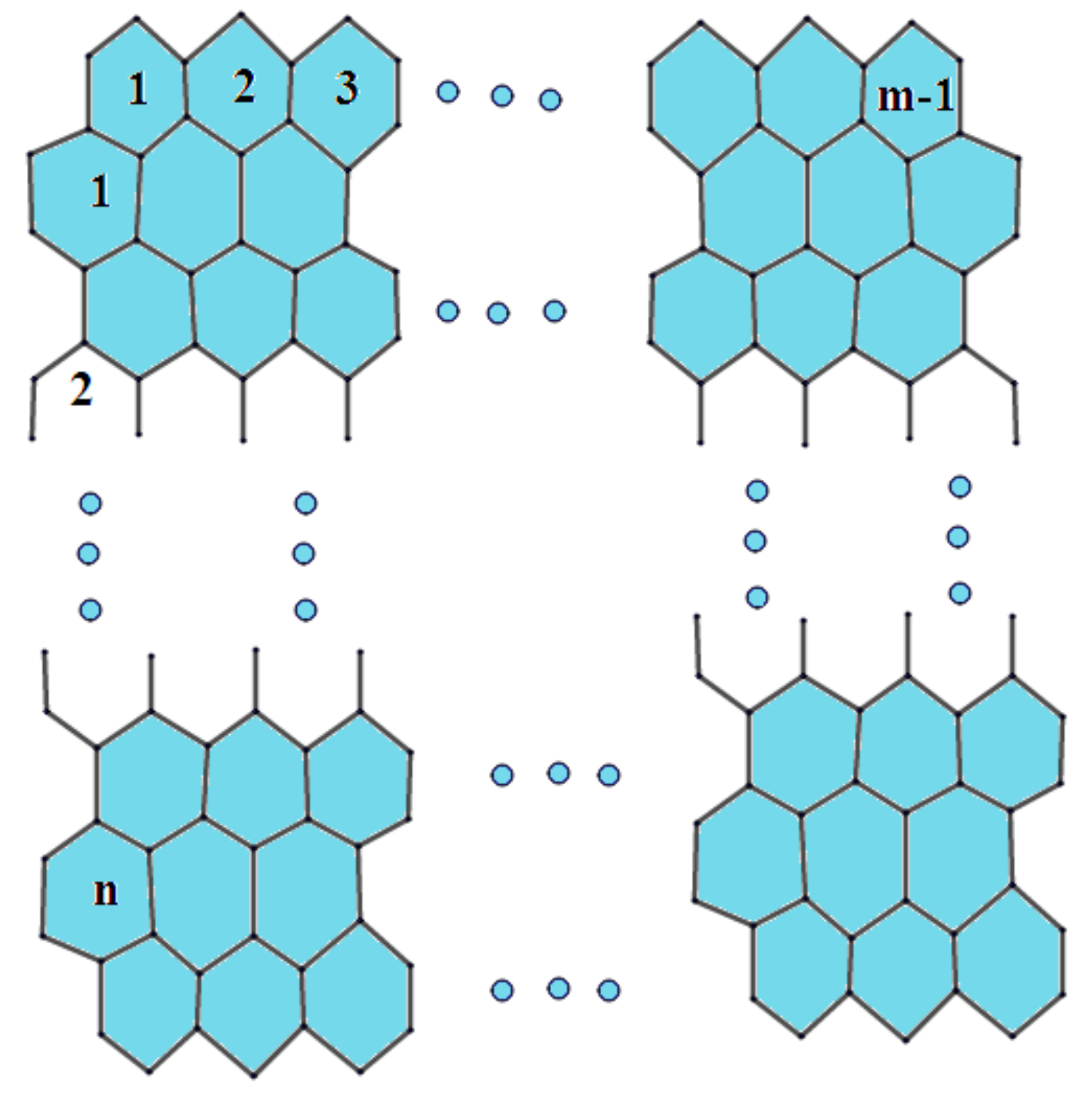
2. Preliminaries and Notations

Let G be a simple connected graph with vertex V, edge set E, du and dv the degree of vertices u and v. A topological invariant is an isomorphism of the graph that preserves the topology of the graph. A graph is said to be regular if every vertex of the graph has the same degree. A topological invariant is called an irregularity index if this index vanishes for a regular graph, and is non-zero for a non-regular graph. Regular graphs have been extensively investigated, particularly in mathematics. Their applications in chemical graph theory came to be known after the discovery of nanotubes and fullerenes. Paul Erdos emphasized this in the study of irregular graphs for the first time in history in [16]. In the Second Krakow Conference on Graph Theory (1994), Erdos officially posed it as an open problem, ‘’The determination of extreme size of highly irregular graphs of given order”, [17]. Since then, irregular graphs and the degree of irregularity have become one of the core open problems of graph theory. A graph in which each vertex has a different degree then the other vertices is known as a perfect graph. The authors of [18] demonstrated that no graph is perfect. The graphs lying in between are called quasi-perfect graphs, in which all except two vertices have different degrees [17]. Simplified ways of expressing the irregularities are irregularity indices. These irregularity indices have been studied recently in a novel way [19,20]. The first such irregularity index was introduced in [21]. Most of these indices used the concept of the imbalance of an edge defined as $imbal{l}_{uv}=\left|du-dv\right|$, [22,23]. The Albertson index, AL(G), was defined by Alberston in [23] as $AL\left(G\right)={{\displaystyle \sum }}_{UV\in E}\left|d_u-d_v\right|$. In this index, the imbalance of edges are computed. The irregularity index IRL(G) and IRLU(G) is introduced by Vukicevic and Gasparov, [24] as $IRL\left(G\right)={{\displaystyle \sum }}_{UV\in E}\left|ln{d}_u-ln{d}_v\right|$, and $IRLU\left(G\right)={{\displaystyle \sum }}_{UV\in E}\frac{\left|d_u-d_v\right|}{min\left(d_u,d_v\right)}$. Recently, Abdoo et al. introduced the new term “total irregularity measure of a graph G”, which is defined as [25,26,27] $IR{R}_t\left(G\right)=\frac{1}{2}{{\displaystyle \sum }}_{UV\in E}\left|d_u-d_v\right|$. Recently, Gutman et al. introduced the IRF(G) irregularity index of the graph G, which is described as $IRF\left(G\right)={{\displaystyle \sum }}_{UV\in E}{\left(d_u-d_v\right)}^2$ in [28]. The Randic index itself is directly related to an irregularity measure, which is described as $IRA\left(G\right)={{\displaystyle \sum }}_{UV\in E}{\left(d_u^{\raisebox{1ex}{$-1$}\!\left/ \!\raisebox{-1ex}{$2$}\right.}-d_v^{\raisebox{1ex}{$-1$}\!\left/ \!\raisebox{-1ex}{$2$}\right.}\right)}^2$ in [29]. Further irregularity indices of similar nature can be traced in [29] in detail. These indices are given as $IRDIF\left(G\right)={{\displaystyle \sum }}_{UV\in E}\left|\frac{d_u}{d_v}-\frac{d_v}{d_v}\right|$, $IRLF\left(G\right)={{\displaystyle \sum }}_{UV\in E}\frac{\left|d_u-d_v\right|}{\sqrt{\left(d_u{d}_v\right)}}$, $LA\left(G\right)=2{{\displaystyle \sum }}_{UV\in E}\frac{\left|d_u-d_v\right|}{\left(d_u+d_v\right)}$, $IRD1={{\displaystyle \sum }}_{UV\in E}ln\left\{1+\left|d_v-d_v\right|\right\}$, $IRGA\left(G\right)={{\displaystyle \sum }}_{UV\in E}ln\frac{d_u+d_v}{2\sqrt{\left(d_u{d}_v\right)}}$, and $IRB\left(G\right)={{\displaystyle \sum }}_{UV\in E}{\left(d_u^{\raisebox{1ex}{$1$}\!\left/ \!\raisebox{-1ex}{$2$}\right.}-d_v^{\raisebox{1ex}{$1$}\!\left/ \!\raisebox{-1ex}{$2$}\right.}\right)}^2$. Further details can be given in [29,30,31,32,33,34,35,36,37,38,39,40]. Recently, Zahid et al. computed the irregularity indices of a nanotube [41]. Gao et al. recently computed irregularity measures of some dendrimer structures in [42] and molecular structures in [43]. These structures are used as long infinite chain macromolecules in chemistry and related areas.

In the current article, we are interested in finding the degree of irregularity of the triangular, hourglass, and jagged-rectangle benzenoid systems. Figure 2, Figure 3 and Figure 4 represent molecular graphs of these three systems. The main motivation comes from the fact that graphs of the irregularity indices show close accurate results about properties like entropy, standard enthalpy, vaporization, and acentric factors of octane isomers [29]. The molecular pattern and topology of these three benzenoid systems are shown in these figures. In Figure 2, benzenes increase by one, like a pyramid in T_m. In hourglass benzenoid systems, one central benzene exists and the number of benzenes increases by one in both upward and downward directions in Figure 3, whereas jagged-rectangular benzenoid systems are shown in Figure 4.

The horizontal line at the center is drawn just to indicate the line of symmetry of $H_m$.

3. Main Results

In this section, we present our main theoretical results.

Theorem 1.

Let $T_m$ be the triangular benzenoid system, then the irregularity indices of $T_m$ are:

1. 

$IRDIF\left(T_m\right)=3m-3$

2. 

$AL\left(T_m\right)=6m-6$

3. 

$IRL\left(T_m\right)=2.4329m-2.43279$

4. 

$IRLU\left(T_m\right)=3m-3$

5. 

$IRLU\left(T_m\right)=\sqrt{6}m-\sqrt{6}$

6. 

$IRF\left(T_m\right)=6m-6$

7. 

$IRLA\left(T_m\right)=\frac{12}{5}m-\frac{12}{5}$

8. 

$IRD1=4.15888m-4.15888308$

9. 

$IRA\left(T_m\right)=5-2\sqrt{6}m-5-2\sqrt{6}$

10. 

$IRGA\left(T_m\right)=0.1225m-0.122465$

11. 

$IRB\left(T_m\right)=30-12\sqrt{6}m-30-12\sqrt{6}$

12. 

$IR{R}_t\left(T_m\right)=3\left(m-1\right)$

Proof. 

In order to prove the above theorem, we have to consider Figure 2. Here, m is the number of hexagons in the last row of the triangular benzenoid system, and $\left|V\left(T_m\right)\right|=1+m^2+4m$ and $\left|E\left(T_m\right)\right|=\frac{3}{2}m\left(m+3\right)$. We can see that the edges of $T_m$ admit the following partition in

Table 1. Edge partition of triangular benzenoid system.

Number of Edges $({\mathit{d}}_{\mathit{u}},{\mathit{d}}_{\mathit{v}})$	Number of Indices
(2, 2)	$6$
(2, 3)	$6\left(m-1\right)$
(3, 3)	$\frac{3}{2}m\left(m-1\right)$

. □

Now using Table 1 and the above definitions, we have:

• $IRDIF\left(G\right)={{\displaystyle \sum }}_{UV\in E}\left|\frac{d_u}{d_v}-\frac{d_v}{d_v}\right|$

  $$\begin{array}{ll}IRDIF\left(T_m\right)& =6\left|\frac{2}{2}-\frac{2}{2}\right|+6\left(m-1\right)\left|\frac{3}{2}-\frac{2}{3}\right|+\frac{3}{2}m\left(m-1\right)\left|\frac{3}{3}-\frac{3}{3}\right|\\ & =3\left(m-1\right).\end{array}$$
• $AL\left(G\right)={{\displaystyle \sum }}_{UV\in E}\left|d_u-d_v\right|$

  $$\begin{array}{ll}AL\left(T_m\right)& =6\left|2-2\right|+6\left(m-1\right)\left|3-2\right|+\frac{3}{2}m\left(m-1\right)\left|3-3\right|\\ & =6\left(m-1\right).\end{array}$$
• $IRL\left(G\right)={{\displaystyle \sum }}_{UV\in E}\left|ln{d}_u-ln{d}_v\right|$

  $$\begin{array}{ll}IRL\left(T_m\right)& =6\left|ln2-ln2\right|+6\left(m-1\right)\left|ln3-ln2\right|+\frac{3}{2}m\left(m-1\right)\left|ln3-ln3\right|\\ & =6\left(m-1\right)\left|ln\frac{3}{2}\right|.\end{array}$$
• $IRLU\left(G\right)={{\displaystyle \sum }}_{UV\in E}\frac{\left|d_u-d_v\right|}{min\left(d_u{d}_v\right)}$

  $$\begin{array}{ll}IRLU\left(T_m\right)& =6\frac{\left|2-2\right|}{2}+6\left(m-1\right)\frac{\left|3-2\right|}{2}+\frac{3}{2}m\left(m-1\right)\frac{\left|3-3\right|}{2}\\ & =3\left(m-1\right).\end{array}$$
• $IRLF\left(G\right)={{\displaystyle \sum }}_{UV\in E}\frac{\left|d_u-d_v\right|}{\sqrt{\left(d_u{d}_v\right)}}$

  $$\begin{array}{ll}IRLF\left(T_m\right)& =6\frac{\left|2-2\right|}{\sqrt{\left(4\right)}}+6\left(m-1\right)\frac{\left|3-2\right|}{\sqrt{\left(6\right)}}+\frac{3}{2}m\left(m-1\right)\frac{\left|3-3\right|}{\sqrt{9}}\\ & =6\left(m-1\right)\frac{1}{\sqrt{\left(6\right)}}.\end{array}$$
• $IRF\left(G\right)={{\displaystyle \sum }}_{UV\in E}{\left(d_u-d_v\right)}^2$

  $$\begin{array}{ll}IRF\left(T_m\right)& =6{\left(2-2\right)}^2+6\left(m-1\right){\left(3-2\right)}^2+\frac{3}{2}m\left(m-1\right){\left(3-3\right)}^2\\ & =6\left(m-1\right).\end{array}$$
• $IRLA\left(G\right)=2{{\displaystyle \sum }}_{UV\in E}\frac{\left|d_u-d_v\right|}{\left(d_u+d_v\right)}$

  $$\begin{array}{ll}IRLA\left(T_m\right)& =2\left[6\frac{\left|2-2\right|}{\left(4\right)}+6\left(m-1\right)\frac{\left|3-2\right|}{\left(5\right)}+\frac{3}{2}m\left(m-1\right)\frac{\left|3-3\right|}{\left(5\right)}\right]\\ & =12\left(m-1\right)\frac{1}{\left(5\right)}.\end{array}$$
• $IRD1={{\displaystyle \sum }}_{UV\in E}ln\left\{1+\left|d_v-d_v\right|\right\}$

  $$\begin{array}{l}=6ln\left\{1+\left|2-2\right|\right\}+6\left(m-1\right)ln\left\{1+\left|3-2\right|\right\}+\frac{3}{2}m\left(m-1\right)ln\left\{1+\left|3-3\right|\right\}\\ =6\left(m-1\right)ln2.\end{array}$$
• $IRA\left(G\right)={{\displaystyle \sum }}_{UV\in E}{\left(d_u^{\raisebox{1ex}{$-1$}\!\left/ \!\raisebox{-1ex}{$2$}\right.}-d_v^{\raisebox{1ex}{$-1$}\!\left/ \!\raisebox{-1ex}{$2$}\right.}\right)}^2$

  $$\begin{array}{ll}IRA\left(T_m\right)& =6{\left(\frac{1}{\sqrt{2}}-\frac{1}{\sqrt{2}}\right)}^2+6\left(m-1\right){\left(\frac{1}{\sqrt{3}}-\frac{1}{\sqrt{2}}\right)}^2+\frac{3}{2}m\left(m-1\right){\left(\frac{1}{\sqrt{3}}-\frac{1}{\sqrt{3}}\right)}^2\\ & =6\left(m-1\right){\left(\frac{1}{\sqrt{3}}-\frac{1}{\sqrt{2}}\right)}^2.\end{array}$$
• $IRGA\left(G\right)={{\displaystyle \sum }}_{UV\in E}ln\frac{d_u+d_v}{2\sqrt{\left(d_u{d}_v\right)}}$

  $$\begin{array}{ll}IRGA\left(T_m\right)& =6ln\frac{2+2}{2\sqrt{\left(4\right)}}+6\left(m-1\right)ln\frac{3+2}{2\sqrt{\left(6\right)}}+\frac{3}{2}m\left(m-1\right)ln\frac{3+3}{2\sqrt{\left(9\right)}}\\ & =6\left(m-1\right)ln\frac{5}{2\sqrt{\left(6\right)}}.\end{array}$$
• $IRB\left(G\right)={{\displaystyle \sum }}_{UV\in E}{\left(d_u^{\raisebox{1ex}{$1$}\!\left/ \!\raisebox{-1ex}{$2$}\right.}-d_v^{\raisebox{1ex}{$1$}\!\left/ \!\raisebox{-1ex}{$2$}\right.}\right)}^2$

  $$\begin{array}{ll}IRB\left(T_m\right)& =6{\left(\sqrt{2}-\sqrt{2}\right)}^2+6\left(m-1\right){\left(\sqrt{3}-\sqrt{2}\right)}^2+\frac{3}{2}m\left(m-1\right){\left(\sqrt{3}-\sqrt{3}\right)}^2\\ & =6\left(m-1\right){\left(\sqrt{3}-\sqrt{2}\right)}^2.\end{array}$$
• $IR{R}_t\left(G\right)=\frac{1}{2}{{\displaystyle \sum }}_{UV\in E}\left|d_u-d_v\right|$

  $$\begin{array}{ll}IR{R}_t\left(T_m\right)& =\frac{1}{2}\left[6\left|2-2\right|+6\left(m-1\right)\left|3-2\right|+\frac{3}{2}m\left(m-1\right)\left|3-3\right|\right]\\ & =3\left(m-1\right).\end{array}$$

Table 2. Irregularity indices for triangular benzenoid system $T_m$.

Irregularity Indices	m = 1	m = 2	m = 3	m = 4	m = 5
$IRDIF\left(G\right)={{\displaystyle \sum }}_{UV\in E}\left|\frac{d_u}{d_v}-\frac{d_v}{d_v}\right|$	0	3	6	9	12
$AL\left(G\right)={{\displaystyle \sum }}_{UV\in E}\left|d_u-d_v\right|$	0	6	12	18	24
$IRL\left(G\right)={{\displaystyle \sum }}_{UV\in E}\left|ln{d}_u-ln{d}_v\right|$	0	2.4329	4.8658	7.2987	9.7316
$IRLU\left(G\right)={{\displaystyle \sum }}_{UV\in E}\frac{\left|d_u-d_v\right|}{min\left(d_u,d_v\right)}$	0	3	6	9	12
$IRLU\left(G\right)={{\displaystyle \sum }}_{UV\in E}\frac{\left|d_u-d_v\right|}{\sqrt{\left(d_u{d}_v\right)}}$	0	2.44949	4.89898	7.34847	9.79796
$IRF\left(G\right)={{\displaystyle \sum }}_{UV\in E}{\left(d_u-d_v\right)}^2$	0	6	12	18	24
$IRLA\left(G\right)=2{{\displaystyle \sum }}_{UV\in E}\frac{\left|d_u-d_v\right|}{\left(d_u+d_v\right)}$	0	2.40	4.80	7.20	9.60
$IRD1={{\displaystyle \sum }}_{UV\in E}ln\left\{1+\left|d_v-d_v\right|\right\}$	0	4.15888	8.31776	12.47664	16.63552
$IRA\left(G\right)={{\displaystyle \sum }}_{UV\in E}{\left(d_u^{\raisebox{1ex}{$-1$}\!\left/ \!\raisebox{-1ex}{$2$}\right.}-d_v^{\raisebox{1ex}{$-1$}\!\left/ \!\raisebox{-1ex}{$2$}\right.}\right)}^2$	0	0.101022	0.202044	0.303066	0.404088
$IRGA\left(G\right)={{\displaystyle \sum }}_{UV\in E}ln\frac{d_u+d_v}{2\sqrt{\left(d_u{d}_v\right)}}$	0	0.122465	0.244930	0.367395	0.489860
$IRB\left(G\right)={{\displaystyle \sum }}_{UV\in E}{\left(d_u^{\raisebox{1ex}{$1$}\!\left/ \!\raisebox{-1ex}{$2$}\right.}-d_v^{\raisebox{1ex}{$1$}\!\left/ \!\raisebox{-1ex}{$2$}\right.}\right)}^2$	0	0.60612	1.21224	1.81836	2.42448
$IR{R}_t\left(G\right)=\frac{1}{2}{{\displaystyle \sum }}_{UV\in E}\left|d_u-d_v\right|$	0	3	6	9	12

. shows the values of these irregularity indices for some test values of parameter m.

Theorem 2.

Let $H_m$ be the hourglass benzenoid system, then the irregularity indices of $H_m$ are:

1. 

$IRDIF\left(H_m\right)=6m-8$

2. 

$AL\left(H_m\right)=12m-16$

3. 

$IRL\left(H_m\right)=4.86559m-6.48745$

4. 

$IRLU\left(H_m\right)=6m-8$

5. 

$IRLU\left(H_m\right)=2\sqrt{6}m-\frac{32\sqrt{6}}{3}$

6. 

$IRF\left(H_m\right)=12m-16$

7. 

$IRLA\left(H_m\right)=\frac{24}{5}m-\frac{32}{5}$

8. 

$IRD1=8.31776m-11.09035489$

9. 

$IRA\left(H_m\right)=10-4\sqrt{6}m-\frac{40-16\sqrt{6}}{3}$

10. 

$IRGA\left(H_m\right)=0.245m-0.32658$

11. 

$IRB\left(H_m\right)=60-24\sqrt{6}m-80-32\sqrt{6}$

12. 

$IR{R}_t\left(H_m\right)=2\left(3m-4\right)$

Proof. 

In order to prove the above theorem, we have to consider Figure 3. Here, $H_m$ indicates the hourglass benzenoid system which is acquired from the two duplicates of triangular benzenoid system $T_m$ by overlapping their exterior hexagons. Then, we have $\left|V(H_m)\right|=2\left(m^2+4m-2\right)$ and $\left|E(H_m)\right|=3m^2+9m-4$. We can see that the edges of $H_m$ admit the following partition in

Table 3. Edge partition of hourglass benzenoid system.

Number of Edges $({\mathit{d}}_{\mathit{u}},{\mathit{d}}_{\mathit{v}})$	Number of Indices
(2, 2)	$8$
(2, 3)	$4\left(3m-4\right)$
(3, 3)	$\left(3m^2-3m+4\right)$

. □

Now using above Table 3, and the above definitions, we have:

• $IRDIF\left(G\right)={{\displaystyle \sum }}_{UV\in E}\left|\frac{d_u}{d_v}-\frac{d_v}{d_v}\right|$

  $$\begin{array}{ll}IRDIF\left(H_m\right)& =8\left|\frac{2}{2}-\frac{2}{2}\right|+4\left(3m-4\right)\left|\frac{3}{2}-\frac{2}{3}\right|+\left(3m^2-3m+4\right)\left|\frac{3}{3}-\frac{3}{3}\right|\\ & =2\left(3m-4\right).\end{array}$$
• $AL\left(G\right)={{\displaystyle \sum }}_{UV\in E}\left|d_u-d_v\right|$

  $$\begin{array}{ll}AL\left(H_m\right)& =8\left|2-2\right|+4\left(3m-4\right)\left|3-2\right|+\left(3m^2-3m+4\right)\left|3-3\right|\\ & =4\left(3m-4\right).\end{array}$$
• $IRL\left(G\right)={{\displaystyle \sum }}_{UV\in E}\left|ln{d}_u-ln{d}_v\right|$

  $$\begin{array}{ll}IRL\left(H_m\right)& =8\left|ln2-ln2\right|+4\left(3m-4\right)\left|ln3-ln2\right|+\left(3m^2-3m+4\right)\left|ln3-ln3\right|\\ & =4\left(3m-4\right)\left|ln\frac{3}{2}\right|.\end{array}$$
• $IRLU\left(G\right)={{\displaystyle \sum }}_{UV\in E}\frac{\left|d_u-d_v\right|}{min\left(d_u{d}_v\right)}$

  $$\begin{array}{ll}IRLU\left(H_m\right)& =8\frac{\left|2-2\right|}{2}+4\left(3m-4\right)\frac{\left|3-2\right|}{2}+\left(3m^2-3m+4\right)\frac{\left|3-3\right|}{2}\\ & =2\left(3m-4\right).\end{array}$$
• $IRLF\left(G\right)={{\displaystyle \sum }}_{UV\in E}\frac{\left|d_u-d_v\right|}{\sqrt{\left(d_u{d}_v\right)}}$

  $$\begin{array}{ll}IRLF\left(H_m\right)& =8\frac{\left|2-2\right|}{\sqrt{\left(4\right)}}+4\left(3m-4\right)\frac{\left|3-2\right|}{\sqrt{\left(6\right)}}+\left(3m^2-3m+4\right)\frac{\left|3-3\right|}{\sqrt{9}}\\ & =4\left(3m-4\right)\frac{1}{\sqrt{\left(6\right)}}.\end{array}$$
• $IRF\left(G\right)={{\displaystyle \sum }}_{UV\in E}{\left(d_u-d_v\right)}^2$

  $$\begin{array}{ll}IRF\left(H_m\right)& =8{\left(2-2\right)}^2+4\left(3m-4\right){\left(3-2\right)}^2+\left(3m^2-3m+4\right){\left(3-3\right)}^2\\ & =4\left(3m-4\right).\end{array}$$
• $IRLA\left(G\right)=2{{\displaystyle \sum }}_{UV\in E}\frac{\left|d_u-d_v\right|}{\left(d_u+d_v\right)}$

  $$\begin{array}{ll}IRLA\left(H_m\right)& =2\left[8\frac{\left|2-2\right|}{\left(4\right)}+4\left(3m-4\right)\frac{\left|3-2\right|}{\left(5\right)}+\left(3m^2-3m+4\right)\frac{\left|3-3\right|}{\left(5\right)}\right]\\ & =8\left(3m-4\right)\frac{1}{\left(5\right)}.\end{array}$$
• $IRD1={{\displaystyle \sum }}_{UV\in E}ln\left\{1+\left|d_v-d_v\right|\right\}$

  $$\begin{array}{ll}IRD1& =8ln\left\{1+\left|2-2\right|\right\}+4\left(3m-4\right)ln\left\{1+\left|3-2\right|\right\}+\left(3m^2-3m+4\right)ln\left\{1+\left|3-3\right|\right\}\\ & =4\left(3m-4\right)ln2.\end{array}$$
• $IRA\left(G\right)={{\displaystyle \sum }}_{UV\in E}{\left(d_u^{\raisebox{1ex}{$-1$}\!\left/ \!\raisebox{-1ex}{$2$}\right.}-d_v^{\raisebox{1ex}{$-1$}\!\left/ \!\raisebox{-1ex}{$2$}\right.}\right)}^2$

  $$\begin{array}{ll}IRA\left(H_m\right)& =8{\left(\frac{1}{\sqrt{2}}-\frac{1}{\sqrt{2}}\right)}^2+4\left(3m-4\right){\left(\frac{1}{\sqrt{3}}-\frac{1}{\sqrt{2}}\right)}^2+\left(3m^2-3m+4\right){\left(\frac{1}{\sqrt{3}}-\frac{1}{\sqrt{3}}\right)}^2\\ & =4\left(3m-4\right){\left(\frac{1}{\sqrt{3}}-\frac{1}{\sqrt{2}}\right)}^2.\end{array}$$
• $IRGA\left(G\right)={{\displaystyle \sum }}_{UV\in E}ln\frac{d_u+d_v}{2\sqrt{\left(d_u{d}_v\right)}}$

  $$\begin{array}{ll}IRGA\left(H_m\right)& =8ln\frac{2+2}{2\sqrt{\left(4\right)}}+4\left(3m-4\right)ln\frac{3+2}{2\sqrt{\left(6\right)}}+\left(3m^2-3m+4\right)ln\frac{3+3}{2\sqrt{\left(9\right)}}\\ & =4\left(3m-4\right)ln\frac{5}{2\sqrt{\left(6\right)}}\end{array}$$
• $IRB\left(G\right)={{\displaystyle \sum }}_{UV\in E}{\left(d_u^{\raisebox{1ex}{$1$}\!\left/ \!\raisebox{-1ex}{$2$}\right.}-d_v^{\raisebox{1ex}{$1$}\!\left/ \!\raisebox{-1ex}{$2$}\right.}\right)}^2$

  $$\begin{array}{ll}IRB\left(H_m\right)& =8{\left(\sqrt{2}-\sqrt{2}\right)}^2+4\left(3m-4\right){\left(\sqrt{3}-\sqrt{2}\right)}^2+\left(3m^2-3P+4\right){\left(\sqrt{3}-\sqrt{3}\right)}^2\\ & =4\left(3P-4\right){\left(\sqrt{3}-\sqrt{2}\right)}^2.\end{array}$$
• $IR{R}_t\left(G\right)=\frac{1}{2}{{\displaystyle \sum }}_{UV\in E}\left|d_u-d_v\right|$

  $$\begin{array}{ll}IR{R}_t\left(H_m\right)& =\frac{1}{2}\left[8\left|2-2\right|+4\left(3m-4\right)\left|3-2\right|+\left(3m^2-3m+4\right)\left|3-3\right|\right]\\ & =2\left(3m-4\right).\end{array}$$

Table 4. Irregularity indices for hourglass benzenoid system $H_m$.

Irregularity Indices	m = 1	m = 2	m = 3	m = 4	m = 5
$IRDIF\left(G\right)={{\displaystyle \sum }}_{UV\in E}\left|\frac{d_u}{d_v}-\frac{d_v}{d_v}\right|$	−2	4	10	16	22
$AL\left(G\right)={{\displaystyle \sum }}_{UV\in E}\left|d_u-d_v\right|$	−4	8	20	32	44
$IRL\left(G\right)={{\displaystyle \sum }}_{UV\in E}\left|ln{d}_u-ln{d}_v\right|$	−1.62186	3.4373	8.10932	12.97491	17.84050
$IRLU\left(G\right)={{\displaystyle \sum }}_{UV\in E}\frac{\left|d_u-d_v\right|}{min\left(d_u,d_v\right)}$	−2	4	10	16	22
$IRLU\left(G\right)={{\displaystyle \sum }}_{UV\in E}\frac{\left|d_u-d_v\right|}{\sqrt{\left(d_u{d}_v\right)}}$	−1.62992	3.265984	8.164960	13.063936	16.962912
$IRF\left(G\right)={{\displaystyle \sum }}_{UV\in E}{\left(d_u-d_v\right)}^2$	−4	8	20	32	44
$IRLA\left(G\right)=2{{\displaystyle \sum }}_{UV\in E}\frac{\left|d_u-d_v\right|}{\left(d_u+d_v\right)}$	−1.6	3.2	8.0	12.8	17.6
$IRD1={{\displaystyle \sum }}_{UV\in E}ln\left\{1+\left|d_v-d_v\right|\right\}$	−2.772594	5.545165	13.862925	22.18068	30.498445
$IRA\left(G\right)={{\displaystyle \sum }}_{UV\in E}{\left(d_u^{\raisebox{1ex}{$-1$}\!\left/ \!\raisebox{-1ex}{$2$}\right.}-d_v^{\raisebox{1ex}{$-1$}\!\left/ \!\raisebox{-1ex}{$2$}\right.}\right)}^2$	−0.067348	0.134696	0.336740	0.538784	0.740828
$IRGA\left(G\right)={{\displaystyle \sum }}_{UV\in E}ln\frac{d_u+d_v}{2\sqrt{\left(d_u{d}_v\right)}}$	−0.08158	0.16342	0.40842	0.65342	0.89842
$IRB\left(G\right)={{\displaystyle \sum }}_{UV\in E}{\left(d_u^{\raisebox{1ex}{$1$}\!\left/ \!\raisebox{-1ex}{$2$}\right.}-d_v^{\raisebox{1ex}{$1$}\!\left/ \!\raisebox{-1ex}{$2$}\right.}\right)}^2$	−0.40408	0.80816	2.02040	3.23264	4.44488
$IR{R}_t\left(G\right)=\frac{1}{2}{{\displaystyle \sum }}_{UV\in E}\left|d_u-d_v\right|$	−2	4	10	16	22

represents some values of the calculated irregularity indices of $H_m$ for some test values of m.

Theorem 3.

Let $J_{m,n}$ be the jagged-rectangular benzenoid system, then the irregularity indices of $J_{m,n}$ are:

1. 

$IRDIF\left(J_{m,n}\right)=2m+2n-2$

2. 

$AL\left(J_{m,n}\right)=4m+4n-4$

3. 

$IRL\left(J_{m,n}\right)=1.621860432m+1.621860432n-1.621860432$

4. 

$IRLU\left(J_{m,n}\right)=2m+2n-2$

5. 

$IRLU\left(J_{m,n}\right)=\frac{2\sqrt{6}}{3}m+\frac{2\sqrt{6}}{3}n-\frac{2\sqrt{6}}{3}$

6. 

$IRF\left(J_{m,n}\right)=4m+4n-4$

7. 

$IRLA\left(J_{m,n}\right)=\frac{8}{5}m+\frac{8}{5}n-\frac{8}{5}$

8. 

$IRD1=1.386294361m+1.386294361n-1.386294361$

9. 

$IRA\left(J_{m,n}\right)=\frac{10-4\sqrt{6}}{3}m+\frac{10-4\sqrt{6}}{3}n-\frac{10-4\sqrt{6}}{3}$

10. 

$IRGA\left(J_{m,n}\right)=0.08164398904m+0.08164398904n-0.08164398904$

11. 

$IRB\left(J_{m,n}\right)=20-8\sqrt{6}m+20-8\sqrt{6}n-20-8\sqrt{6}$

12. 

$IR{R}_t\left(J_{m,n}\right)=2\left(m+n-1\right)$

Proof. 

In order to prove the above theorem, we have to consider the Figure 4. Values of m and n are the number of benzenes in a row and in a column, respectively. A jagged-rectangle benzenoid system $J_{m,n}$ forms a rectangle. □

We can see that the edges of $J_{m,n}$ admit the following partition in

Table 5. Edge partition of jagged-rectangle benzenoid system.

$\mathbf{Number}\mathbf{of}\mathbf{Edges}({\mathit{d}}_{\mathit{u}},{\mathit{d}}_{\mathit{v}})$	Number of Indices
(2, 2)	2$\left(m+2\right)$
(2, 3)	4$\left(m+n-1\right)$
(3, 3)	($6mn+m-5n-4)$

.

Now, using above Table 5 and the above definitions, we have:

• $IRDIF\left(G\right)={{\displaystyle \sum }}_{UV\in E}\left|\frac{d_u}{d_v}-\frac{d_v}{d_v}\right|$

  $$\begin{array}{ll}IRDIF\left(J_{m,n}\right)& =2\left(n+2\right)\left|\frac{2}{2}-\frac{2}{2}\right|+4\left(m+n-1\right)\left|\frac{3}{2}-\frac{2}{3}\right|+\left(6mn+m-5n-4\right)\left|\frac{3}{3}-\frac{3}{3}\right|\\ & =\left(m+n-1\right).\end{array}$$
• $AL\left(G\right)={{\displaystyle \sum }}_{UV\in E}\left|d_u-d_v\right|$

  $$\begin{array}{ll}AL\left(J_{m,n}\right)& =2\left(n+2\right)\left|2-2\right|+4\left(m+n-1\right)\left|3-2\right|+\left(6mn+m-5n-4\right)\left|3-3\right|\\ & =4\left(m+n-1\right).\end{array}$$
• $IRL\left(G\right)={{\displaystyle \sum }}_{UV\in E}\left|ln{d}_u-ln{d}_v\right|$

  $$\begin{array}{ll}IRL\left(J_{m,n}\right)& =2\left(n+2\right)\left|ln2-ln2\right|+4\left(m+n-1\right)\left|ln3-ln2\right|+\left(6mn+m-5n-4\right)\left|ln3-ln3\right|\\ & =4\left(m+n-1\right)\left|ln\frac{3}{2}\right|.\end{array}$$
• $IRLU\left(G\right)={{\displaystyle \sum }}_{UV\in E}\frac{\left|d_u-d_v\right|}{min\left(d_u{d}_v\right)}$

  $$\begin{array}{ll}IRLU\left(J_{m,n}\right)& =2\left(n+2\right)\frac{\left|2-2\right|}{2}+4\left(m+n-1\right)\frac{\left|3-2\right|}{2}+\left(6mn+m-5n-4\right)\frac{\left|3-3\right|}{2}\\ & =2\left(m+n-1\right).\end{array}$$
• $IRLF\left(G\right)={{\displaystyle \sum }}_{UV\in E}\frac{\left|d_u-d_v\right|}{\sqrt{\left(d_u{d}_v\right)}}$

  $$\begin{array}{ll}IRLF\left(J_{m,n}\right)& =2\left(n+2\right)\frac{\left|2-2\right|}{\sqrt{\left(4\right)}}+4\left(m+n-1\right)\frac{\left|3-2\right|}{\sqrt{\left(6\right)}}+\left(6mn+m-5n-4\right)\frac{\left|3-3\right|}{\sqrt{9}}\\ & =4\left(m+n-1\right)\frac{1}{\sqrt{\left(6\right)}}.\end{array}$$
• $IRF\left(G\right)={{\displaystyle \sum }}_{UV\in E}{\left(d_u-d_v\right)}^2$

  $$\begin{array}{ll}IRF\left(J_{m,n}\right)& =2\left(n+2\right){\left(2-2\right)}^2+4\left(m+n-1\right){\left(3-2\right)}^2+\left(6mn+m-5n-4\right){\left(3-3\right)}^2\\ & =4\left(m+n-1\right).\end{array}$$
• $IRLA\left(G\right)=2{{\displaystyle \sum }}_{UV\in E}\frac{\left|d_u-d_v\right|}{\left(d_u+d_v\right)}$

  $$\begin{array}{ll}IRLA\left(J_{m,n}\right)& =2\left[2\left(n+2\right)\frac{\left|2-2\right|}{\left(4\right)}+4\left(m+n-1\right)\frac{\left|3-2\right|}{\left(5\right)}+\left(6mn+m-5n-4\right)\frac{\left|3-3\right|}{\left(5\right)}\right]\\ & =\frac{8}{5}\left(m+n-1\right).\end{array}$$
• $IRD1={{\displaystyle \sum }}_{UV\in E}ln\left\{1+\left|d_v-d_v\right|\right\}$

  $$\begin{array}{ll}IRD1& =2\left(m+2\right)ln\left\{1+\left|2-2\right|\right\}+4\left(m+n-1\right)ln\left\{1+\left|3-2\right|\right\}+\left(6mn+m-5n-4\right)ln\left\{1+\left|3-3\right|\right\}\\ & =4\left(m+n-1\right)ln2.\end{array}$$
• $IRA\left(G\right)={{\displaystyle \sum }}_{UV\in E}{\left(d_u^{\raisebox{1ex}{$-1$}\!\left/ \!\raisebox{-1ex}{$2$}\right.}-d_v^{\raisebox{1ex}{$-1$}\!\left/ \!\raisebox{-1ex}{$2$}\right.}\right)}^2$

  $$\begin{array}{ll}IRA\left(J_{m,n}\right)& =2\left(n+2\right){\left(\frac{1}{\sqrt{2}}-\frac{1}{\sqrt{2}}\right)}^2+4\left(m+n-1\right){\left(\frac{1}{\sqrt{3}}-\frac{1}{\sqrt{2}}\right)}^2+\left(6mn+m-5n-4\right){\left(\frac{1}{\sqrt{3}}-\frac{1}{\sqrt{3}}\right)}^2\\ & =4\left(m+n-1\right){\left(\frac{1}{\sqrt{3}}-\frac{1}{\sqrt{2}}\right)}^2.\end{array}$$
• $IRGA\left(G\right)={{\displaystyle \sum }}_{UV\in E}ln\frac{d_u+d_v}{2\sqrt{\left(d_u{d}_v\right)}}$

  $$\begin{array}{ll}IRGA\left(J_{m,n}\right)& =2\left(n+2\right)ln\frac{2+2}{2\sqrt{4}}+4\left(m+n-1\right)ln\frac{2+3}{2\sqrt{6}}+\left(6mn+m-5n-4\right)ln\frac{3+3}{2\sqrt{9}}\\ & =4\left(m+n-1\right)ln\frac{5}{2\sqrt{6}}\end{array}$$
• $IRB\left(G\right)={{\displaystyle \sum }}_{UV\in E}{\left(d_u^{\raisebox{1ex}{$1$}\!\left/ \!\raisebox{-1ex}{$2$}\right.}-d_v^{\raisebox{1ex}{$1$}\!\left/ \!\raisebox{-1ex}{$2$}\right.}\right)}^2$

  $$\begin{array}{ll}IRB\left(J_{m,n}\right)& =2\left(n+2\right){\left(\sqrt{2}-\sqrt{2}\right)}^2+4\left(m+n-1\right){\left(\sqrt{3}-\sqrt{2}\right)}^2+\left(6mn+m-5n-4\right){\left(\sqrt{3}-\sqrt{3}\right)}^2\\ & =4\left(m+n-1\right){\left(\sqrt{3}-\sqrt{2}\right)}^2\end{array}$$
• $IR{R}_t\left(G\right)=\frac{1}{2}{{\displaystyle \sum }}_{UV\in E}\left|d_u-d_v\right|$

  $$\begin{array}{ll}IR{R}_t\left(G\right)& =\frac{1}{2}\left[2\left(n+2\right)\left|2-2\right|+4\left(m+n-1\right)\left|3-2\right|+\left(6mn+m-5n-4\right)\left|3-3\right|\right]\\ & =2\left(m+n-1\right).\end{array}$$

Table 6. Irregularity indices for jagged-rectangular benzenoid system $J_{m,n}$.

Irregularity Indices	m = 1 n = 1	m = 2 n = 2	m = 3 n = 3	m = 4 n = 4	m = 5 n = 5
$IRDIF\left(G\right)={{\displaystyle \sum }}_{UV\in E}\left|\frac{d_u}{d_v}-\frac{d_v}{d_v}\right|$	2	6	10	14	18
$AL\left(G\right)={{\displaystyle \sum }}_{UV\in E}\left|d_u-d_v\right|$	4	12	20	28	36
$IRL\left(G\right)={{\displaystyle \sum }}_{UV\in E}\left|ln{d}_u-ln{d}_v\right|$	1.6218043	4.865581	8.109302	11.353023	14.596743
$IRLU\left(G\right)={{\displaystyle \sum }}_{UV\in E}\frac{\left|d_u-d_v\right|}{min\left(d_u,d_v\right)}$	2	6	10	14	18
$IRLU\left(G\right)={{\displaystyle \sum }}_{UV\in E}\frac{\left|d_u-d_v\right|}{\sqrt{\left(d_u{d}_v\right)}}$	1.632993	4.898979	8.164965	11.43095	14.696937
$IRF\left(G\right)={{\displaystyle \sum }}_{UV\in E}{\left(d_u-d_v\right)}^2$	4	12	20	28	36
$IRLA\left(G\right)=2{{\displaystyle \sum }}_{UV\in E}\frac{\left|d_u-d_v\right|}{\left(d_u+d_v\right)}$	1.60	4.80	8	11.20	14.40
$IRD1={{\displaystyle \sum }}_{UV\in E}ln\left\{1+\left|d_v-d_v\right|\right\}$	1.386294	4.15888	6.931471	9.704060	12.476649
$IRA\left(G\right)={{\displaystyle \sum }}_{UV\in E}{\left(d_u^{\raisebox{1ex}{$-1$}\!\left/ \!\raisebox{-1ex}{$2$}\right.}-d_v^{\raisebox{1ex}{$-1$}\!\left/ \!\raisebox{-1ex}{$2$}\right.}\right)}^2$	0.067348	0.202044	0.336740	0.471436	0.606132
$IRGA\left(G\right)={{\displaystyle \sum }}_{UV\in E}ln\frac{d_u+d_v}{2\sqrt{\left(d_u{d}_v\right)}}$	0.0816439	0.244931	0.408219	0.571507	0.734795
$IRB\left(G\right)={{\displaystyle \sum }}_{UV\in E}{\left(d_u^{\raisebox{1ex}{$1$}\!\left/ \!\raisebox{-1ex}{$2$}\right.}-d_v^{\raisebox{1ex}{$1$}\!\left/ \!\raisebox{-1ex}{$2$}\right.}\right)}^2$	0.40408	1.21224	2.02040	2.82856	3.636772
$IR{R}_t\left(G\right)=\frac{1}{2}{{\displaystyle \sum }}_{UV\in E}\left|d_u-d_v\right|$	2	6	10	14	18

represents some values of the calculated irregularity indices of $J_{m,n}$ for some test values of m.

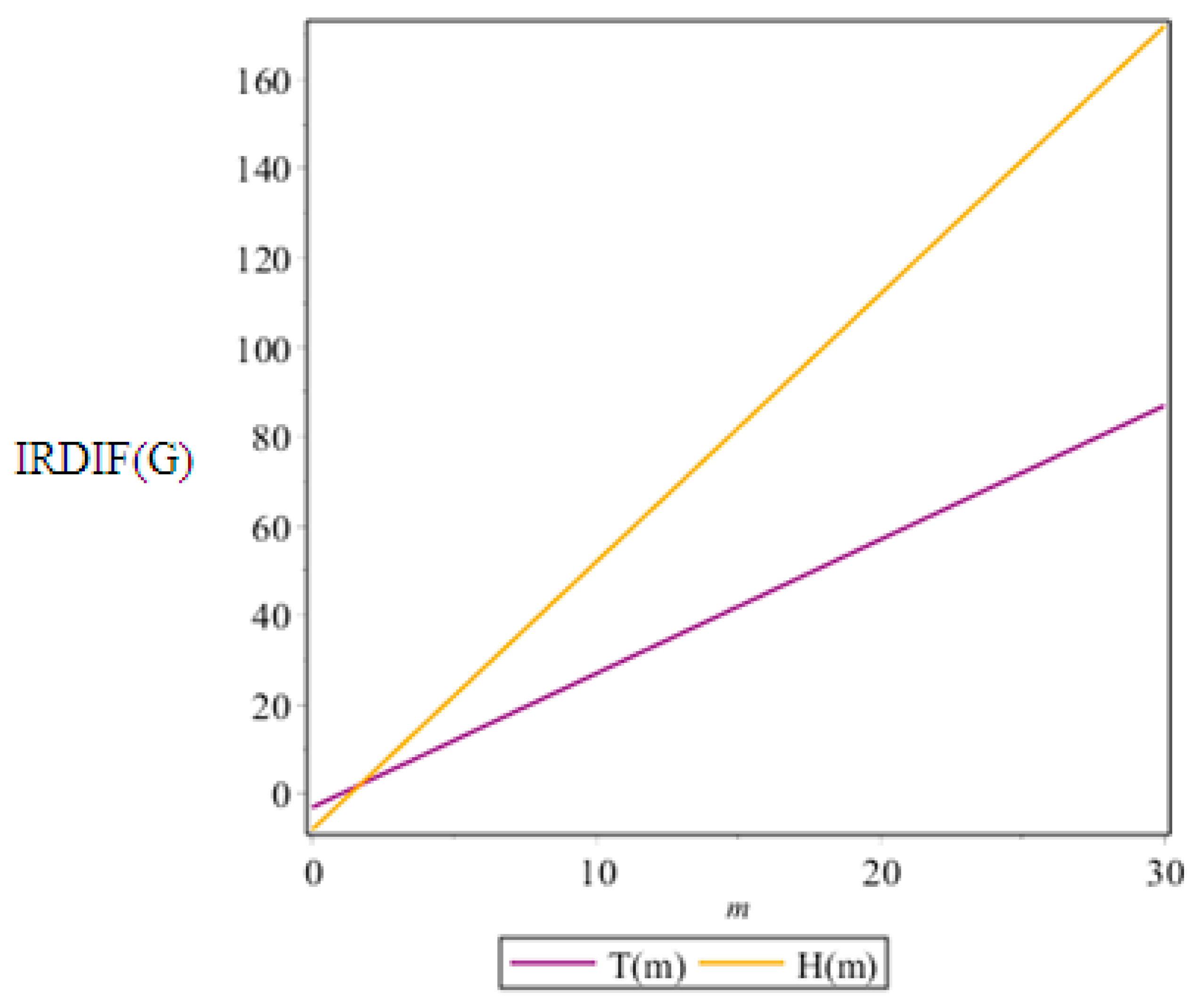
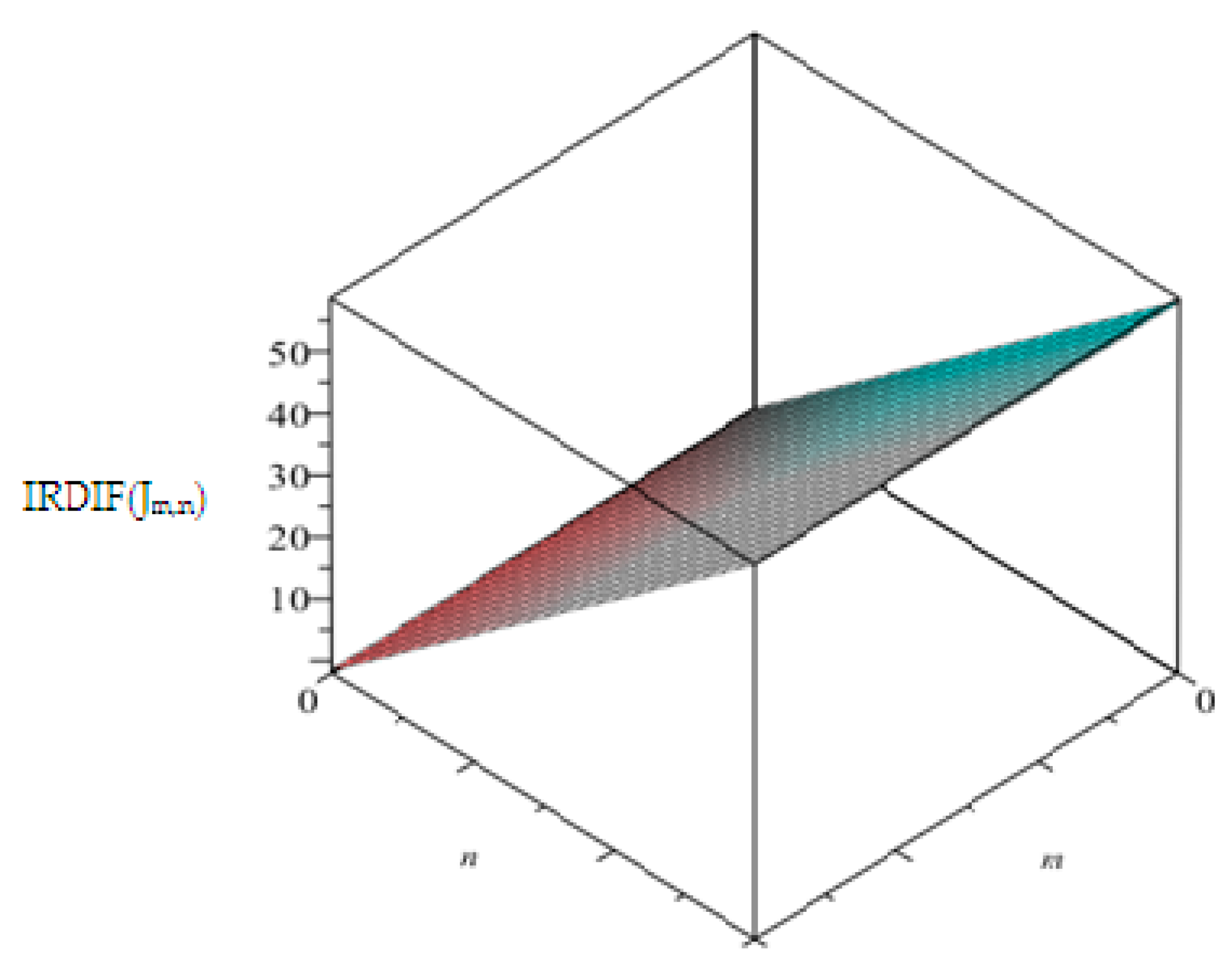
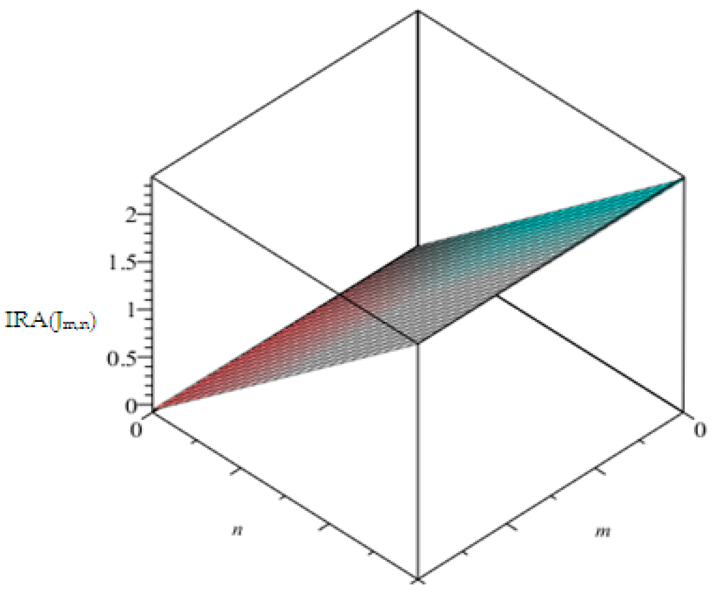
4. Graphical Analysis, Discussions, and Conclusions

In this part, we will discuss our theoretical results and conclude which of the above described benzenoid systems is more irregular than the other, with respect to a particular irregularity index. Systems $T_m$, $H_m$ depend on a single parameter m, and all closed relations of irregularity indices are linear in m, so the graphs of these indices should be straight lines, whereas $J_{m,n}$ depends on two parameters, and the obtained graph is a planar surface. We plot $T_m$, $H_m$ on a single graph and $J_{m,n}$ as a separate graph.

We see that all irregularity indices tend to increase with increases in the values of the parameters. We gave graphical behaviors of some of these indices with respect to the change in the parameter of m. In this graphical analysis, the purple color shows the graphical behavior of the triangular benzenoid system, the orange color shows the graphical behavior of the hourglass benzenoid system, and the 3D surface shows the graphical behavior of the jagged-rectangle benzenoid with respect to both variables m and n for the range of parameters m = 0…30 and n = 0…30. We give the graph of irregularity in $IRDIF\left(G\right)$ in Figure 5. Comparative behavior of $IRDIF\left(G\right)$ $for{T}_m$ and $H_m$ is elaborated in this figure.

Figure 6 is a 3D plot for $IRDIF\left(J_{m,n}\right)$. The values of this index increase with an increase in both parameter m and n.

Now we see the behavior of the irregularity index $IRA\left(G\right)$ for the range of parameters m = 0…30 and n = 0…30. In the Figure 7, we give the irregularity index $IRA\left(G\right)$ for $T_m$ and $H_m$.

Next, we give the 3D surface of the irregularity index $IRA\left(J_{m,n}\right)$ for $J_{m,n}$ in Figure 8, with respect to both parameters m and n simultaneously.

These graphs graphically depict that the values of all irregularity indices increase with an increase in the variable of the structures. Figure 5 and Figure 7 show that the molecular structure of benzenoid hourglass H(m) is highly irregular, as compared to the triangular benzenoid system.

We foresee that our results could play an important role in determining the properties of these benzenoid systems, such boiling point, heats of vaporization, enthalpy, and entropy. Similar work has been done in [29], where authors discussed some properties of alkane isomers.

References

1. Gutman, I.; Cyvin, S.V. Introduction to the Theory of Benzenoid Hydrocarbons; Springer: Berlin, Germany, 1989. [Google Scholar]
2. Rucker, G.; Rucker, C. On topological indices, boiling points, and cyclo-alkanes. J. Chem. Inf. Comput. Sci. 1999, 39, 788–802. [Google Scholar] [CrossRef]
3. Gutman, I.; Polansky, O.E. Mathematical Concepts in Organic Chemistry; Springer: New York, NY, USA, 1986. [Google Scholar]
4. Randic, M. On the characterization of molecular branching. J. Am. Chem. Soc. 1975, 97, 6609–6615. [Google Scholar] [CrossRef]
5. Wiener, H. Structural determination of paraffin boiling points. J. Am. Chem. Soc. 1947, 69, 17–20. [Google Scholar] [CrossRef] [PubMed]
6. Estrada, E. Atomic bond connectivity and the energetic of branched alkanes. Chem. Phys. Lett. 2008, 463, 422–425. [Google Scholar] [CrossRef]
7. Kier, L.; Hall, L. Molecular Connectivity in Chemistry and Drug Research; Academic Press: New York, NY, USA, 1976. [Google Scholar]
8. Kier, L.B.; Hall, L.H. Molecular Connectivity in Structure Activity Analysis; Wiley: New York, NY, USA, 1986. [Google Scholar]
9. Kwun, Y.C.; Ali, A.; Nazeer, W.; Ahmad Chaudhary, M.; Kang, S.M. M-Polynomials and Degree-Based Topological Indices of Triangular, Hourglass, and Jagged-Rectangle Benzenoid Systems. J. Chem. 2018. [Google Scholar] [CrossRef]
10. Deng, H.; Yang, J.; Xia, F. A general modeling of some vertex-degree based topological indices in benzenoid systems and phenylenes. Compt. Math. Appl. 2011, 61, 3017–3023. [Google Scholar] [CrossRef] [Green Version]
11. Zhang, H.; Zhang, F. The Clar covering polynomial of hexagonal systems. Discret. Appl. Math. 1996, 69, 147–167. [Google Scholar] [CrossRef]
12. Munir, M.; Nazeer, W.; Rafique, S.; Kang, S.M. Mpolynomial and related topological indices of Nanostar dendrimers. Symmetry 2016, 8, 97. [Google Scholar] [CrossRef]
13. Munir, M.; Nazeer, W.; Rafique, S.; Nizami, A.R.; Kang, S.M. M-polynomial and degree-based topological indices of titania nanotubes. Symmetry 2016, 8, 117. [Google Scholar] [CrossRef]
14. Munir, M.; Nazeer, W.; Rafique, S.; Kang, S.M. M-Polynomial and Degree-Based Topological Indices of Polyhex Nanotubes. Symmetry 2016, 8, 149. [Google Scholar] [CrossRef]
15. Munir, M.; Nazeer, W.; Shahzadi, S.; Kang, S.M. Some invariants of circulant graphs. Symmetry 2016, 8, 134. [Google Scholar] [CrossRef]
16. Chartrand, G.; Erdos, P.; Oellermann, O. How to define an irregular graph. Coll. Math. J. 1988, 19, 36–42. [Google Scholar] [CrossRef]
17. Majcher, Z.; Michael, J. Highly irregular graphs with extreme numbers of edges. Discr. Math. 1997, 164, 237–242. [Google Scholar] [CrossRef] [Green Version]
18. Behzad, M.; Chartrand, G. No graph is perfect. Am. Math. Mon. 1947, 74, 962–963. [Google Scholar] [CrossRef]
19. Horoldagva, B.; Buyantogtokh, L.; Dorjsembe, S.; Gutman, I. Maximum sizeof maximally irregular graphs. Match Commun. Math. Comput. Chem. 2016, 76, 81–98. [Google Scholar]
20. Liu, F.; Zhang, Z.; Meng, J. The size of maximally irregular graphs and maximally irregular triangle–free graphs. Graphs Comb. 2014, 30, 699–705. [Google Scholar] [CrossRef]
21. Collatz, L.; Sinogowitz, U. Spektren endlicher Graphen. Abh. Math. Sem. Univ. Hamburg 1957, 21, 63–77. [Google Scholar]
22. Bell, F.K. A note on the irregularity of graphs. Linear Algebra Appl. 1992, 161, 45–54. [Google Scholar] [CrossRef] [Green Version]
23. Albertson, M. The irregularity of a graph. Ars Comb. 1997, 46, 219–225. [Google Scholar]
24. Vukičević, D.; Graovac, A. Valence connectivities versus Randić, Zagreb and modified Zagreb index: A linear algorithm to check discriminative properties of indices in acyclic molecular graphs. Croat. Chem. Acta 2004, 77, 501–508. [Google Scholar]
25. Abdo, H.; Brandt, S.; Dimitrov, D. The total irregularity of a graph. Discr. Math. Theor. Comput. Sci. 2014, 16, 201–206. [Google Scholar]
26. Abdo, H.; Dimitrov, D. The total irregularity of graphs under graph operations. Miskolc Math. Notes 2014, 15, 3–17. [Google Scholar] [CrossRef]
27. Abdo, H.; Dimitrov, D. The irregularity of graphs under graph operations. Discuss. Math. Graph. Theory 2014, 34, 263–278. [Google Scholar] [CrossRef]
28. Gutman, I. Topological Indices and Irregularity Measures. J. Bull. 2018, 8, 469–475. [Google Scholar]
29. Reti, T.; Sharfdini, R.; Dregelyi-Kiss, A.; Hagobin, H. Graph irregularity indices used as molecular discriptors in QSPR studies. MATCH Commun. Math. Comput. Chem. 2018, 79, 509–524. [Google Scholar]
30. Hu, Y.; Li, X.; Shi, Y.; Xu, T.; Gutman, I. On molecular graphs with smallest and greatest zeroth-Corder general randic index. MATCH Commun. Math. Comput. Chem. 2005, 54, 425–434. [Google Scholar]
31. Caporossi, G.; Gutman, I.; Hansen, P.; Pavlovic, L. Graphs with maximum connectivity index. Comput. Biol. Chem. 2003, 27, 85–90. [Google Scholar] [CrossRef]
32. Li, X.; Gutman, I. Mathematical aspects of Randic, Type molecular structure descriptors. In Mathematical Chemistry Monographs; University of Kragujevac and Faculty of Science Kragujevac: Kragujevac, Serbia, 2006. [Google Scholar]
33. Das, K.; Gutman, I. Some properties of the second Zagreb Index. MATCH Commun. Math. Comput. Chem. 2004, 52, 103–112. [Google Scholar]
34. Trinajstic, N.; Nikolic, S.; Milicevic, A.; Gutman, I. About the Zagreb Indices. Kemija u industriji: Časopis kemičara i kemijskih inženjera Hrvatske 2010, 59, 577–589. [Google Scholar]
35. Milicevic, A.; Nikolic, S.; Trinajstic, N. On reformulated Zagreb indices. Mol. Divers. 2004, 8, 393–399. [Google Scholar] [CrossRef]
36. Gupta, C.K.; Lokesha, V.; Shwetha, S.B.; Ranjini, P.S. On the symmetric division DEG index of graph. Southeast Asian Bull. Math. 2016, 40, 59–80. [Google Scholar]
37. Balaban, A.T. Highly discriminating distance based numerical descriptor. Chem. Phys. Lett. 1982, 89, 399–404. [Google Scholar] [CrossRef]
38. Furtula, B.; Graovac, A.; Vukičević, D. Augmented Zagreb index. J. Math. Chem. 2010, 48, 370–380. [Google Scholar] [CrossRef]
39. Das, K.C. Atom–bond connectivity index of graphs. Discr. Appl. Math. 2010, 158, 1181–1188. [Google Scholar] [CrossRef]
40. Estrada, E.; Torres, L.; Rodríguez, L.; Gutman, I. An atom–bond connectivity index: Modeling the enthalpy of formation of alkanes. Indian. J. Chem. 1998, 37, 849–855. [Google Scholar]
41. Zahid, I.; Aslam, A.; Ishaq, M.; Aamir, M. Characteristic study of irregularity measures of some Nanotubes. Can. J. Phys. 2019. [Google Scholar] [CrossRef]
42. Gao, W.; Aamir, M.; Iqbal, Z.; Ishaq, M.; Aslam, A. On Irregularity Measures of Some Dendrimers Structures. Mathematics 2019, 7, 271. [Google Scholar] [CrossRef]
43. Gao, W.; Abdo, H.; Dimitrov, D. On the irregularity of some molecular structures. Can. J. Chem. 2017, 95, 174–183. [Google Scholar] [CrossRef] [Green Version]
Figure 1. Non-isomorphic benzenoid structures for h = 2, 3, 4.
Processes 07 00413 g001
Figure 2. Triangular benzenoid system Tm.
Processes 07 00413 g002
Figure 3. Hourglass benzenoid system H m .
Processes 07 00413 g003
Figure 4. Jagged-rectangle benzenoid system J m , n .
Processes 07 00413 g004
Figure 5. G r a p h i c a l   c o m p a r i s i o n   o f   I R D I F   f o r   T m   a n d   H m against parameter m.
Processes 07 00413 g005
Figure 6. 3 D   G r a p h i c a l   b e h a v i o r of I R D I F   f o r   J m , n against both parameters m and n.
Processes 07 00413 g006
Figure 7. G r a p h i c a l   c o m p a r i s i o n   o f   I R A   f o r   T m   a n d   H m against parameter m.
Processes 07 00413 g007
Figure 8. 3 D   G r a p h i c a l   b e h a v i o r of I R A   f o r   J m , n against both parameters m and n.
Processes 07 00413 g008