Gaussian Process-Based Hybrid Model for Predicting Oxygen Consumption in the Converter Steelmaking Process


Abstract
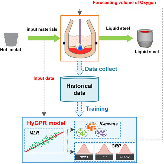
1. Introduction
2. Methodology
- (1)
- The amount of input materials, such as the carbon, silicon, manganese, phosphorus, sulfur content of hot metal.
- (2)
- The control parameters of blowing, e.g., lance position, and blowing pattern.
- (3)
- The final smelting targets, e.g., oxygen consumption highly depends on the carbon target.
- (4)
- The equipment conditions, e.g., converter lining and internal converter geometry.
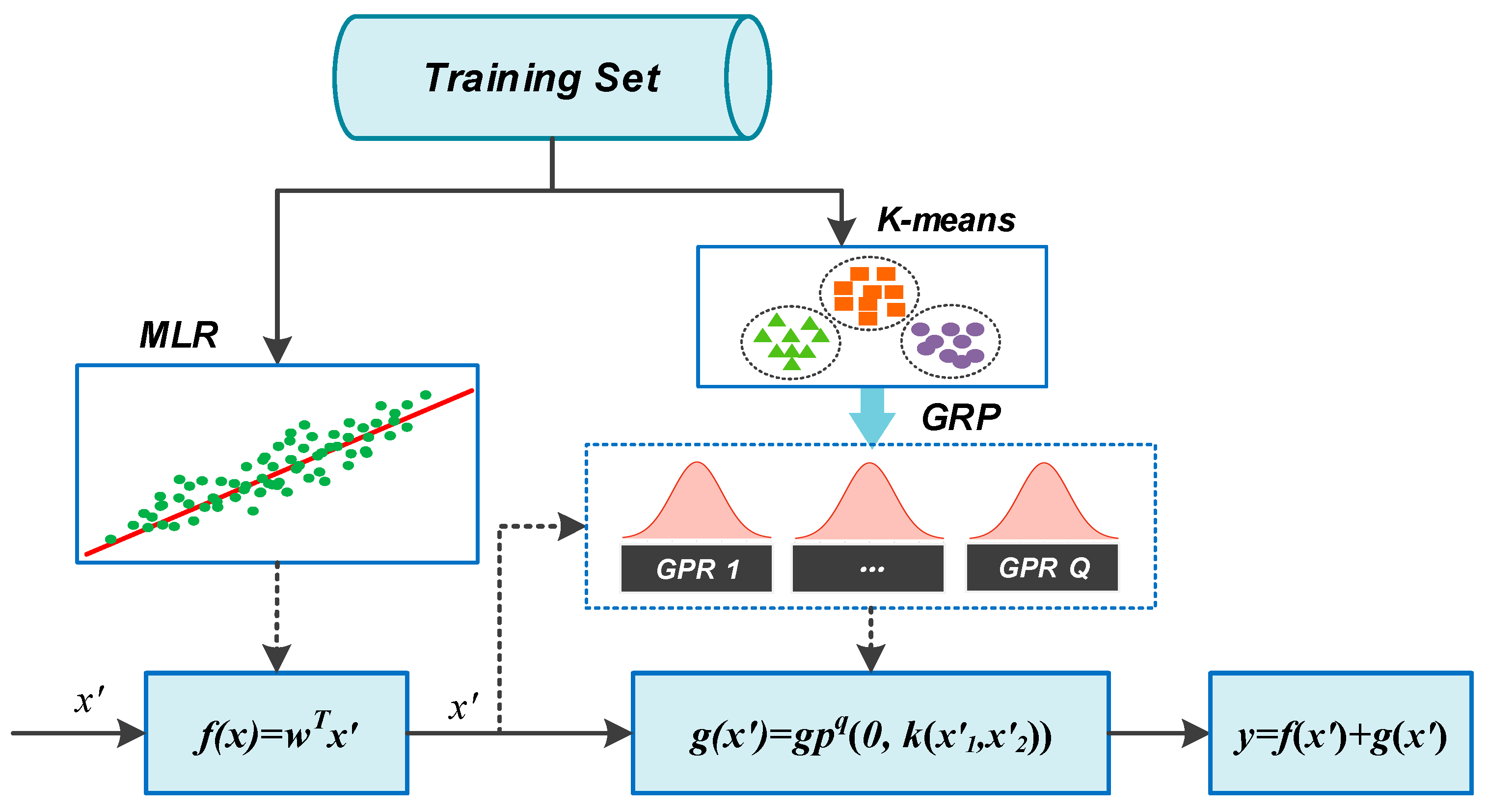
2.1. Reaction-Based Linear Model
2.2. Gaussian Process Regression with Noise
2.3. HyGPR with K-Means Clustering
3. Experiments and Discussion
3.1. Data Set
- (1)
- The weight of hot metal (Fe).
- (2)
- The weight of impurity elements, e.g., carbon (C), silicon (Si), manganese (Mn), sulphur (S) and phosphorus (S) which are the products of the weights of hot metal and the element percentages.
- (3)
- Five additional materials (AM) for steelmaking, of which the real compositions are secreted.
3.2. Evaluation Metrics
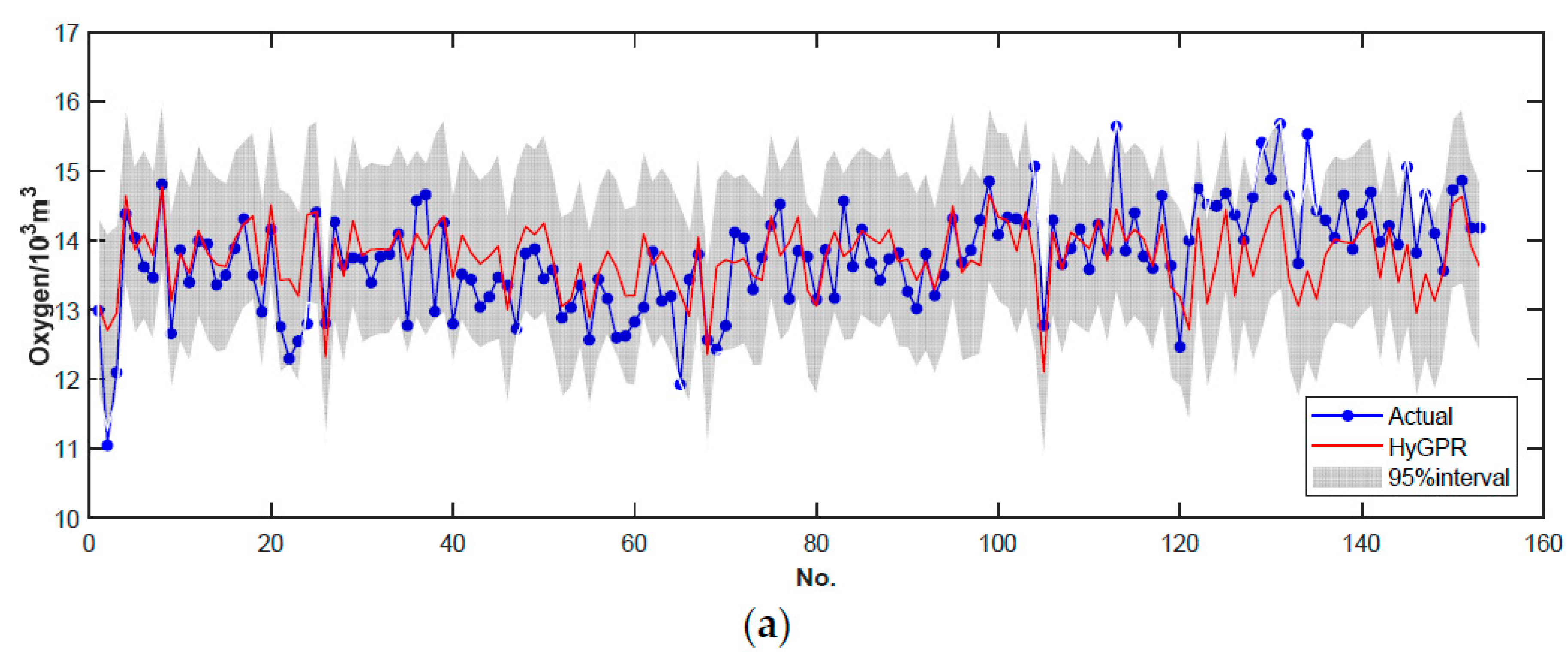
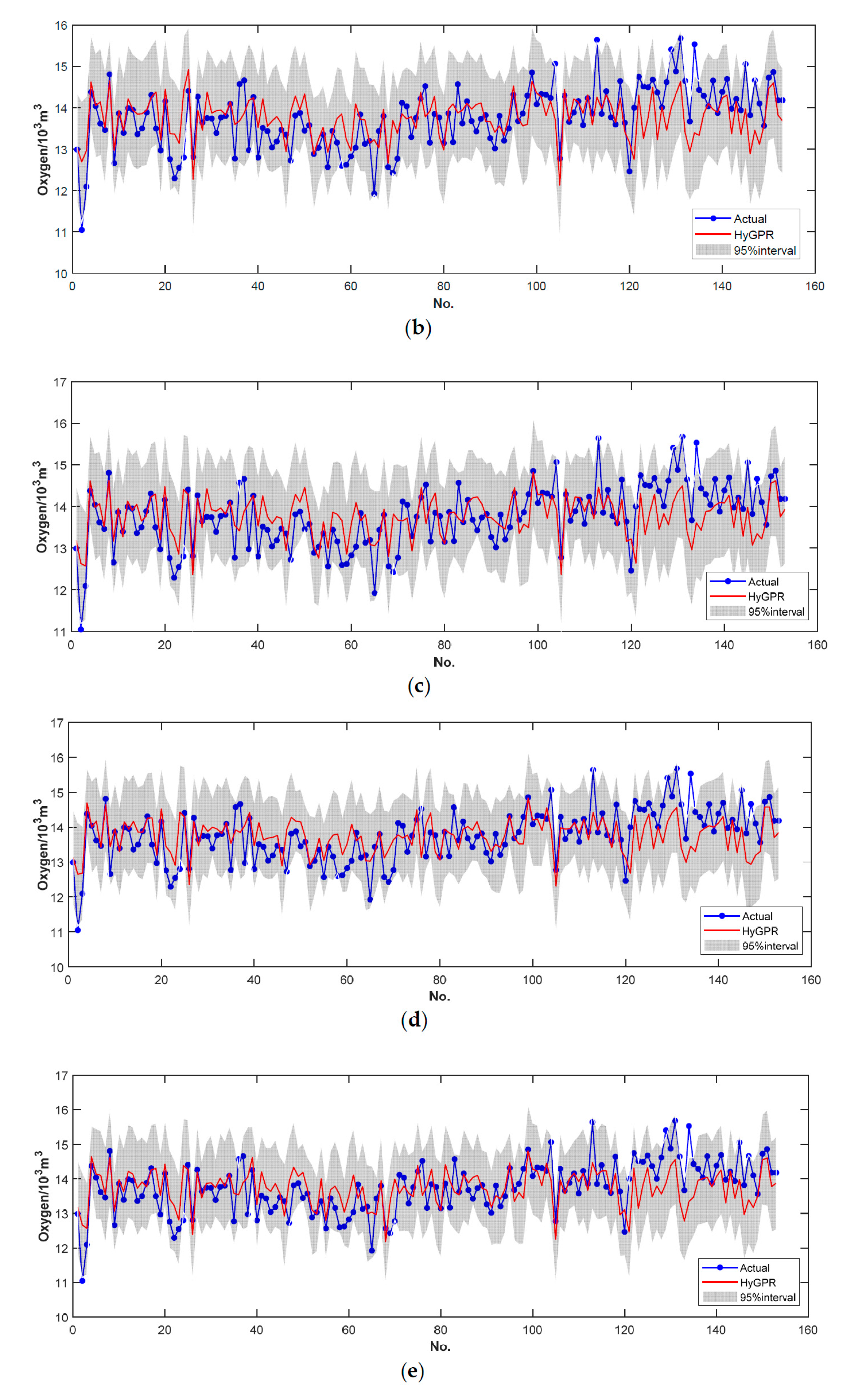
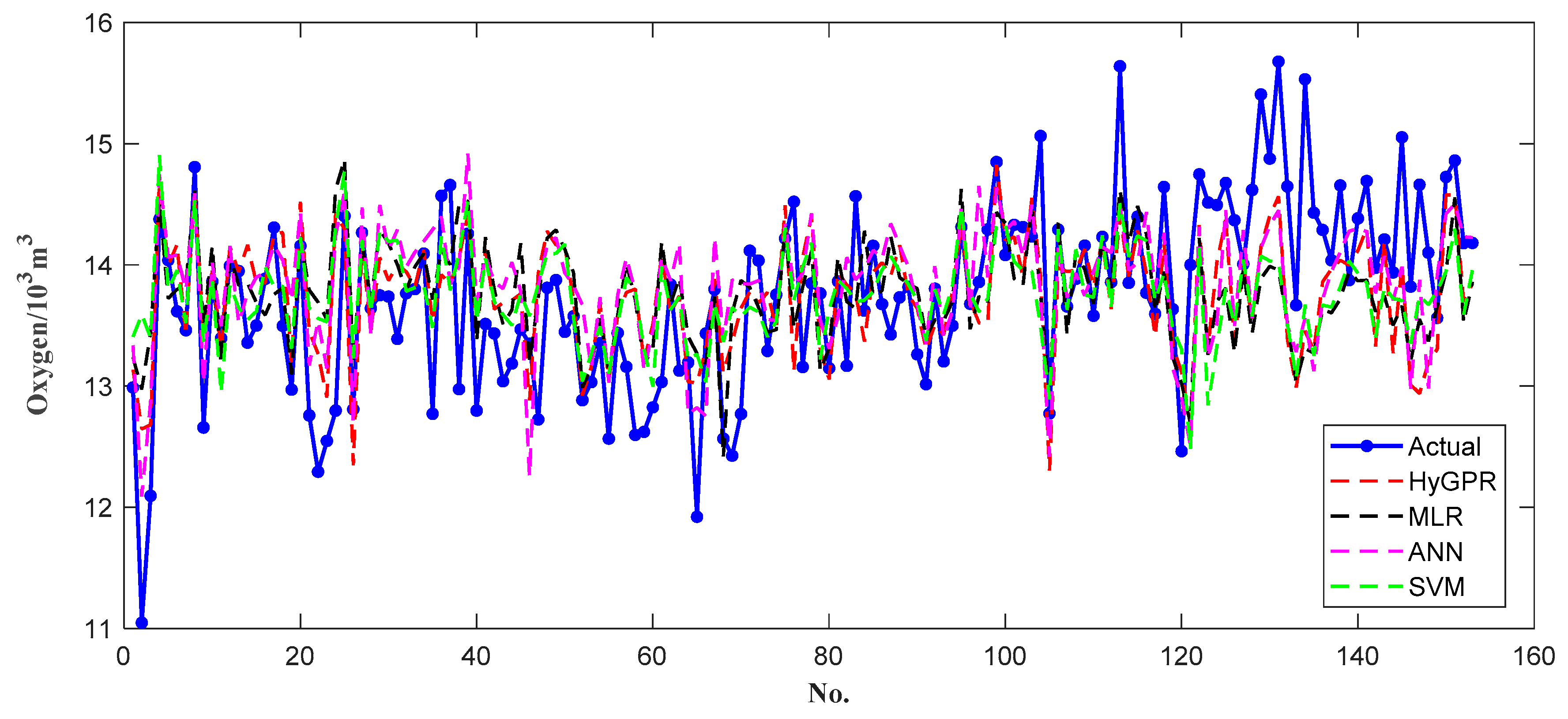
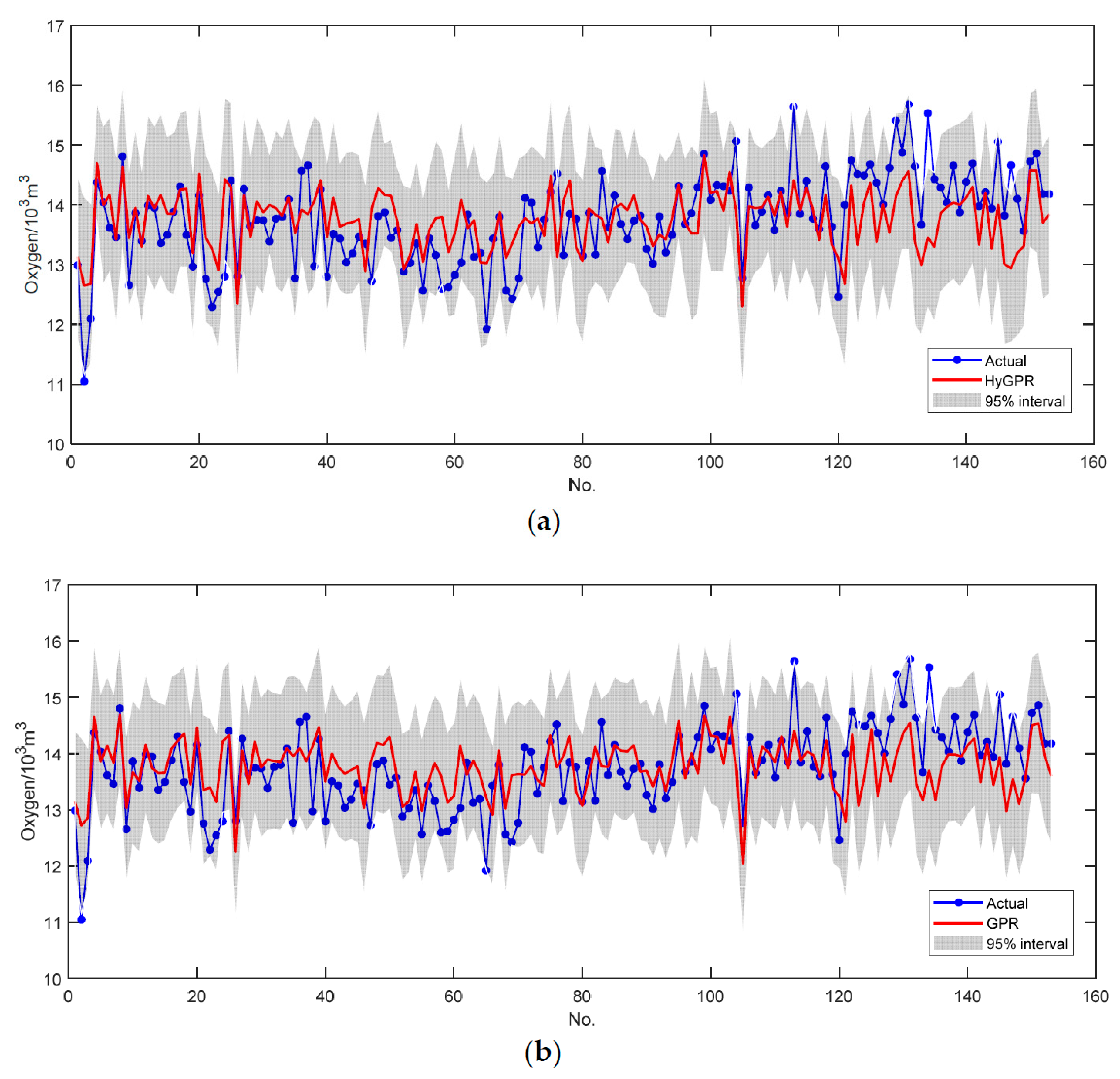
3.3. Results and Analysis
4. Conclusions
- (1).
- The online prediction model involving dynamic operating parameters, such as the position of oxygen lance, the pressure of oxygen blowing and the duration of oxygen blowing.
- (2).
- The prediction model to forecast slopping events, which is very important to reduce production costs and environmental impacts.
- (3).
- In this study, we assume that the noise of the steelmaking process is a Gaussian distribution. However, when it comes to the small-sample and high-dimensional data set, the assumption is incorrect. So it needs to develop a non-Gaussian prediction model applied in other environments.
Author Contributions
Funding
Acknowledgments
Conflicts of Interest
References
- Han, Z.; Zhao, J.; Wang, W.; Liu, Y. A two-stage method for predicting and scheduling energy in an oxygen/nitrogen system of the steel industry. Control. Eng. Pract. 2016, 52, 35–45. [Google Scholar] [CrossRef]
- Fan, J. Research on Production Scheduling and Charge Energy Consumption Prediction of Converter in Steelmaking Works. Master’s Thesis, Chongqing University, Chongqing, China, May 2018. (In Chinese). [Google Scholar]
- Han, Z.; Zhao, J.; Wang, W. An optimized oxygen system scheduling with electricity cost consideration in steel industry. IEEE/CAA J. Autom. Sin. 2017, 4, 216–222. [Google Scholar] [CrossRef]
- Alam, M.; Naser, J.; Brooks, G. Computational fluid dynamics simulation of supersonic oxygen jet behavior at steelmaking temperature. Metall. Mater. Trans. B 2010, 41, 636–645. [Google Scholar] [CrossRef]
- Ghosh, A. Secondary Steelmaking: Principles and Applications; CRC Press: Boca Raton, FL, USA, 2000. [Google Scholar]
- Reis, M.; Gins, G. Industrial process monitoring in the big data/industry 4.0 era: From detection, to diagnosis, to prognosis. Processes 2017, 5, 35. [Google Scholar] [CrossRef]
- Kadlec, P.; Gabrys, B.; Strandt, S. Data-driven soft sensors in the process industry. Comput. Chem. Eng. 2009, 33, 795–814. [Google Scholar] [CrossRef]
- Kadlec, P.; Grbić, R.; Gabrys, B. Review of adaptation mechanisms for data-driven soft sensors. Comput. Chem. Eng. 2011, 35, 1–24. [Google Scholar] [CrossRef]
- Duan, Y.; Liu, M.; Dong, M.; Wu, C. A two-stage clustered multi-task learning method for operational optimization in chemical mechanical polishing. J. Process Control 2015, 35, 169–177. [Google Scholar] [CrossRef]
- Li, D. Perspective for smart factory in petrochemical industry. Comput. Chem. Eng. 2016, 91, 136–148. [Google Scholar] [CrossRef]
- Liukkonen, M.; Hälikkä, E.; Hiltunen, T.; Hiltunen, Y. Dynamic soft sensors for NOx emissions in a circulating fluidized bed boiler. Appl. Energy 2012, 97, 483–490. [Google Scholar] [CrossRef]
- Cox, I.J.; Lewis, R.W.; Ransing, R.S.; Laszczewski, H.; Berni, G. Application of neural computing in basic oxygen steelmaking. J. Mater. Process. Technol. 2002, 120, 310–315. [Google Scholar] [CrossRef]
- Zhou, X.; Yang, C.; Gui, W. Modeling and control of nonferrous metallurgical processes on the perspective of global optimization. Control. Theory Appl. 2015, 32, 1158–1169. [Google Scholar]
- Saxén, H.; Gao, C.; Gao, Z. Data-driven time discrete models for dynamic prediction of the hot metal silicon content in the blast furnace—A review. IEEE Trans. Ind. Inform. 2013, 9, 2213–2225. [Google Scholar] [CrossRef]
- Liu, C.; Tang, L.; Liu, J.; Tang, Z. A dynamic analytics method based on multistage modeling for a BOF steelmaking process. IEEE Trans. Autom. Sci. Eng. 2018, 1–13. [Google Scholar] [CrossRef]
- Tian, H.X.; Mao, Z.Z. An ensemble ELM based on modified AdaBoost. RT algorithm for predicting the temperature of molten steel in ladle furnace. IEEE Trans. Autom. Sci. Eng. 2010, 7, 73–80. [Google Scholar] [CrossRef]
- Han, M.; Liu, C. Endpoint prediction model for basic oxygen furnace steel-making based on membrane algorithm evolving extreme learning machine. Appl. Soft Comput. 2014, 19, 430–437. [Google Scholar] [CrossRef]
- Laha, D.; Ren, Y.; Suganthan, P.N. Modeling of steelmaking process with effective machine learning techniques. Expert Syst. Appl. 2015, 42, 4687–4696. [Google Scholar] [CrossRef]
- Yang, J.; Chai, T.; Luo, C.; Yu, W. Intelligent Demand Forecasting of Smelting Process Using Data-Driven and Mechanism Model. IEEE Trans. Ind. Electron. 2018. [Google Scholar] [CrossRef]
- Chen, J.; Chandrashekhara, K.; Mahimkar, C.; Lekakh, S.N.; Richards, V.L. Void closure prediction in cold rolling using finite element analysis and neural network. J. Mater. Process. Technol. 2011, 211, 245–255. [Google Scholar] [CrossRef]
- Lei, Z.; Su, W. Mold Level Predict of Continuous Casting Using Hybrid EMD-SVR-GA Algorithm. Processes 2019, 7, 177. [Google Scholar] [CrossRef]
- Friedman, J.; Hastie, T.; Tibshirani, R. The Elements of Statistical Learning; Springer: Berlin, Germany, 2001. [Google Scholar]
- Williams, C.K.; Rasmussen, C.E. Gaussian Processes for Machine Learning; MIT Press: Cambridge, MA, USA, 2006. [Google Scholar]
- Schulz, E.; Speekenbrink, M.; Krause, A. A tutorial on Gaussian process regression: Modelling, exploring, and exploiting functions. J. Math. Psychol. 2018, 85, 1–16. [Google Scholar] [CrossRef]
- Shawe-Taylor, J.; Cristianini, N. Kernel Methods for Pattern Analysis; Cambridge University Press: Cambridge, UK, 2004. [Google Scholar]
- Rasmussen, C.E.; Nickisch, H. Gaussian processes for machine learning (GPML) toolbox. J. Mach. Learn. Res. 2010, 11, 3011–3015. [Google Scholar]
- Laha, D. ANN modeling of a steelmaking process. In Proceedings of the International Conference on Swarm, Evolutionary, and Memetic Computing, Chennai, India, 19–21 December 2013; Springer: Cham, Switzerland, 2013. [Google Scholar]
- Smola, A.J.; Schölkopf, B. A tutorial on support vector regression. Stat. Comput. 2004, 14, 199–222. [Google Scholar] [CrossRef]


| Parameters | Mean. | Std. | Minimum | Maximum |
|---|---|---|---|---|
| Fe (t) | 276.8450 | 252.7000 | 289.8000 | 21.6711 |
| C (t) | 12.1259 | 0.5061 | 10.3288 | 14.0078 |
| Si (t) | 0.9477 | 0.4456 | 0.0318 | 2.332 |
| Mn (t) | 0.4332 | 0.2047 | 0.1252 | 2.2066 |
| P (t) | 0.2431 | 0.0221 | 0.1736 | 0.4119 |
| S (t) | 0.0023 | 0.0022 | 0 | 0.0343 |
| AM1 (t) | 1.7980 | 1.4659 | 0 | 9.908 |
| AM2 (t) | 1.7487 | 1.6683 | 0 | 8.172 |
| AM3 (t) | 14.1139 | 2.5374 | 5.9610 | 28.937 |
| AM4 (t) | 4.1623 | 1.3636 | 0 | 9.66 |
| AM5 (t) | 0.7833 | 1.6976 | 0 | 11.994 |
| O2 (103m3) | 13.7823 | 0.8079 | 11.0480 | 15.913 |
| Cluster Count | RMSE (103m3) | MAE (103m3) | MAPE (%) | CPU Time (S) |
|---|---|---|---|---|
| Q = 1 | 0.64 | 0.49 | 3.56 | 62.47 |
| Q = 2 | 0.64 | 0.48 | 3.51 | 27.62 |
| Q = 3 | 0.63 | 0.49 | 3.55 | 19.82 |
| Q = 4 | 0.63 | 0.48 | 3.52 | 13.32 |
| Q = 5 | 0.64 | 0.53 | 3.90 | 15.49 |
| Model | RMSE (103m3) | MAE (103m3) | MAPE (%) |
|---|---|---|---|
| MLR | 0.70 | 0.54 | 3.95 |
| SVM | 0.69 | 0.53 | 3.92 |
| ANN | 0.68 | 0.52 | 3.84 |
| HyGPR | 0.63 | 0.48 | 3.52 |
| Model | RMSE (103m3) | MAE (103m3) | MAPE (%) | HRI (%) | CPU (S) |
|---|---|---|---|---|---|
| GPR | 0.63 | 0.49 | 3.59 | 92.42% | 75.74 |
| HyGPR | 0.63 | 0.48 | 3.52 | 96.08% | 14.14 |
© 2019 by the authors. Licensee MDPI, Basel, Switzerland. This article is an open access article distributed under the terms and conditions of the Creative Commons Attribution (CC BY) license (http://creativecommons.org/licenses/by/4.0/).
Share and Cite
Jiang, S.-L.; Shen, X.; Zheng, Z. Gaussian Process-Based Hybrid Model for Predicting Oxygen Consumption in the Converter Steelmaking Process. Processes 2019, 7, 352. https://doi.org/10.3390/pr7060352
Jiang S-L, Shen X, Zheng Z. Gaussian Process-Based Hybrid Model for Predicting Oxygen Consumption in the Converter Steelmaking Process. Processes. 2019; 7(6):352. https://doi.org/10.3390/pr7060352
Chicago/Turabian StyleJiang, Sheng-Long, Xinyue Shen, and Zhong Zheng. 2019. "Gaussian Process-Based Hybrid Model for Predicting Oxygen Consumption in the Converter Steelmaking Process" Processes 7, no. 6: 352. https://doi.org/10.3390/pr7060352
APA StyleJiang, S.-L., Shen, X., & Zheng, Z. (2019). Gaussian Process-Based Hybrid Model for Predicting Oxygen Consumption in the Converter Steelmaking Process. Processes, 7(6), 352. https://doi.org/10.3390/pr7060352