Designing, Developing and Validating a Forecasting Method for the Month Ahead Hourly Electricity Consumption in the Case of Medium Industrial Consumers

Abstract

An accurate forecast of the electricity consumption is particularly important to both consumers and system operators. The purpose of this study is to develop a forecasting method that provides such an accurate forecast of the month-ahead hourly electricity consumption in the case of medium industrial consumers, therefore assuring an intelligent energy management and an efficient economic scheduling of their resources, having the possibility to negotiate in advance appropriate billing tariffs relying on accurate hourly forecasts, in the same time facilitating an optimal energy management for the dispatch operator. The forecasting method consists of developing first non-linear autoregressive, with exogenous inputs (NARX) artificial neural networks (ANNs) in order to forecast an initial daily electricity consumption, a forecast that is being further processed with custom developed long short-term memory (LSTM) neural networks with exogenous variables support in order to refine the daily forecast as to achieve an accurate hourly forecasted consumed electricity for the whole month-ahead. The obtained experimental results (highlighted also through a very good value of 0.0244 for the root mean square error performance metric, obtained when forecasting the month-ahead hourly electricity consumption and comparing it with the real consumption), the validation of the developed forecasting method, the comparison of the method with other forecasting approaches from the scientific literature substantiate the fact that the proposed approach manages to fill a gap in the current body of knowledge consisting of the need of a high-accuracy forecasting method for the month-ahead hourly electricity consumption in the case of medium industrial consumers. The developed forecasting method targets medium industrial consumers, but, due to its accuracy, it can also be a useful tool for promoting innovative business models with regard to industrial consumers willing to produce a part of their own electricity using renewable energy resources, benefiting from reduced production costs and reliable electricity prices.

1. Introduction

1.1. Motivation

Over the course of history, the evolution of industry has been tightly linked and strongly influenced by the industrial energy consumption. Worldwide today, more than ever, the whole industry sector, no matter what its targeted final products are, ranging from developing high-technology equipment up to bakery products, is dependent on energy in each of its production stages and steps. Nowadays, due to the continuous and exponential evolution of the industry sector, in order for it to progress, the electricity consumption faces increased requirements from the quantity and quality points of view.

According to a recent report [1], the industrial activity consumes approximately half of the world’s energy, the electricity demand in this sector having soared worldwide from 22 quadrillion British thermal units (BTUs) in 2000, to 36 quadrillion BTUs in 2016 and up to a projected 39 quadrillion BTUs for the year 2020. Taking into account these statistics, one can remark that increasing the energy efficiency in the industrial sector has considerable effects in saving fuels and reducing pollutants.

Most of the economies based mainly on light industry, digital technologies or on services are relying more and more on electricity as an energy source. Worldwide, the electricity sector represents almost 20% from the global final energy consumption and the percentage is in a continuous growing [2]. According to [3,4], the worldwide electricity consumption has increased from 14,280 billion kW h in 2005, to 21,360 billion kW h in 2018.

The worldwide electricity consumption by sectors is strongly influenced by the global economic structure, which nowadays is undergoing a restructuring process and also by the national economic development situation of each country. In a series of economically-developed countries (United States of America, Japan, United Kingdom), the electricity consumptions’ structure analysis highlights an equilibrium between a part of the economy’s sectors, meaning that industries, commercial services and residential sectors exhibit comparable shares, as opposed to the transportation and agriculture sectors that represent low percentages from the total electricity consumption. Contrasting this situation, the industrial electricity consumption is higher than 73% in China, 57% in Russia, 51% in South Korea, while in Germany and Italy being higher than 44% of the total electricity consumption [2].

In Romania, according to the latest report of the National Energy Regulatory Authority (issued in July 2018, based on the statistical information retrieved for the year 2017), at the national level, the yearly final electricity consumption in 2017 was about 48.4 terawatt hours (TW h), being 3% higher when compared to the previous year. The largest amount from this total consumption comes from the non-household final consumers segment, the consumption being 35.8 TW h, which represents a percentage of 74%, while the households’ segment consumption of 12.6 TW h represents the remaining of the 26% from the total annual consumption for the year 2017 [5].

In this context, a factor of paramount importance in assuring the world’s necessary resources and a sustainable consumption of energy is to streamline the industrial production process and, equally important, to achieve a proper management of the electricity consumption. In this purpose, accurate forecasts of the consumed electricity are particularly important to industrial consumers as to devise cost-effective production plans in terms of electricity consumption while maximizing the productivity. Therefore, there is an increasing interest in the scientific literature regarding the development of accurate electricity consumption forecasting methods that are able to provide valuable decision support information to industrial consumers with regard to their energetic needs.

In the following, in order to highlight the current state of knowledge and to contextualize the research within this paper, a literature review related to the approached subject is performed. The main purpose of this subsection is to identify and state a clear gap in the current state of knowledge that is being addressed by the developed forecasting method.

1.2. Literature Review

In the scientific article [6], Wang et al. proposed a “grey prediction model improved by means of convolution integral (GMC(1,n))” along with a nonlinear optimization model developed in order to find the optimal parameters as to minimize the error. The authors applied their devised forecasting method to the industrial energy consumption of China and concluded that their proposed approach offers better results in terms of forecasting accuracy when compared to GMC(1,n), “seasonal autoregressive moving average (SARMA)” and grey model (GM(1,1)). In the final concluding remarks, the authors note that after having applied the model, a very high level of industrial energy consumption is forecasted to take place in the following years and encourage future works to focus on the related environmental impact of the industrial sector’s energy consumption.

Within the scientific paper [7], Bracale et al. aim to predict the short-term industrial reactive power based on support vector and multiple linear regression techniques. The authors remark that industrial load forecasting poses many challenges as it depends upon a wide variety of factors like work schedule and the particularities of each specific industrial process. The data were collected from a factory situated in Italy, being recorded at 15 min intervals that were averaged as to obtain an hourly consumption dataset. After having performed the experimental tests, the authors conclude that their proposed approach offers an improved forecasting accuracy when compared to the “seasonal naïve (SN)”, “persistence model (PM)”, “seasonal auto regressive integrated moving average (SARIMA)” and the forecasts of “active power and typical averaged power factors (AVEPF)” reference benchmark models. As a future work, the authors state that they intend to improve the prediction accuracy by devising hybrid approaches.

Berk et al. propose in [8] an inhomogeneous Markov switching approach in order to forecast the electricity loads of certain industrial companies, taking into account the specific load case of this type of consumers, for which the production regime alternates with the standby one, according to the work shifts scheduling. This alternance is described using a hidden Markov chain, along with transition probabilities that vary over time, depending on a series of calendar and time variables. The electricity load is modeled using two different approaches for the two different specific regimes, namely during the production, an autoregressive moving-average model is used, while for the standby time the authors employ a model based on the white noise process. After analyzing the performance of the developed method in providing a probabilistic forecasting, the authors remark that their model outperforms many usual additive time series models.

Within the scientific article [9], Oliveira et al. propose a combined electricity forecasting method for the mid-long term by making use of “bootstrap aggregation (bagging)”, exponential smoothing techniques like the “Holt–Winters additive model”, the “Holt–Winters multiplicative model”, “state space based (exponential smoothing) formulations” along with SARIMA models. In the final processing step, the authors aggregate the predictions obtained for every bootstrapped time series using the simple mean and the simple median methods as to obtain the final result. The authors forecast the electricity consumption for several countries for a 24-months ahead period and conclude that there are potential gains in terms of forecasting accuracy that can be obtained by making use of bagged methods. In their future work, the authors intend to study in detail the possibility of applying their devised approach for predicting the electricity consumption at the level of industrial, commercial, residential and of other types of electricity consumers.

Wang et al. propose in [10] an ensemble technique based on neural networks in order to achieve an accurate forecast of the month-ahead industrial electricity consumption. The proposed approach consists of a sparse “adaptive boosting (AdaBoost)” used as an ensemble framework, an “echo state network (ESN)” along with a “fruit fly optimization algorithm (FOA)” useful for choosing the input variables based on the effects of their time lag. The authors have applied their proposed method in predicting the month-ahead electricity consumption for two industrial case studies, namely the Zhejiang and Hubei provinces from China. After having performed the experimental tests, the authors have compared the obtained results with the ones provided by other methods like “bootstrap aggregation”, “AdaBoost”, “AdaBoost with early stopping”, “model average”, “model selection” and with a single “echo state network”, therefore concluding that their proposed approach offers a higher degree of efficiency and has the advantage of reducing significantly the processing time. In the concluding remarks, the authors mention that they intend to make a more in-depth study of the two case studies when sufficient reliable data can be collected using digital side management technologies that are emerging in China. In addition, the authors intend to make use of other algorithms like the “harmony search (HS)” to improve the performance of their forecasting method further.

In the scientific article [11], Silva et al. propose a forecasting method of the long-term electricity consumption of the Brazilian pulp and paper industrial sector, using the bottom-up approach combined with the linear hierarchical models, taking into account several scenarios as to attain energy efficiency. The authors made use of the “Bayesian inference (BI)” in order to estimate the model’s parameters, therefore being able to generate sample values corresponding to every important parameter and obtain the parameters’ posterior probability distributions. For every parameter, the authors employ the “Monte Carlo Markov chain (MCMC)” method, namely the Gibbs sampling technique for obtaining the samples. The authors state that the obtained results confirm the fact that the model is able to provide an accurate forecast close to the real electricity consumption.

Hu et al. aim to achieve in [12] a prediction method for the short-term electricity consumption in the industrial papermaking process, having as a main motivation the fact that the industrial processes consume huge amounts of electricity during their production phases. The authors’ proposed method is a hybrid one, being based on “genetic algorithm (GA)”, “particle swarm optimization (PSO)” and “back propagation neural networks (BPNN)”. During the experimental tests, the authors have used real production data from two industrial consumers from the paper making business, the data of the first experimental test having been obtained from a papermill located in the Guangdong province, China, while the data for the second test having been obtained from a papermill situated in the Hubei province, China. In order to assess the performance of their proposed approach, the authors have used as performance metrics the “mean absolute percentage error (MAPE)” along with the “relative error (RE)” and have also computed the performance metrics and compared their proposed approach with the BPNN enriched with the GA, and also with the BPNN enriched with PSO, concluding that their proposed approach offers a higher level of performance and can be applied successfully in the papermaking industry fabrication process.

In the scientific paper [13], Yao et al. study the industrial electricity consumption from the perspective of industrial causality. In terms of the methods, the authors apply “Granger causality” and “partial Grainger causality” networks using electricity consumption data regarding the industries of Guangdong, Guangxi, Guizhou, Yunnan and Hunan provinces, along with the industries from South China. Afterwards, the authors have applied “bootstrap analysis” to validate the correctness of the results that confirm that the Guangdong and Guangxi provinces, along with South China, have a more solid industrial structure when compared to the other provinces. The authors state that their obtained results offer fresh perspectives from the industrial cooperation point of view, therefore being useful in predicting the industrial evolution trend and in analyzing industrial chains from an economic perspective. It is interesting to note that all the provided information the authors were able to obtain came from analyzing data regarding electricity consumption of the industrial sector.

In the research paper [14], Ding et al. design a modified grey model in view of forecasting the total and industrial electricity consumption in China for the periods of 2012–2014 (for benchmarking purposes) and 2015–2020. As the conditions of the initial grey model had several drawbacks in terms of structure and adaptability, the authors proposed initial conditions with adjustable weighted coefficients. The generating parameters were determined by applying a “PSO” algorithm to several features of the input data. A “rolling mechanism” consisting in using the latest obtained information for comprising the development trend of the input parameters was employed by Ding et al. for improving the forecasting accuracy. The authors state that their obtained results confirm the effectiveness of their proposed approach, which make it suitable for forecasting the electricity consumption of other sectors like household and non-household electricity consumption.

In the scientific article [15], Duan et al. bring forward a forecasting scheme comprising the “least-square support vector machine (LSSVM)” enriched using a “maximum correntropy criterion (MCC)” in view of predicting the industrial electricity consumption of Shaanxi Province, Xi’an City, along with an educational institution in Xi’an. The authors have used as parameters for their forecasting scheme the historical electricity consumption, the “gross domestic product (GDP)”, the temperature along with the number of holidays. After having performed the experimental tests and computed the performance metrics, namely the “mean relative error (MRE)”, the “correlation coefficient (R)” and the “maximum prediction error (${\delta }_{max}$)”, the authors conclude that their devised approach is superior to the standard “LSSVM” method.

Within the scientific article [16], Amber et al. made a comparative study of five different prediction techniques for the daily electricity consumption in the case of an administrative building situated in the capital of the United Kingdom. The data used in the experiments consisted in variables like temperature, solar radiation, humidity, wind speed, and weekday index. The authors compared the results obtained after having used “artificial neural networks (ANNs)”, “multiple regression (MR)”, “deep neural networks (DNNs)”, “support vector machines (SVMs)”, “genetic programming (GP)” and concluded that the artificial neural networks surpassed all the other analyzed techniques in terms of the “MAPE”.

Guo et al. propose in [17] a prediction method of the medium-term electricity consumption, taking into account the potential exerted influence of different economic factors. In view of obtaining the prediction of the monthly electricity consumption, the authors develop a framework that makes use of a “vector error correction model” along with a “self-adaptive screening technique”, in order to grasp the influence and relations of several economic factors. The developed method tackles issues regarding the effects of the correlations and time lag along with the input factors. In order to assess the accuracy and effectiveness of the devised method, the authors analyze an empirical example, based on records regarding the monthly electricity consumption along with macroeconomic data for the republic of China, relative to the period 2000–2014. The authors mention that although the devised framework offers a lot of advantages, due to the complexity of the model, the processing time is high and requires several hours to obtain the forecasting result.

Abbas et al. develop in [18] a “non-linear autoregressive with exogenous inputs” artificial neural network in view of predicting the short-term electricity consumption of residential consumers using as input data hourly datasets covering a five-year period, from the year 2012 up to 2016, recorded from an Islamabad power-substation. In order to improve the trained non-linear autoregressive with exogenous inputs (NARX)-based-ANN’s performance, the authors use a “lightning search algorithm (LSA)” and an “exponential weight decay (EWD)” procedure. After having performed the experimental tests and computed the performance metrics “MAPE” and “root mean square error (RMSE)”, the authors have compared the accuracy of the obtained results with the ones of other methods like the “bagged regression tree (BRT)”, the “autoregressive and moving average with external inputs (ARMAX)” and with a standard feedforward ANN, therefore concluding that their developed NARX-based-ANN registers the smallest MAPE error.

In the scientific paper [19], Zahid et al. propose a method for the short-term forecast of the electricity price and load, consisting in developing an “enhanced convolutional neural network (ECNN)” and an “enhanced support vector regression (ESVR)” using for selecting and extracting the features, approaches like the optimized distributed gradient boosting library “Extreme Gradient Boosting with XG-boost (XGB)”, the “decision tree (DT)” support tool, the “recursive feature elimination (RFE)” method along with the “random forest (RF)” scheme. In order to improve the classifiers’ performance, the authors apply the process of “grid search (GS)” for adjusting the classifiers’ associated parameters. After having computed and analyzed the “mean squared error (MSE)”, the “RMSE”, the “mean absolute error (MAE)” along with the “MAPE” performance metrics for assessing their developed models, the authors conclude that their proposed approach offer a better forecasting accuracy when compared to existing standard methods from the literature.

Within the scientific article [20], Divina et al. develop a stacking ensemble learning scheme for the purpose of achieving an accurate short-term forecast of the electricity consumption, using as input data a yearly dataset containing the registered electricity consumption in Spain over a period of time surpassing nine years and a fixed four-hours prediction horizon along with a varying size for the number of records used for attaining the forecast. The ensemble scheme comprises at the base regression trees developed based on “evolutionary algorithm (EA)”, “ANN” and “RF” approaches, while at the top the ensemble scheme makes use of “generalized boosted regression models (GBRM)” in order to merge the forecasts obtained at the base level. The authors state that after having performed the experiments they noticed that their proposed ensemble scheme has offered a higher level of performance when compared to the individual forecasting components used within the scheme and to other forecasting methods from the literature like the “linear regression (LR)”, the “autoregressive moving average (ARMA)”, the “autoregressive integrated moving average (ARIMA)”, “deep learning (DL)” techniques and “DT” tools.

Khuntia et al. propose in [21] an approach for the long-term prediction of the electricity load by means of a “multiplicative error model (MEM)” taking into account the volatility. The electricity load data has been retrieved from a regional dispatch power operator from the United States, while the recession data has been gathered from the “National Bureau of Economic Research”. Considering that the average time for an off-shore wind-farm to be built is of about three to four years, the authors targeted a prediction horizon of four years monthly aggregated electricity consumption for both the in-sample and out-of-sample forecasts. The authors state that they have initially computed the performance metrics “MAPE” along with the “MSE”, and afterwards, they have computed the “RMSE” in order to depict the deviation with regard to the MW and describe their registered errors more meaningful to the decision making factors. The authors conclude that the obtained out-of-sample prediction results along with the directional accuracy throughout the 2008 economic recession prove the advantages of taking into account the volatility factor.

Xu et al. propose in the scientific article [22] a hybrid short-term forecasting method for the electricity consumption that incorporates “long short-term memory (LSTM)” neural networks along with “extreme learning machine (ELM)”. The authors have made used of the LSTM approach in order to identify profound characteristics of the electricity consumption while the ELM techniques were employed for modeling the shallow patterns. The authors have applied their approach in the cases of two real-world scenarios and compared their results with the ones obtained when applying the “support vector regression (SVR)”, the “long short-term memory” and the “extreme learning machine” approaches. The authors state that the results’ comparison confirms the superiority of their hybrid approach. In their future work, the authors intend to improve the prediction accuracy further by taking into account more other particular aspects concerning the electricity consumption.

In the scientific paper [23], Li et al. put forward a long-term prediction method for the electricity consumption for the city of Shanghai, China, based on the “GM” enriched with transformation techniques applied to the initial sequences of data along with interpolation techniques applied to the initial GM(1,1) model. After having performed the experimental and simulation tests on two case studies, the authors state that their proposed approach is superior to many other existing grey models from the literature. The authors acknowledge that the forecasting accuracy of their model can drop abruptly if the sequence of data varies significantly and therefore, they intend in their future work to research other possible optimization techniques, in order to surpass these issues.

Mujeeb et al. propose in the scientific article [24] a forecasting method that makes use of “deep long short-term memory (DLSTM)” in view of predicting the electricity price and consumption for the day and week-ahead for all the months involved, using electricity data acquired from the “ISO New England Inc. (ISO-NE)” and “New York Independent System Operator (NYISO)”. After having performed the experiments and registered the performance metrics “MAE” and “normalized root mean square error (NRMSE)”, the authors have compared the accuracy of their obtained results with the ones obtained after having applied the “NARX” ANN and the “ELM”. The authors conclude that their proposed approach is superior to the compared methods, therefore being suitable for predicting the electricity price and electricity consumption.

In the scientific article [25], along with a part of my research team, we have designed, developed and implemented an hourly day-ahead prediction method targeting wind farms located on wind deflecting hilly terrain, having as a main objective to surpass the performance limitations that arose due to the complex terrain on which the wind farms were located. Our proposed approach managed to improve the accuracy of the weather forecast provided by a specialized institute for a certain “weather prediction area (WPA)” up to the level of each wind turbine through custom tailored developed LSTM ANNs, harnessing their advantages in terms of learning long-term dependencies, and to obtain, in a subsequent processing stage, using specially developed “feed-forward function fitting neural networks (FITNETs)” along with the refined wind turbine’s weather parameters, an accurate prediction of both the produced and consumed electricity at the level of the operator’s production group. The method was successfully validated and implemented within the computer-based information system of the wind farm’s operator, managing to provide accurate forecasts not only for the hourly day-ahead (the contractor’s need) but also for up to an hourly whole week-ahead.

After having analyzed the scientific literature, one can remark that many scientific articles related to the field of energy approach issues related to the accurate forecasting of the electricity consumption. Even if in the scientific literature a wide range of scientific works study these aspects, due to the numerous challenges that the industrial sector poses to the forecasting of the electricity consumption, there still exists a true need in the current body of knowledge, a gap that needs to be filled or at least narrowed with regard to designing, developing and validating a forecasting method for the month-ahead hourly electricity consumption in the case of medium industrial consumers, a method that is able to satisfy the needs of industrial contractors when it is being put in a daily real production environment where the forecasting results that it provides to the contractors have enormous economic consequences.

In the following, the main original contributions of the proposed forecasting method are synthesized, emphasizing the aspects that contribute to the filling of the gap identified within the body of knowledge.

1.3. Contributions of the Paper

In order to narrow and fill the identified gap, in this paper, a forecasting method for the month-ahead hourly electricity consumption in the case of medium industrial consumers is designed, developed and validated. As a specific approach, the forecasting method is based on developing first NARX ANNs in order to forecast an initial daily electricity consumption, forecast that is being further processed with custom developed LSTM ANNs with exogenous variables support in order to refine the daily forecast as to achieve an accurate hourly forecasted consumed electricity for the whole month-ahead. In this way, the forecasting method harnesses both the NARX’s advantages in terms of forecasting accuracy when predicting the daily electricity consumption and also the LSTM’s advantages in terms of learning long-term dependencies, useful for refining the resolution of the daily forecast up to an hourly level. The highlights of the main contributions of the proposed approach consist in:

• Within the paper, a forecasting method for the month-ahead hourly electricity consumption in the case of medium industrial consumers is designed, developed and validated in a real production environment, overcoming the numerous challenges that the industrial sector poses to the forecasting of the electricity consumption.
• Within the proposed method, a series of customized NARX ANNs has been developed, using timestamps datasets as exogenous variables, in order to obtain a month-ahead forecasting solution for the daily consumed electricity. Afterwards, the output from this stage has been used as inputs in a series of LSTM ANNs with exogenous variables support electricity consumption forecasting solution, in order to obtain an accurate forecast of the month-ahead hourly electricity consumption.
• Harnessing the advantages of both NARX and LSTM custom tailored ANNs, the developed prediction method provides excellent forecasting results, emphasized by the performance metrics and especially by the validation stage’s results. Therefore, when forecasting the hourly month-ahead electricity consumption using the developed method, it has been registered in the validation process a very good value of the RMSE performance metric, namely 0.0244.
• The developed method benefits from the advantages of parallel processing architectures like the “Compute Unified Device Architecture (CUDA)”, therefore in all of the analyzed cases the computational times have registered very good values, which represents an important advantage for the moment when the developed method is put into practice in a real production environment and the method requires subsequent re-training operations in order to use the new acquired input datasets.

Comprehensive details with regard to the added-value of this research are provided within the “discussion” and “conclusions” sections of the paper. In what follows, the subsequent structuring of the paper is detailed.

1.4. Structure of the Paper

Henceforth, the article is structured as follows: the next section, namely Materials and Methods, presents the main concepts used in developing the forecasting approach, starting with theoretical elements regarding the NARX models and the LSTM artificial neural networks, followed by details regarding the stages and steps of the devised forecasting method. The third section depicts the results registered during the experimental tests and their significance, considering firstly the results regarding the developed NARX ANN forecasting solution for the daily consumed electricity, based on the LM, BR and SCG training algorithms, using as exogenous variables the timestamps dataset, secondly the results regarding the developed LSTM ANNs with exogenous variables support electricity consumption forecasting solution based on the ADAM, SGDM and RMSPROP training algorithms and lastly, the results regarding the validation of the forecasting method by comparing the obtained hourly electricity consumption forecasts for the month-ahead with the real consumption values from the validation subset. Afterwards, the fourth section, namely the Discussion section, presents an analysis of the obtained forecasting results, focusing on their interpretation in perspective of previous studies and methods from the scientific literature that have approached similar issues using different methods, highlighting also a few limitations of the devised forecasting method and future research directions. The final section, Conclusions, highlights the most important findings and outcomes of the paper.

2. Materials and Methods

A dominant aspect in the motivation and foundation of the developed research methodology lies in designing, developing and validating a new forecasting method for the month-ahead hourly electricity consumption in the case of medium industrial consumers, a method that is able to offer a forecasting accuracy suitable for the contractor’s real needs, so that he can use it in his business activities and rely on the accurate provided predictions. In a previous work [26], along with members of my research group, a series of artificial neural networks in view of forecasting the hourly electricity consumption of a large hypermarket chain using the non-linear autoregressive (NAR) and NARX models have been successfully developed, using as exogenous variables in the case of the NARX developed artificial neural networks a time stamps constructed dataset, along with the outdoor temperature.

Although there were significant differences with regard to the consumption profiles of the two consumers, the first logical approach was to investigate how well the previous forecasting methods developed in [26] would perform in this case, and whether they could meet the medium industrial consumer requirements regarding the accurate hourly forecast for the month-ahead. After having applied the previously developed methods from [26], in the case of the NAR model the results have been unsatisfactory, while in the NARX case the contractor was not willing to purchase daily meteorological forecasts for the area within which the factory was located, taking into account that these forecasts would have cost more in contrast to the ones needed by the hypermarket-chain situated in Bucharest. After having experimented with artificial neural networks developed based on the NARX model and using only timestamp datasets as exogenous variables, the results were only of average quality when trying to forecast the hourly consumption, not being accurate enough to be used by the industrial consumer for an hourly month-ahead forecast.

Afterwards, the hourly values were aggregated as to obtain daily electricity consumptions, in order to be able to experiment further with the artificial neural networks developed based on the NARX model. In this case, when forecasting the daily aggregated electricity consumption for a month-ahead using the previously daily aggregated electricity consumption data with associated timestamps, it was observed that the results were very good in terms of daily forecasting accuracy at the level of the medium industrial consumer.

In order to surpass the encountered deficiencies and achieve an accurate hourly forecast, while benefiting from the fact that a daily forecast was possible, all that remained was to be able to disaggregate it appropriately as to attain the desired accurate hourly forecast. In order for the forecasting method to be able to learn and manage long-term dependencies between the data, aspects that were of paramount importance in the absence of obtaining other possible exogenous variables like the temperature, LSTM artificial neural networks have been developed as to support exogenous variables like the timestamps corresponding to the hourly consumption along with the daily aggregated consumption forecasted by the NARX artificial neural networks.

The new developed forecasting method for the hourly electricity consumption of a medium industrial consumer has been developed using the following hardware and software configurations: “the ASUS Rampage V Extreme motherboard, the Intel i7-5960x from the Haswell family central processing unit (CPU), with the standard clock frequency of 3.0 GHz, having the turbo boost feature enabled, 32 GB double data rate fourth-generation (DDR4) quad channel synchronous dynamic random-access memory (SDRAM), 2144 MHz operating frequency; the NVIDIA GeForce GTX 1080 TI graphics processing unit (GPU) based on the Pascal architecture, the GPU having support for the compute unified device architecture (CUDA) and 11 GB of double data rate type five synchronous graphics random-access memory (GDDR5X) having a 352-bit bandwidth, driver version 419.17; the Windows 10 operating system, version 1803, OS build 17134.523; the MATLAB R2018b development environment.”

The technical maturity and evolution that the compute-unified device architecture has undergone during the last years [27], along with the fact that professional development environments, like MATLAB, offer state-of-the-art artificial intelligence development tools that can harness the huge parallel processing capability of the CUDA architecture, led to the decision of developing and making use within the same forecasting method, throughout different processing stages, of the excellent forecasting capabilities of both NARX artificial neural networks and LSTM artificial neural networks with exogenous variables support, overcoming what would have been not long ago a huge computational cost affecting the necessary time to train the ANNs.

Another aspect worth mentioning rests in the fact that the whole process of designing, developing, validating and implementing is conveniently achievable from the cost–benefit perspective, considering the fact that the contractor (namely the medium industrial consumer) was not compelled to acquire computational oriented professional Tesla or Quadro graphics card in order to benefit from the exponential speedup achieved regarding the training time, a home consumer oriented graphics card being sufficient even in the case of a medium industrial electricity consumer that necessitates frequent updates or retraining processes of the method. The contractor also did not have to invest in purchasing a MATLAB license, as the whole developed forecasting method was delivered compiled, so all that the contractor needed was a free-license MATLAB Runtime in order to use the forecasting method.

In addition to the above-mentioned advantages of the choices that have been made when developing the hourly forecasting method for the month-ahead, the contractor needed to implement the compiled method initially as a module under the form of a Java package in the decision support information system developed by my research group over the course of the scientific research project [28]. After one year had passed since its implementation, when the testing phase had finished, the contractor had the possibility to implement the hourly forecasting method for the month-ahead in a licensed MATLAB Production Server, benefitting from custom analytics and exclusive distributed servers at the whole enterprise level.

In the following, the main concepts used in developing the forecasting approach are presented, starting with theoretical elements regarding the NARX models and afterwards, the LSTM artificial neural networks.

2.1. The Non-Linear Autoregressive with Exogenous Inputs (NARX) Model

In a wide variety of problems involving time series, when developing forecasting models, one uses ANNs that can be trained to predict a time series future values starting from the previous values of the series, therefore obtaining non-linear autoregressive (NAR) models. In many cases, in order to improve the forecasting accuracy, the forecasting models are trained as to relate both the previous values of the time series and the past values of another external time series, correlated to the first one and influencing it, namely the exogenous time series, obtaining thus NARX models. As mathematical formalism, the NARX model is represented through the equation [26,29]:

$$y\left(t\right)=F\left(y\left(t-1\right),\dots ,y\left(t-d\right),x\left(t-1\right),\dots ,x\left(t-d\right)\right)+\epsilon \left(t\right).$$

(1)

Equation (1) describes the way in which the actual value of the time series denoted by $y\left(t\right)$ is forecasted based on $d$ of the previous values of the same time series and on the same number of values of the exogenous time series denoted by $x\left(t\right)$, where $d\ge 1$ is the delay parameter. The purpose of the forecasting is to obtain an as accurate as possible nonlinear function $F$, based on methods that are specific to the ANNs approach, while $\epsilon \left(t\right)$, the last term from Equation (1), is the approximation error of the actual value $y\left(t\right)$ of the time series.

The optimization of the approximation of the nonlinear function $F$ is achievable by testing and assessing different settings of the networks, for example the number of neurons per layer, the total number of layers, the weights and biases of the ANNs. In this way, one can identify the ANN providing the best accuracy in terms of forecasting. A very important aspect that must be taken into consideration when using the above-mentioned approach is the fact that the number of neurons per layer must be managed carefully, as a too lower value has the potential to reduce the neural network’s computational power and to restrict the ability of the method to be effective across a wide range of inputs and applications, therefore reducing its generalization capability. Meanwhile, increasing the number of neurons too much causes a raise in the system’s complexity and can cause an overfitting of the network with regard to the training set, and therefore the ANN will learn very well the training data, but it will not be able to generalize to new data.

In order to train the forecasting ANNs one could use various training algorithms. For example, the MATLAB R2018b development environment [30] offers a wide range of training algorithms (like Levenberg–Marquardt, BFGS quasi-Newton, resilient backpropagation, Bayesian regularization, scaled conjugate gradient, conjugate gradient with Powell/Beale restarts, Fletcher–Powell conjugate gradient, Polak–Ribiére conjugate gradient, one step secant, variable learning rate backpropagation). Identifying the most suitable training algorithm for a certain problem could represent a difficult task, as the answer depends on a multitude of factors such as the problem’s complexity, the dimension of the training set, the amount of weights and biases of the ANN, the purpose of the neural network (whether it is used for pattern recognition, or in regression purposes). In this study, three of the most representative training algorithms, namely the Levenberg–Marquardt (LM), the Bayesian regularization (BR) and the scaled conjugate gradient (SCG), have been used in developing the NARX ANNs.

The LM training algorithm is based on an iterative approach, being a curve fitting method that aims to construct a curve as to pass through a set of given points, represented by a function that approximates these points. Therefore, the method considered a parametrized form of this function, computes its associated errors and the sum of their squares and targets to obtain the minimum of this sum. The LM training algorithm represents a merger of two optimization techniques: the gradient descent and the Gauss–Newton methods, taking advantages of both these two component parts. Thus, when the obtained forecasting accuracy is low, the algorithm behaves like the gradient descent method in order to obtain the final convergence, while in the case when the forecasted results are close to the experimental ones, the algorithm performs like the Gauss–Newton method [31,32,33,34]. In this way, the LM training algorithm provides a suite of irrefutable advantages to the scientists and therefore it has been chosen to be implemented in this research, in view of developing the NARX ANN forecasting solution for the month-ahead daily consumed electricity, using the timestamps dataset as exogenous variables.

The BR training algorithm combines the Levenberg–Marquardt and the backward propagation algorithms in order to minimize an objective function constructed as a linear combination of the squared errors (like in the case of the LM training algorithm) and of the squares of the network weights (considered as a “penalty” term). By adjusting this function, the BR training algorithm improves the network’s generalization features based on the Bayesian inference technique. A specific feature and an important advantage of the Bayesian regularization training algorithm consists in the fact that, unlike other training algorithms, it does not necessitate to reserve data for processing validation steps and therefore, the processing costs are reduced. Throughout the years, the BR training algorithm has shown its effectiveness in developing artificial neural networks in contrast to a wide range of other training algorithms and therefore it has been considered an interesting and advantageous choice that was worth to be assessed when developing the NARX ANN forecasting solution for the daily consumed electricity, for the month-ahead, using as the timestamps dataset [31,35,36] as exogenous variables.

During the years, the SCG training algorithm has proven its usefulness in developing forecasting ANNs. As a matter of fact, the SCG training algorithm is a supervised learning algorithm, wholly automated, not depending on parameters provided by the programmers. The main advantage of the SCG training algorithm consists in the fact that it circumvents the necessity to determine the step size at each iteration. In order to obtain a local minimum, other training algorithms need to perform a line search, thus increasing the processing costs due to the necessity of computing at each search the response of the ANN. The SCG training algorithm avoids this search by merging two approaches, namely the trust region of the Levenberg–Marquardt’s model and the conjugate gradient one, relying on conjugate directions. Through this combined approach, the SCG training algorithm offers a reduced processing time. Based on its incontestable advantages, the SCG training algorithm has been chosen to be studied in order to decide if it is suitable for developing the NARX ANN forecasting solution for the month-ahead daily consumed electricity using as exogenous variables the timestamps dataset [31,37].

2.2. The Long Short-Term Memory (LSTM) Neural Networks

One of the most frequently met problems in science is related to timeseries forecasting. During the years, scientists have developed various approaches in order to address these problems and, among them, one of the most effective is represented by the LSTM artificial neural networks, a specific type of recurrent neural networks (RNNs). When compared to “classical” feed-forward ANNs, one can easily remark that the main specific components of a LSTM ANN’s architecture consist in the sequence input layer whose purpose is to input the sequences or the time series into the network and a specific LSTM layer designed to learn and remember patterns for long durations of time. A specific feature of this type of RNNs is represented by the fact that they incorporate specific loops that facilitate the persistence of information, which is transmitted within the network from one step to the subsequent one. LSTMs have been first introduced in 1997 [38], after that being popularized, used and refined by many other researchers [39,40,41,42,43].

Due to their improved performance, the LSTM ANNs are employed in a wide variety of time series problems, for example in forecasting, processing, or classifying data, in applications within various domains like handwriting recognition [44], artificial intelligence, natural language processing [45,46], being also frequently used by many prominent companies like Google, Amazon, Apple, Microsoft, and Facebook.

Along with the specific cell designed to remember the values and pass them within the network from a certain step to the subsequent one, a LSTM ANN also comprises three gates, whose role is to manage the flow of information through the above-mentioned cell: a first input gate, a second output gate and a third forget gate. Each of these components of the long short-term memory artificial neural networks’ cell architecture realizes specific tasks, managing and performing certain activities. Thus, the input gate controls and manages the process of filling the cell with new values, the output gate being responsible for the process within which the values from a cell are utilized in obtaining the output, and the forget gate manages the process in which a certain value is stored in the cell. The three gates are connected among them and a part of the connections are also recurrent.

The cell takes the input data and afterwards, stores it for a certain period of time, a process that can be expressed using the mathematical formalism through the identical function, which is applied to an input x, generating as output the same x:

$$f\left(x\right)=x.$$

(2)

The issue regarding the vanishing gradient is frequently encountered in the case of RNN ANNs developed based on gradient-based learning methods, and it occurs when the activation function (the one that transforms the activation level of a neuron into an output signal) is lower than a certain threshold. In the case when this process takes place, due to the fact that many derivatives having low-values are multiplied when computing the chain rule, the gradient vanishes to 0. In the case of the LSTM ANNs, the derivative of the identical function from Equation (2) is the constant function 1 and this fact represents a certain advantage in the case when the LSTM is trained based on the backpropagation, because in this case the gradient is not vanishing [47].

The vanishing gradient occurrence represented a major issue as, in this case, the devised gradient-based method faced difficulties in learning and adjusting the parameters that were passed from the network’s previous layers and this issue worsens along with the increase in the network’s number of layers. Actually, the vanishing gradient issue was encountered when small changes in the values of a certain parameter affected the output only to a small extent, or even in an imperceptible way, a case in which the network faced serious problems when trying to learn this parameter, while the network’s output gradients regarding such type of parameters decreased significantly. In these cases, although the values of the parameters that were passed from the network’s previous layers were considerably modified, the impact on their corresponding outputs was practically neglectable.

The aim of the LSTM ANN is to learn the weights corresponding to the connections between the gates when the training process finishes, because these weights influence the way in which the gates operate. The LSTM ANN’s training error can be minimized by adjusting the weights on the base of an iterative gradient descend technique. In the general case of the RNNs trained based on this technique, the vanishing gradient issue can occur, but in the specific case of the LSTM units, the errors are kept in their memory in the moment when they are generated and propagated back, to the gates, based on the output, through a back-propagation process that continues until the gates learn to end the process, therefore interrupting it. As a consequence, the main disadvantage of the vanishing gradient, frequently encountered in the case when using the back-propagation technique for the RNN ANNs, is avoided in the case of LSTMs and therefore this technique becomes effective in their case, facilitating them to learn and remember patterns for long durations of time.

In the scientific literature, the gradient descendent (GD) algorithm is considered as one of the most popular methods that can be used for training and optimizing artificial neural networks, being implemented in a wide variety of specific deep-learning libraries. Taking into consideration the volumes of data implied in computing the objective function’s gradient, the GD algorithm has three versions: the mini-batch, the stochastic and the batch gradient descent. For each of these three cases, the data size influences the process of parameters’ update from the accuracy and the required updating time points of view. The principle on which GD is based is the following: its target is to obtain the minimum of an objective function by updating the model’s parameters, along with an opposite direction towards one of the objective function’s gradients, computed relative to the parameters under discussion.

The GD algorithm can be optimized based on specific training algorithms, and a few examples of such training algorithms that are the most widely known and frequently utilized by the researchers, are: Adadelta, Adagrad, AdaMax, AMSGrad, Momentum, Nadam, Nesterov accelerated gradient. In this study, three of the most representative GD training algorithms, namely the stochastic gradient descent with momentum (SGDM), the root mean square propagation (RMSPROP), and the adaptive moment estimation (ADAM), have been used in developing LSTM ANNs with exogenous variables support.

Using a similar approach as in the case of the SGD, the SGDM training algorithm target is to obtain the minimum of the objective function by modifying the weights and biases of the network, along with an opposite direction towards one of the objective function’s gradients. In the case of the stochastic gradient descent algorithm, at an arbitrary training step, each parameter is updated according to a rule that evaluates the difference between the parameter’s value in the previous step and the product between the learning rate and the gradient of the objective function, computed using the entire training dataset. This training algorithm exposes a series of disadvantages, caused by the fact that when computing the local minimum, it might oscillate along the searching direction [48]. Therefore, in order to overcome these oscillations, the SGDM training algorithm improves SGD by adding to the updating rule a new term (entitled the “momentum term”), computed as a product between a parameter and the difference between the values of the parameter under discussion in the previous two iteration steps. In this way, SGD is subjected to an acceleration process along the relevant direction and in the same time the oscillations are reduced, due to the contribution of the “momentum term”.

Another approach in improving the GD training algorithm tackles issues regarding the way in which the minimization of the objective function is achieved. In the case of the GD training algorithm, all the network’s parameters (weights and biases) are updated using identical learning rates. The RMSPROP algorithm and many other optimization algorithms approach this aspect in an opposite manner, considering various learning rates for different network’s parameters. One can observe that the RMSPROP training algorithm is similar to the SGDM one from the perspective of the oscillation’s approach, because it also reduces them but by addressing only the vertical ones. In this way, the learning rate is improved, and the algorithm advances the searching in the horizontal direction, in which the convergence is faster. In order to obtain the parameters’ updating rule, the RMSPROP algorithm computes first the moving average through an iterative process, as a linear combination between the moving average in the previous step and the square of the gradient of the objective function, computed for the parameter under discussion [49]. An interesting aspect that is worth mentioning is the multiplying parameter of the moving average in the previous step, entitled the decay rate of the moving average, whose usual values are 0.9, 0.99 or 0.999. After computing the moving average, RMSPROP normalizes the parameters’ updates, using a different relation for each of them. Therefore, at each step, the updated value of the parameter under discussion is computed as a difference between the parameter’s value from the previous step and a fraction whose nominator is a multiple between the learning rate and the gradient of the objective function, computed for the parameter under discussion, while the denominator contains the sum between the square root of the moving average in the previous step and a certain small positive parameter (whose role is to circumvent the division by zero). The RMSPROP algorithm’s main characteristic is the fact that it lowers the learning rates corresponding to the parameters having large gradients, while increasing the learning rates of the parameters with small gradients [49].

The ADAM training algorithm computes tailored adaptive learning rates for each of the model’s parameters, evaluating first the average of the second moments of the gradient and the squared gradient. The past gradient is computed through an iterative process, as a linear combination of the previous value of the past gradient (multiplied with the gradient decay rate) and the gradient of the objective function, computed for the parameter under discussion. The past squared gradient is also computed using an iterative approach, as a linear combination of the previous value of the past gradient (multiplied with the decay rate of the moving average) and the squared gradient of the objective function, computed for the parameter under discussion. Afterwards, the ADAM training algorithm computes the update rule for the parameter under discussion based on the average of the second moments of the gradient and the squared gradient. The update rule is computed as a difference between the parameter’s value from the previous step and a fraction whose nominator is a multiple between the learning rate and the gradient of the objective function, computed for the parameter under discussion, while the denominator contains the sum between the square root of the squared gradient of the objective function in the previous step and a certain small positive parameter (whose role is to circumvent the division by zero) [49]. Concluding, the main difference between the classical SGD algorithm and the ADAM training algorithm consists in the fact that SGD is based on a unique learning rate for updating the network’s parameters and for all the training steps, while ADAM employs different learning rates for the different parameters of the network, adapting them during the learning process.

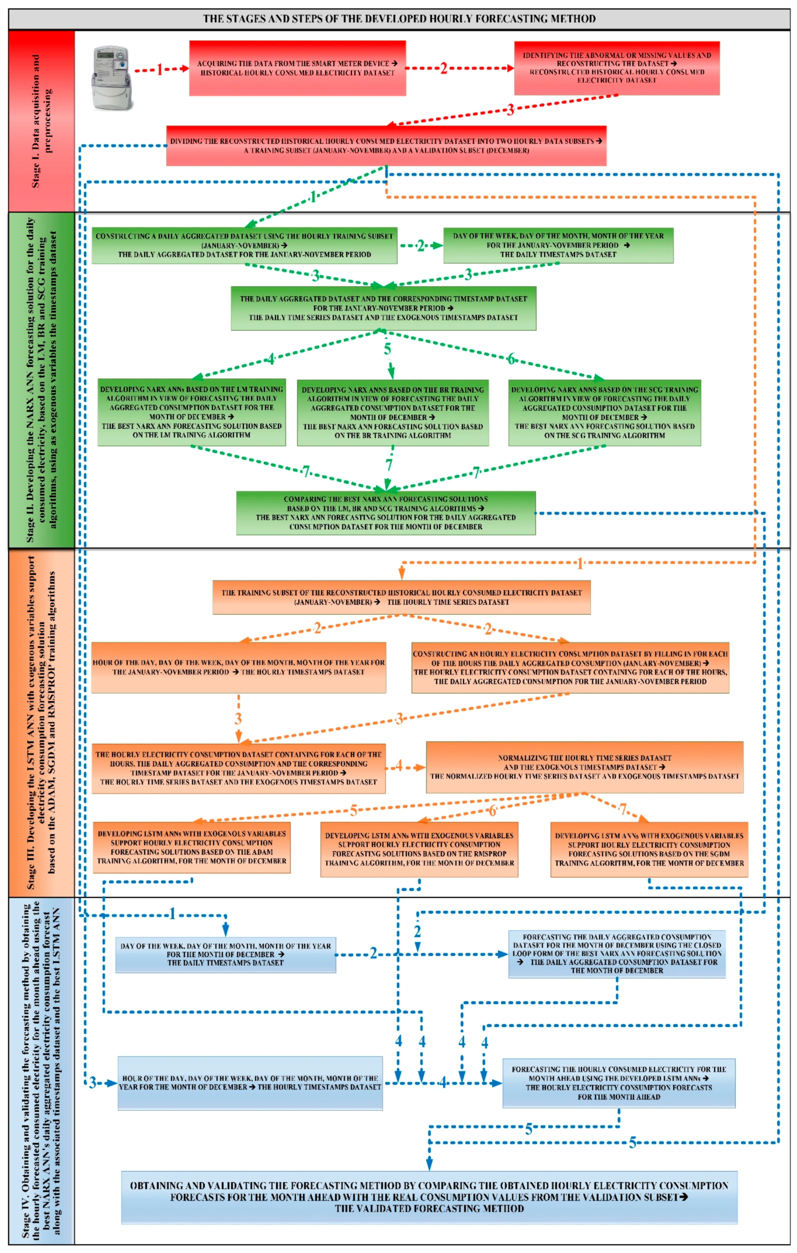
In the following, details regarding the stages and steps comprised by the developed forecasting method are presented.

2.3. Stage I: Data Acquisition and Preprocessing

During the first stage of the devised forecasting method that comprises three steps, in the first step we acquired the dataset, provided by the medium industrial electricity consumer who retrieved them from the smart metering device. The dataset consisted of 8760 records representing the hourly electricity consumption dataset corresponding to the year 2018, measured in MW h.

Afterwards, in the second step of this stage, taking into account the fact that sometimes one might encounter abnormal or missing values in the dataset (caused due to smart metering device’s recording errors or malfunctioning), we searched these values in order to reconstruct the historical hourly consumed electricity dataset. In the specific case of the analyzed medium industrial consumer, for the period to which the recorded data correspond, these kinds of values were not encountered, but due to the fact that the forecasting method targeted a wider range of medium industrial consumers posing similar characteristics, in order to be able to generalize the proposed approach, this step has been designed to manage the situations in which such values could appear. In this purpose, during this stage, we applied a gap-filling method based on the linear interpolation that provided reliable results when it has been developed and applied in previous studies that have been conducted along with my research team [25,26,32].

An important issue that has to be taken into account when one applies the filling method consists of identifying a particular threshold concerning the number of missing values (particularly the ones that are consecutive) which, when surpassed, can affect the training processes of the ANNs in terms of forecasting accuracy. In order to test the efficiency of the gap filling technique and to identify the above-mentioned threshold, we deleted on purpose several consecutive values from the electricity consumption dataset and, after applying the filling technique and using the developed forecasting method, it was remarked that the accuracy of the devised forecasting method was affected for a threshold consisting 16 or more consecutive missing values, especially when the missing values overlapped two consecutive days. In the case when the number of consecutive missing values would have surpassed the above-mentioned threshold, the efficiency of the filling method was lowered and therefore one should have to discard the missing or abnormal data altogether in the training process, if it had not been possible to acquire a new dataset from the contractor. In this case, as the dataset retrieved from the smart metering device had no missing or abnormal values and the medium industrial electricity consumer encountered no power outages within the considered period of one year, it was possible to use the whole hourly electricity consumption dataset, measured in MW h, consisting of 24 records per day, namely 8760 records corresponding to the year 2018.

In the third step of the first stage of the forecasting method, the reconstructed historical hourly consumed electricity dataset was divided into two data subsets, namely a training subset (representing the January–November period of the year 2018, consisting of 8016 samples) and a validation subset (representing the month of December of the year 2018, consisting of 744 samples). The first subset was used in developing, training, and validating the forecasting method, while the second one was put aside in order to obtain a final validation of the forecasting method through a comparison between the predicted hourly electricity consumption values for the month of December and the real, registered ones.

The contractor was a medium industrial electricity consumer from Romania that holds a bakery factory endowed with a flour mill, that produces pastries (such as bread, sweet bread, croissants, cornflakes, pretzels, pasta, biscuits, cakes, cookies), and has contracts with major retail stores, supermarket chains, and catering companies. Therefore, analyzing their specific activities, the quarterly sales reports, the local purchasing patterns and traditions, it was observed that, even in the national public holidays or winter holidays, the bakery factory’s work schedule was carried out in three work shifts.

Moreover, analyzing the Romanian eating habits, one can remark that bread is the most common consumed aliment and it is generally preferred at each meal, regardless of the category of population, if considering the age, gender, occupation, educational level and family type classification criteria. The report [50] states that in Romania the amount of bread consumption surpasses 95 kg per person per year, while in the rest of Europe the average yearly consumption is of about 60 kg per capita. Moreover, the same report remarks that the domestic bakery market in Romania (namely 1.1 billion Euro) represents more than 60% from the total Romanian bakery market (namely 1.8 billion Euro). Therefore, one can easily remark that the contractor’s activity is conducted continuously, working around the clock, in three shifts, regardless of the seasons, holidays, as its products are sold and bought daily by the Romanian customers.

A challenge that had to be overcome consisted of the fact that in Romania, in the year 2019, the smart metering devices’ implementation was still in an incipient phase and regardless of numerous legislative proposals [51], their adoption was made at a slow pace. Therefore, the dataset that has been registered and provided by the contractor contained the overall consumption at the bakery factory level, without having individual electricity consumption of different equipment used in the different stages of the production process available. Of particular interest for this research and also for the medium industrial electricity consumer was to obtain a method that can provide as accurate a forecast as possible of the hourly electricity consumption for the month-ahead.

Detailed information about the datasets can be found in the Supplementary Materials.

2.4. Stage II: Developing the NARX ANN Forecasting Solution for the Daily Consumed Electricity, Based on the LM, BR and SCG Training Algorithms, Using as Exogenous Variables the Timestamps Dataset

The second stage of the forecasting method comprises seven steps. In the first step of this stage, we constructed a daily aggregated electricity consumption dataset using the hourly training subset, therefore obtaining a subset of 334 samples, representing the daily electricity consumption for the January-November period of the year 2018.

Subsequently, in the second step of this stage, a daily timestamp dataset corresponding to the daily aggregated electricity consumption dataset was constructed, comprising of, for each of the above-mentioned 334 samples, the day of the week (denoted from 1 to 7, where 1 corresponds to the first day of the week, Monday), the day of the month (denoted from 1 to the number of days of the respective month, which can be 28, 30 or 31) and the month (denoted from 1 to 11, where 1 corresponds to the month of January and 11 to the month of November).

In the next step of the second stage, the third one, there are concatenated the daily aggregated dataset for the January–November period of the year 2018 and its associated timestamps dataset.

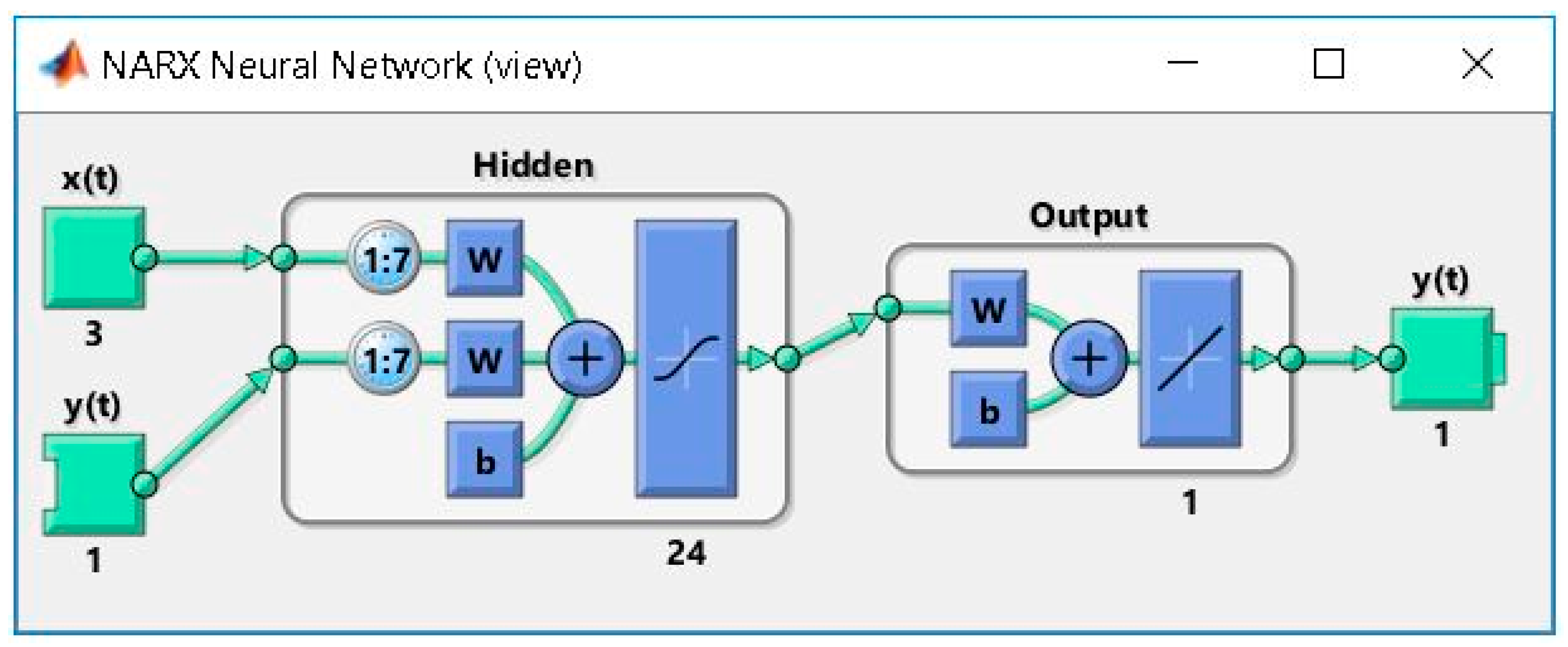
During the steps 4, 5 and 6 of the second stage we developed a series of ANNs forecasting solutions based on the NARX model, testing different settings and configurations regarding the employed training algorithm (Levenberg–Marquardt, Bayesian regularization, scaled conjugate gradient), the number of neurons from the hidden layer (n) and the value of the delay parameter (d). In the case of the NARX ANNs one employs not only the previous time series values but also additional, external values of another time series, the exogenous variables, that exert an influence upon the initial time series. In this case, the datasets from step 3 have been used as input parameters, namely the daily aggregated dataset for the January–November period of the year 2018 is used as time series, while its associated timestamps dataset is used as exogenous variables.

For each of the three above-mentioned training algorithms (LM, BR and SCG), 16 ANNs have been developed in order to forecast the month-ahead daily consumed electricity, having various architectures, namely, four neurons for the input data (one neuron for the daily electricity consumption dataset, three neurons for the timestamps exogenous data), a hidden layer’s size of n neurons, where $n\in \left\{8,16,24,48\right\}$, the delay parameter taking the values $d\in \left\{7,14,21,28\right\}$, the output layer containing one neuron and also one neuron for the output data (measured in MW h).

In all the cases, for all the $\left(n,d\right)$ pairs, in developing the forecasting NARX ANNs, for the LM and SCG training algorithms and the above-mentioned situations, the input dataset (comprising both the time series and the exogenous variables), containing 334 samples, has been divided according to the 70%—15%—15% approach, corresponding to the training, testing and validation processes, while in the case of the BR training algorithm the last 15% of the input dataset has not been allocated, because in this case the validation process does not take place. The decision to maintain unallocated this percentage is justified by the fact that in this way the dimension of the datasets used in the training and testing processes is the same, for all the three training algorithms, this fact assuring the relevance when comparing the obtained forecasting results.

Taking into consideration the fact that the input data has various ranges, in the purpose of minimizing the influence of these ranges on the obtained forecasted results, the normalization performance parameter has been set to the standard value, in this way ensuring the fact that the development environment considers the output elements as ranging in the interval $\left[-1,1\right]$ and computes the errors in accordance [52].

For each case we computed 30 training iterations, within which the samples corresponding to the above-mentioned percentages have been randomly allocated, the weights and biases of the NARX ANNs being re-initialized each time when the data from the percentages were re-allocated. When developing forecasting artificial neural networks, one should train them as to learn and perform certain tasks, based on specific training algorithms. In order to identify the most advantageous training algorithm, one should take into account both the forecasting accuracy and the training time criteria, the best training algorithm being characteristic to each specific case and problem, depending on many factors (the complexity of the analyzed problem, the network’s complexity and its specific architecture, the training set’s dimension, the weights and biases of the network, the desired level of accuracy, the previously specified level of accepted error, the training error’s purpose).

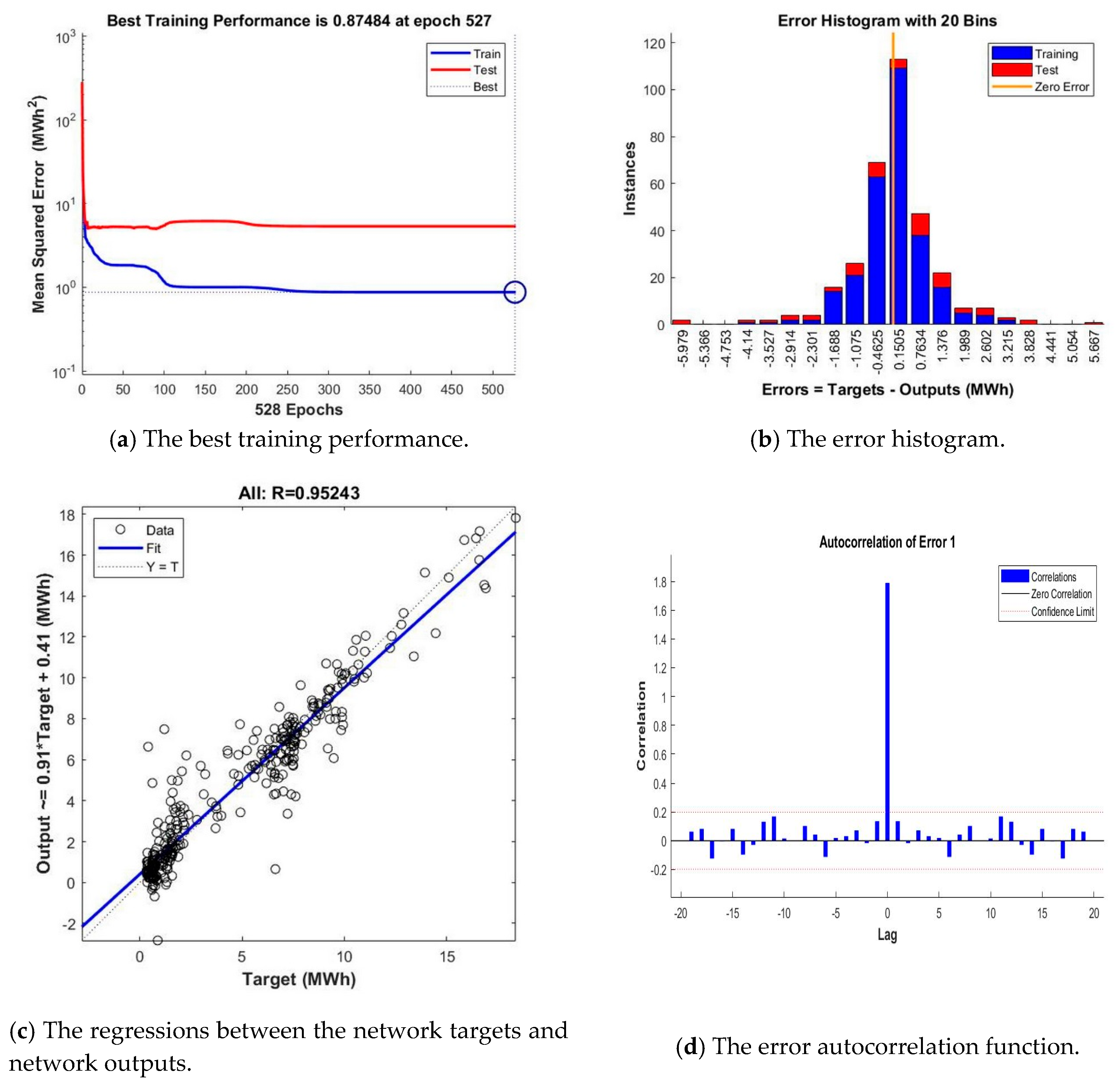
The training time represents a particularly important aspect that should be considered in evaluating the performance of the developed ANN-based forecasting solution, because when this solution is put into operation, the neural networks necessitate subsequent re-training procedures due to the fact that over the course of time, new datasets that contain timestamps are registered and provided as new inputs for the developed ANNs. Therefore, in assessing the networks’ performance, along with the performance metrics, the registered training times have also been taken into consideration. Regarding the 30 training iterations, there were recorded different results in terms of forecasting accuracy highlighted by the training times and the performance metrics, namely the MSE, R, the error histogram, the error autocorrelation, based on which the best NARX ANN has been identified and saved, while discarding the others. In this way, we identified and saved 16 NARX ANNs for each of the three training algorithms, therefore a total number of 48 neural networks. Afterwards, for each training algorithm was identified the best NARX ANN forecasting solution by comparing the registered training times and the values of the above-mentioned performance metrics, while the remaining networks, providing lower accuracies, have been discarded.

In the final step of the second stage, the seventh, the forecasting accuracies of the three NARX ANNs identified in the previous three steps, developed based on the three training algorithms (LM, BR and SCG), were assessed by comparing the registered training times and the above-mentioned performance metrics. Consequently, the best NARX ANN forecasting solution for the daily aggregated consumption dataset for the month-ahead has been identified, while the other two networks were discarded.

2.5. Stage III: Developing the LSTM ANN with Exogenous Variables Support Electricity Consumption Forecasting Solution Based on the ADAM, SGDM and RMSPROP Training Algorithms

The third stage of the devised hourly forecasting method for the month-ahead takes place over the course of seven steps. In the first step of this stage, we retrieved the training subset constructed in the last step of the first stage, representing the hourly consumed electricity dataset for the January–November period of the year 2018, consisting in 8016 samples.

Afterwards, in the second step of the third stage, we constructed an hourly timestamp dataset that matches the moments of time when the values of the above-mentioned dataset have been registered, comprising for each of the 8016 samples, the following elements: the hour of the day (denoted from 1 to 24), the day of the week (denoted from 1 to 7, where 1 corresponds to the first day of the week, Monday), the day of the month (denoted from 1 to the number of days of the respective month, which can be 28, 30 or 31) and the month (denoted from 1 to 11, where 1 corresponds to the month of January and 11 to the month of November). During the same step, we constructed an hourly electricity consumption dataset by filling in, for each of the hours, the daily aggregated consumption for the January-November period of the year 2018.

In the next step, the third one of the third stage, there are concatenated the hourly electricity consumption dataset containing for each of the hours, the daily aggregated electricity consumption for the January-November period of the year 2018, and its associated timestamps dataset.

According to the official development environment (MATLAB) documentation recommendations, in order to attain a better fitting and avoid the risk of a divergence during the training process, in the fourth step of this stage, the hourly time series dataset and its associated timestamps dataset have been normalized, processing the data as to have a variance of 1 and a 0 mean [53].

During the steps 5, 6 and 7 of the third stage, we developed a series of LSTM ANNs with exogenous variables support hourly electricity consumption forecasting solutions based on the ADAM, SGDM and RMSPROP training algorithms, using the datasets from step 4 as input parameters. Therefore, for each training algorithm, we developed 19 LSTM ANNs with exogenous variables support, in order to obtain in the subsequent stage the most accurate forecast of the hourly electricity consumption for the month-ahead, the networks having various architectures, namely 6 neurons for the sequence input layer (one neuron for the hourly electricity consumption dataset, 4 neurons for the timestamps exogenous data, one neuron for the aggregated electricity consumption dataset), a variable number of hidden units, $n\in \left\{10,20,\dots 100,200,\dots ,1000\right\}$, one neuron for the fully connected layer and a regression layer.

2.6. Stage IV: Obtaining and Validating the Forecasting Method by Obtaining the Hourly Forecasted Consumed Electricity for the Month Ahead Using the Best NARX ANN’s Daily Aggregated Electricity Consumption Forecast along with the Associated Timestamps Dataset and the Best LSTM ANN

During the first step of the fourth stage of the devised forecasting method that comprises five steps, we constructed a daily timestamp dataset for the month of December, containing 31 samples that comprise the day of the week (denoted from 1 to 7, where 1 corresponds to the first day of the week, Monday), the day of the month (ranging from 1 to 31) and the month (denoted with 12, corresponding to the month of December).

In the second step of this stage, using the closed loop form of the best NARX ANN forecasting solution identified and saved at the last step of Stage II and the daily timestamp dataset for the month of December, identified in the previous step of this stage, the daily aggregated consumption dataset for the month of December has been forecasted.

Afterwards, in the third step of the fourth stage, we constructed an hourly timestamp dataset for the month of December, comprising 744 samples that contain the hour of the day (denoted from 1 to 24), the day of the week (denoted from 1 to 7, where 1 corresponds to the first day of the week, Monday), the day of the month (ranging from 1 to 31) and the month (denoted with 12, corresponding to the month December).

In the fourth step of this stage, using the LSTM with exogenous variables support hourly electricity consumption forecasting ANNs developed based on the ADAM, SGDM and RMSPROP training algorithms, that have been previously developed in the last step of Stage III, along with the daily aggregated consumption dataset for the month of December that has been forecasted in the second step of the fourth stage and with the hourly timestamp dataset for the month of December constructed in the third step, in each case the hourly consumption dataset for the month of December has been forecasted, comprising of 744 samples.

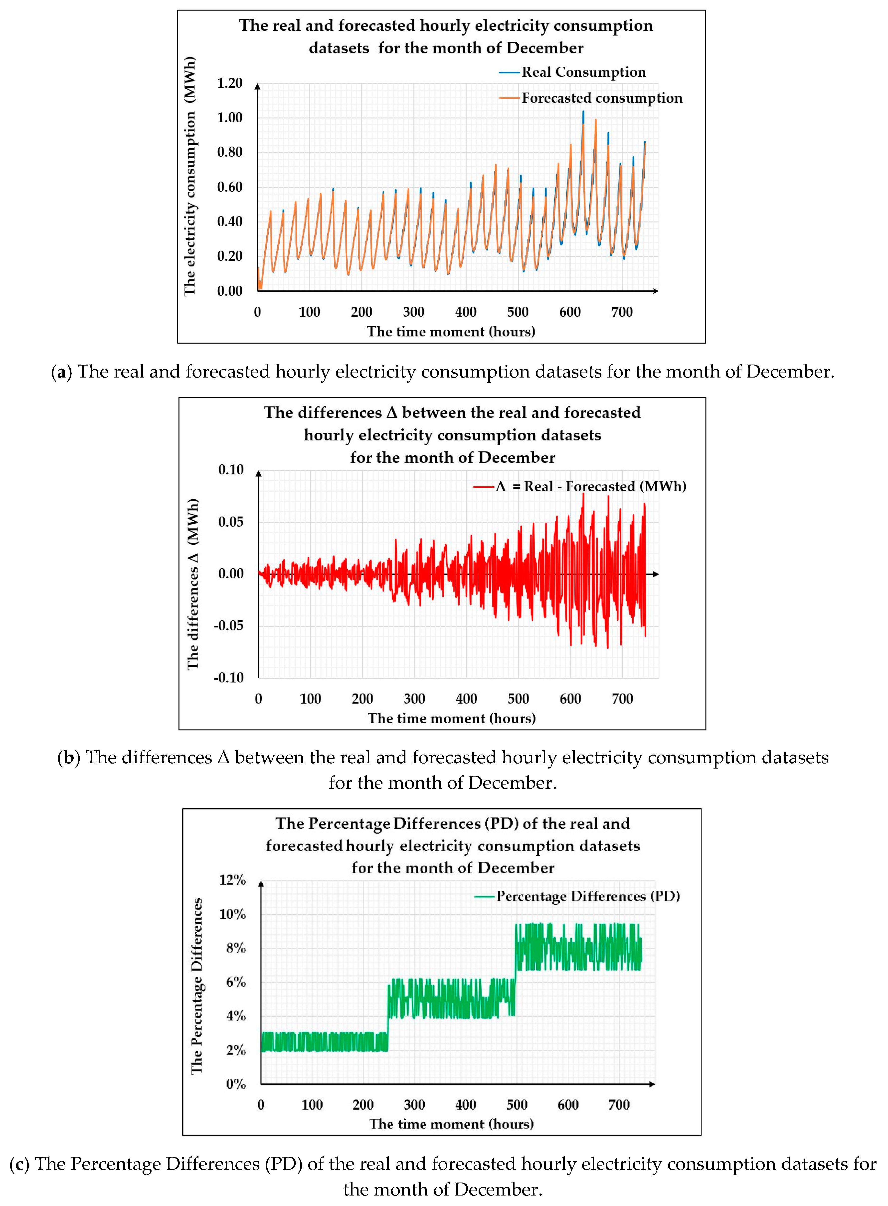
In the last step of this stage, the fifth, we obtained and validated the developed forecasting method by comparing the obtained hourly electricity consumption forecasts for the month-ahead with the real consumption values from the validation subset. In order to obtain a relevant comparison, during this stage, the differences between the real, registered values (stored in the validation dataset) and the forecasted ones corresponding to the hourly consumption dataset for the month of December, have been computed and evaluated.

According to the same methodology as in the case of the NARX ANNs, for each training algorithm and each number of hidden units, we computed 30 training iterations and, by comparing the registered training times and the values of the RMSE performance metric computed using the predicted values and the real ones, the best LSTM ANNs with exogenous variables support have been identified and saved for each training algorithm and value of n, while discarding the others. Each time when the networks have been retrained, during the 30 iterations, the training set has been divided in a random manner and therefore we minimized the influence that one could have obtained if the minibatches corresponding to the large dimension training dataset had been allocated incorrectly.

In this way, we saved 19 LSTM ANNs with exogenous variables support for each of the three training algorithms, therefore a total number of 57 neural networks. Afterwards, for each training algorithm, we identified and saved the best LSTM ANN forecasting solution by comparing the registered training times and the values of the above-mentioned performance metric, while the remaining networks, providing lower accuracies, have been discarded.

Afterwards, the forecasting accuracies of the three LSTM ANNs with exogenous variables support previously identified, developed based on the three training algorithms have been assessed, by comparing the above-mentioned performance metrics. Consequently, the best LSTM ANN hourly electricity forecasting solution for the month-ahead has been identified, while the other two networks have been discarded.

The designed, developed and validated forecasting method, presented in the above Section 2.3, Section 2.4, Section 2.5 and Section 2.6 for the month-ahead hourly electricity consumption in the case of medium industrial consumers, which benefits from both the advantages of NARX model and LSTM neural networks, is synthesized in the following flowchart (Figure 1).

The next section depicts the results registered during the experimental tests and their significance.

3. Results

Using the hardware and software configurations along with the datasets presented within the Materials and Methods section, during the stages and steps of the developed forecasting method for the month-ahead hourly electricity consumption in the case of medium industrial consumers, we registered the main experimental results that are presented in the following.

3.1. Results Regarding the Developed NARX ANN Forecasting Solution for the Daily Consumed Electricity, Based on the LM, BR and SCG Training Algorithms, Using as Exogenous Variables the Timestamps Dataset

Following the above depicted forecasting approach, in the second stage of this method, we developed the ANN forecasting solution based on the NARX model, using as exogenous variables the timestamps dataset and the obtained results have been synthetized in

Table 1. The synthesis of the experimental results when developing the artificial neural networks (ANNs) forecasting solution based on the non-linear autoregressive with exogenous inputs (NARX) model, using as exogenous variables the time stamps datasets.

The Levenberg-Marquardt Training Algorithm
n	d	7	14	21	28
8	MSE	4.1641	6.8932	4.3769	7.1552
	R	0.92758	0.9048	0.83911	0.84852
	t	0:00:01	0:00:01	0:00:01	0:00:01
16	MSE	4.9337	7.7799	7.8676	7.0909
	R	0.8435	0.84282	0.89168	0.87829
	t	0:00:01	0:00:01	0:00:01	0:00:02
24	MSE	5.4864	11.2554	8.359	9.2342
	R	0.89777	0.87193	0.9092	0.88455
	t	0:00:02	0:00:04	0:00:02	0:00:03
48	MSE	10.7977	11.7325	8.0716	10.3163
	R	0.89707	0.73786	0.85211	0.87776
	t	0:00:02	0:00:03	0:00:06	0:00:09
The Bayesian Regularization Training Algorithm
n	d	7	14	21	28
8	MSE	1.1512	1.3781	0.76579	6.6775e-15
	R	0.9541	0.93581	0.9391	0.96283
	t	0:00:4	0:00:13	0:00:29	0:01:30
16	MSE	0.90573	0.99617	8.3426e-15	6.805e-15
	R	0.94455	0.94485	0.95088	0.93863
	t	0:00:30	0:01:22	0:02:18	0:07:41
24	MSE	0.87484	1.3337	0.26305	6.1172e-16
	R	0.95243	0.93679	0.93582	0.94781
	t	0:00:30	0:01:17	0:06:35	0:18:47
48	MSE	1.8527	0.9868	2.8138e-20	5.8693e-07
	R	0.92382	0.94174	0.93724	0.93084
	t	0:04:05	19:14	0:29:00	1:23:51
The Scaled Conjugate Gradient Training Algorithm
n	d	7	14	21	28
8	MSE	4.7514	4.528	5.9659	4.5885
	R	0.87621	0.88132	0.83012	0.88173
	t	0:00:01	0:00:03	0:00:02	0:00:02
16	MSE	4.5976	5.6459	4.5474	4.8432
	R	0.88406	0.86584	0.86211	0.79012
	t	0:00:01	0:00:03	0:00:02	0:00:02
24	MSE	6.2231	6.2634	4.3487	6.3891
	R	0.88626	0.90171	0.9103	0.87767
	t	0:00:02	0:00:03	0:00:02	0:00:02
48	MSE	6.4186	6.2747	10.912	11.493
	R	0.89967	0.88604	0.81098	0.79819
	t	0:00:03	0:00:03	0:00:03	0:00:04

that contains the training times $t$ (measured in hours, minutes and seconds) and the performance metrics, namely the MSE, R, registered during the various tests, for the three different training algorithms, considering a hidden layer’s size of n neurons, where $n\in \left\{8,16,24,48\right\}$, and a delay parameter $d\in \left\{7,14,21,28\right\}$.

Analyzing and comparing the results synthetized in Table 1, one can remark that in the case of the LM training algorithm, the best daily forecasting accuracy has been provided by the network comprising eight neurons in the hidden layer, using a delay parameter of 7, as in this case we registered the lowest value for the mean squared error (MSE = 4.1651), along with the highest value of the correlation coefficient computed for the whole dataset (R = 0.92758), the result being obtained in about a second. The worst forecasting accuracy has been registered when using 14 neurons in the hidden layer and a delay parameter of 48, because in this case we registered the highest value of the mean squared error, namely 11.7325, along with the lowest value of the correlation coefficient, R = 0.73786, the training time being of 3 s.

As regarding the BR training algorithm, the most accurate forecasting has been obtained when using the network that comprises 24 hidden neurons, a delay parameter of 7, case in which we registered the highest value of the correlation coefficient R = 0.95243, along with the lowest value of the MSE, namely 0.87484 and a training time of 30 s. In contrast to this, in all the cases of the BR ANNs developed using 21 or higher neurons in the hidden layer, even if the training time has remained acceptable, the overfitting phenomenon has occurred, and the training time has increased significantly (up to 83 min). As a specific characteristic of the ANNs developed based on the BR training algorithm, one can notice that generally in this case the registered training times are higher than in the case of the other two training algorithms, and the forecasting results in this case cover a wide range of results, starting from the best up to the worst one, when compared to all the other forecasting results.

In the case of the SCG training algorithm, the synthesis from Table 1 highlights the fact that the best daily forecasting accuracy has been provided by the ANN developed using 24 neurons in the hidden layer and a delay parameter of 21, case in which we registered the lowest value for the mean squared error (MSE = 4.3487) and the highest value of the correlation coefficient (R = 0.9103), the training time being 2 s. In contrast to these results, the worst ones have been registered in the case of the ANN developed when using 28 neurons in the hidden layer and a delay parameter of 48, as in this case the registered values of the performance metrics were MSE = 11.493, R = 0.79819, the training time being of 4 s.

In all the cases, for all the three different training algorithms, LM, BR and SCG, when one has tried to further increase the delay parameter, two main drawbacks have appeared: either the training time has increased significantly (particularly in the case of the BR algorithm), or the overfitting phenomenon has occurred. Moreover, even if the two drawbacks did not appear in certain cases, when increasing the delay over 28 days, one has observed an insignificant performance gain, that could be rather related to a favorable division of the dataset than to the value of the delay parameter.

Afterwards, according to the seventh step of Stage II of the developed forecasting method, the forecasting accuracies (highlighted by the performance metrics) of the three NARX ANNs identified at the previous three steps have been compared and, in this way, one has identified the forecasting network that offers the best forecasting accuracy, from the 48 ones synthetized in Table 1, namely the NARX ANN forecasting solution for the daily consumed electricity, developed based on the BR training algorithm, using as exogenous variables the timestamps dataset, with n = 24 neurons in the hidden layer and a delay parameter of d = 7, entitled BEST_NARX. The architecture of this NARX ANN is depicted in Figure 2.

In order to evaluate and highlight the forecasting accuracy of the BEST_NARX network, the performance plots corresponding to this network have been represented and analyzed (Figure 3). Thus, the best training performance is represented in Figure 3a, that describes the variation of the Mean Squared Error (MSE) during the training epochs, along the training and testing curves. The graph shows that the best training performance has been obtained at the epoch 527, case in which the MSE has registered the value 0.87484. Moreover, this plot highlights the fact that the training and testing curves do not increase after reaching their convergence and therefore one can state that the forecasting solution is stable. By comparing these curves, one can also notice that the testing curve does not tend to increase in a significant manner before the training one, in this way demonstrating that the BEST_NARX network does not overfit the data and this represents a strong argument in proving that this ANN has been trained in an efficient manner, based on an appropriate division of the dataset.

Subsequently, the error histogram corresponding to the BEST_NARX network, developed based on the BR training algorithm, using as exogenous variables the timestamps dataset, designed to forecast the daily consumed electricity for the month-ahead, has been computed and represented in Figure 3b. Analyzing this plot, one remarks that most of the errors range between −1.688 and 1.376, which represents a reduced size range, while only for a small number of training points, the errors are outside the above-mentioned range. In addition to this, the error histogram shows that the majority of the errors are around a very small value, namely 0.1505.

Afterwards, the regressions between the network targets and network outputs in the case of the BEST_NARX network were computed and plotted in Figure 3c that highlights the obtained values of the correlation coefficient, which were higher than 0.95243, therefore close to the value 1. As a consequence, analyzing this plot, one can conclude that the NARX artificial neural network developed based on the BR training algorithm, using as exogenous variables the timestamps dataset, with n = 24 neurons in the hidden layer and a delay parameter of d = 7 offers a very good matching between the targets and outputs of the network.

Finally, the error autocorrelation function corresponding to the BEST_NARX network has been represented in Figure 3d. This plot highlights the way in which the forecasting errors of this network are interlinked during the time and, by analyzing it, one remarks that apart from the correlation characterized by zero-lag, all the others fall inside the desired confidence limits around zero.

The performance plots detailed above confirm the increased forecasting accuracy of the BEST_NARX ANN, thus proving the advantages of choosing this network in view of obtaining a daily forecasting solution for the month-ahead consumed electricity.

One can find in the Supplementary Materials file the developed NARX ANN that has registered the best results, namely the BEST_NARX network.

3.2. Results Regarding the Developed LSTM ANNs with Exogenous Variables Support Electricity Consumption Forecasting Solution Based on the ADAM, SGDM and RMSPROP Training Algorithms

In the Stage III of the presented methodology, in order to obtain an hourly electricity consumption forecasting solution for the month of December, we developed a LSTM ANNs with exogenous variables support electricity consumption forecasting solution based on the ADAM, SGDM and RMSPROP training algorithms. Afterwards, in Stage IV, we obtained and validated the forecasting method by computing the hourly forecasted consumed electricity for the month-ahead, using the best NARX ANN’s daily aggregated electricity consumption forecast along with the associated timestamps dataset and the LSTM ANNs developed in steps 5, 6 and 7 of the Stage III.

Based on the selection criteria regarding the 30 training iterations described in Stage IV, we selected the best LSTM ANNs for each training algorithm and each dimension of the hidden layer. The results obtained according to the devised forecasting method have been synthetized in

Table 2. The synthesis of the experimental results registered for the 19 developed long short-term memory (LSTM) ANNs per each training algorithm.

No.	Hidden Units	The Training Algorithm
		ADAM		SGDM		RMSPROP
		RMSE	Running Time	RMSE	Running Time	RMSE	Running Time
1	10	4.2944	117	1.9083	131	4.3997	148
2	20	3.2567	117	1.9911	120	0.3185	147
3	30	0.1092	117	2.1446	124	0.0720	145
4	40	0.1002	117	1.7767	124	0.1250	144
5	50	0.0834	117	2.3133	123	0.0766	146
6	60	0.1812	117	2.1498	124	0.2389	146
7	70	0.2301	121	2.2111	120	0.1490	152
8	80	0.1450	122	2.2327	124	0.2461	143
9	90	0.2702	120	2.5335	120	0.1019	147
10	100	0.2630	132	2.4265	138	0.3621	128
11	200	0.2628	156	2.5167	129	0.2856	151
12	300	0.2660	259	2.6352	136	0.2495	159
13	400	0.0244	379	2.4944	152	0.2264	168
14	500	0.2139	552	2.4152	233	0.3035	251
15	600	0.1504	588	2.9985	246	0.2324	263
16	700	0.3241	757	3.4813	297	0.3475	302
17	800	0.3415	923	3.7986	301	0.3430	322
18	900	0.3278	1181	3.6595	619	0.3448	406
19	1000	0.2630	1394	3.7831	456	0.3432	465

that contains the running times t (measured in seconds) and the performance metric, namely the RMSE, registered during the various tests, for the three different training algorithms, considering the dimension of the hidden layer $n\in \left\{10,20,\dots ,100,200,\dots ,1000\right\}$, therefore developing 19 LSTM ANNs in each case.

The results synthetized in Table 1 show that most of the LSTM ANNs from the 57 presented in this table offer a very good forecasting accuracy and therefore they can be successfully put into operation in a real production environment. However, one must remark that by increasing the number of hidden units, the running time increased significantly without bringing an improvement regarding the forecasting accuracy. On the contrary, when the number of hidden units exceeded the value of 1000, an overfitting process occurred and therefore the experimental tests had to be developed limiting the dimension of the hidden layer at 1000.

By comparing the registered results in the case of the 19 LSTM ANNs developed using the ADAM training algorithm, one remarks that the best prediction results in terms of accuracy are provided by the network developed using 400 hidden units, case in which the value of RMSE is 0.0244, while the registered running time is 379 s. This reduced amount of time represents an advantage for the moment when the forecasting solution is put into operation and the ANNs must be retrained, in order to use the new acquired input datasets.

Based on the same approach, comparing the 19 LSTM ANNs trained using the SGDM algorithm, one has identified the network that has provided the best forecasting accuracy, namely the one developed using 40 hidden units, when RMSE had the value 1.7767 and the running time has been 124 s.

Using the same type of comparison, starting from the results registered for the 19 LSTM ANNs developed based on the RMSPROP training algorithm, one observes that the best forecasting accuracy has been provided by the network having 30 hidden units, for which we registered the lowest value of the RMSE, namely 0.0720, along with a running time of 145 s.

Afterwards, according to the devised approach, by comparing the forecasting accuracy of the three selected LSTM ANNs, developed based on the three training algorithms, ADAM, SGDM and RMSPROP, one concludes that the best prediction accuracy, highlighted by the lowest value of the RMSE performance metric, was registered by the network trained using the ADAM algorithm, using 400 hidden units, entitled BEST_LSTM. The architecture of this LSTM ANN is depicted in Figure 4.

One can find in the Supplementary Materials file the developed LSTM ANN that has registered the best results, namely the BEST_LSTM network.

3.3. Results Regarding the Validation of the Forecasting Method by Comparing the Obtained Hourly Electricity Consumption Forecasts for the Month Ahead with the Real Consumption Values from the Validation Subset

During the fifth step of the fourth stage of the developed forecasting method, in order to obtain and validate this method, the hourly electricity consumption forecasts for the month-ahead have been compared with the real consumption values from the validation subset. In this way, one can assess the forecasting accuracy of the method, assessment that is very useful in deciding if the developed method is suitable to be implemented in a real production environment. For this purpose, the devised method has been applied, using the two previously developed, identified and saved artificial neural networks (BEST_NARX for obtaining the month-ahead daily aggregated consumption dataset and BEST_LSTM for obtaining the month-ahead hourly consumption dataset) and afterwards, the forecasted month-ahead hourly consumption dataset has been compared with the real consumption one, stored in the validation subset.

In order to obtain a relevant, appropriate comparison, the plots of the real and forecasted hourly electricity datasets for the month-ahead have been represented on the same chart (Figure 5a). This plot shows that the two curves have the same trend and very close values, which confirms the very good forecasting accuracy of the developed method. With the aim of refining the comparison, there have also been computed and represented the differences Δ (Figure 5b) and the percentage differences PD (Figure 5c) between the real and forecasted hourly electricity consumption datasets for the month-ahead. The plots highlight the fact that these differences are very small during the first ten days (240 h), increasing gradually for the next ten days and even more in the last 11 days of the month of December, but still remaining sufficiently low as to be used by the contractor. Therefore, one can conclude that the forecasting accuracy was extremely good in the first third part of the month, remaining very good in the second one and good in the last part of the forecasted month.

In the Supplementary Materials one can find comprehensive details regarding the obtained results.

The obtained forecasted results, along with the performance metrics, the performance plots and the above-described comparison between the obtained hourly electricity consumption forecast for the month-ahead and the real consumption values from the validation subset, lead to the validation of the developed forecasting method, which proves to be an accurate and useful tool for obtaining the hourly electricity consumption forecast for the month-ahead.

In what follows, a discussion regarding the obtained forecasting results is presented, focusing on their interpretation in perspective of previous studies and methods from the scientific literature regarding similar problems.

4. Discussion

The decision to devise the above-described forecasting method has as main starting points the recent technical evolution and development of the CUDA architecture along with the fact that a wide range of state-of-the-art artificial intelligence development tools offered by professional development environments allow the harnessing of the huge parallel processing capability of the CUDA architecture. Therefore, based on these arguments, the forecasting method has been developed for the month-ahead hourly electricity consumption in the case of medium industrial consumers, by making use in different processing stages of the method, of the excellent forecasting capabilities of both NARX and LSTM ANNs with exogenous variables support, overcoming what would have been not long ago a huge computational cost affecting the necessary time to train and retrain the ANNs.

As stated and proved within the validation stage, the devised forecasting method offers an excellent forecasting accuracy. However, a mandatory comparison that should be made in order to justify the devised approach consists in evaluating the performance of the NARX and LSTM artificial neural networks, considering each of them as separate individual forecasting methods for the month-ahead hourly electricity consumption in the case of medium industrial consumers, based on the same case study, namely the one of the bakery factory.

For this purpose, firstly we developed an approach based only on the NARX ANNs (entitled NARX_ONLY), using the same hourly dataset, the same division into training and validation subsets, the same hourly timestamps dataset as exogenous variables, the same training algorithms (LM, BR and SCG) and the same number of training iterations like in the developed forecasting method’s case. In all the cases, the registered forecasting results were considerably lower than the ones of the developed approach, for example in the case of the best NARX ANN developed using the BR training algorithm, comprising 24 hidden neurons and having a delay parameter of 7, the registered value of the RMSE is 0.2513. As mentioned previously, in the developed forecasting method, in the best identified case, we registered a RMSE value of 0.0244, which is more than 10 times lower than in the case of the method developed based solely on the NARX ANN.

Secondly, an approach has been developed based solely on the LSTM ANNs (entitled LSTM_ONLY), using the same hourly dataset, the same hourly timestamps dataset as exogenous variables, the same training algorithms (ADAM, SGDM and RMSPROP) and the same number of training iterations like in the case of the developed forecasting method. In all the situations, the registered forecasting results were considerably lower than the ones provided by the developed approach, for example in the case of the best LSTM ANN developed using the ADAM training algorithm, comprising 400 hidden units, the registered value of the RMSE is 0.4103. As mentioned previously, in the developed forecasting method, in the best identified case we registered the value of 0.0244 for the RMSE performance metric, which is more than 16 times lower than in the case of the method developed based solely on the LSTM ANN.

For the two mentioned examples, the two cases analyzed above along with the comparison to the developed forecasting method are synthetized in

Table 3. The synthesis of the experimental results registered for the developed forecasting method and for the separate NARX and LSTM ANNs.

The Values of The Root Mean Square Error and Their Comparison
The Forecasting Method
The developed method, considering: for NARX: BR training algorithm, n = 24, d = 7 (BEST_NARX ANN) for LSTM: ADAM training algorithm, 400 hidden units (BEST_LSTM ANN)	NARX_ONLY, considering: BR training algorithm, n = 24, d = 7	LSTM_ONLY, considering: ADAM training algorithm, 400 hidden units
0.0244	0.2513	0.4103
Comparison: the ratio between the RMSE in each case of other forecasting methods and the one of the proposed forecasting method	10.29	16.81

.

Based on these remarks, one can state that the devised forecasting method that benefits in different processing stages from the forecasting capabilities of both NARX and LSTM ANNs with exogenous variables support, outperforms each of the NARX and LSTM artificial neural networks, considering them as separate approaches for the month-ahead hourly electricity consumption in the case of medium industrial consumers.

After developing the method from this paper, the NARX_ONLY and the LSTM_ONLY approaches, three more approaches for predicting the month-ahead hourly electricity consumption in the case of medium industrial consumers have been developed, in order to compare them with the approach developed within the current paper.

When compared to the study developed in [26] along with members of my research group, a scientific article within which forecasting solutions regarding electricity consumption in the case of commercial center type consumers have been developed, in the current paper another type of customer is approached, having a different electricity consumption profile. As the forecasting methods from the previous paper (based on NAR and NARX models) did not offer satisfactory results in the case of a medium industrial consumer, the forecasting method developed in the current study has been developed based on a different approach, employing in its different stages NARX along with LSTM artificial neural networks. Moreover, even if in both papers the purpose was to obtain a month-ahead accurate hourly consumption, in the case of the commercial center type consumer research, the exogenous data that have been used in developing the NARX ANNs consisted in both a timestamps dataset and a meteorological dataset (containing the outdoor temperature), while in the case of the current study we used as exogenous variables only a timestamps dataset, for both the LSTM and NARX ANNs. The increased obtained forecasting accuracy of the developed method represents an advantage for the industrial contractor, as in using the devised approach he will not have to purchase daily meteorological forecasts for the geographic area within which the bakery factory is located.

A wide range of papers from the scientific literature analyze issues regarding the industrial electricity consumption, developing various approaches, targeting the specific of the consumer and the desired type of forecasting. In this purpose, the researchers used different approaches and optimizations techniques, like: the grey model [6,14], SVM models [7,15], linear regression techniques [7], Markov chains [8,11], AdaBoost, ESN, FOA techniques [10], bottom-up approach combined with the linear hierarchical models [11], GA, PSO and BPNN [12], Granger causality and partial Grainger causality networks [13], LSSVM enriched using a MCC [15], while the current paper develops an approach based on the NARX along with LSTM artificial neural networks. Analyzing the forecast time horizon of the developed approaches from the literature, one can remark that the prediction horizon in the case of the industrial consumer varies in accordance to the necessities and requests of the industrial operator, ranging from short-term [7,12] up to medium [17] and long-term [11], in this last category being also comprised the developed forecasting method from the current paper. With respect to the obtained results, obviously each approach is tailored for its specific problem and therefore a relevant comparison between the approaches cannot be devised without taking into consideration the fact that these studies use different datasets and target different final purposes. However, one can state that all the approaches provide very good results in terms of forecasting accuracy, fulfilling the purposes for which they were developed and bringing real benefits to the beneficiaries.

Even if the obtained forecasting results highlighted by the performance metrics, the performance plots, the comparison between the real consumption and the forecasted one, allow one to consider the devised forecasting method as an accurate, useful tool for obtaining the hourly electricity consumption forecast for the month-ahead, the developed approach still has its limitations, and the most prominent one is the fact that it requires historical data for at least 11 months in order to obtain an hourly forecast for the month-ahead, otherwise the forecasting results are not consistent and reliable.

Considering the increased reluctance of the industrial operators to provide and share with one another data regarding their activity, including the electricity consumption, future work consists in prospecting the possibility of applying an encryption technique, namely the multilayered structural data sectors switching algorithm [54] in view of convincing the industrial operators to share their data and take advantage of a larger data pool, from several industrial operators, while maintaining their own sensible information private and secure.

As a result of performing an in-depth study of the scientific literature, one can remark that there are numerous scientists who have devoted their work on forecasting accurately the electricity consumption of industrial consumers and of the industrial sector as a whole, aiming to devise an extensive diversity of prediction methods targeted at certain case studies. Devising an exhaustive comparison with regard to the significant aspects of the various methods is a hard to attain task, all the more so an unattainable one, considering the wide variety of case studies, datasets and objectives that all of this research involves. Nevertheless, when particular targeted problems pose certain characteristics in common, it becomes conceivable for a method to be adjusted fittingly from one particular case to another, during the course of a generalizing process. The bakery factory on which the developed forecasting method has been applied to, is a non-limitative case of putting into practice the developed forecasting method, considering the fact that the industrial consumer is a representative case for other operating industrial consumers that are categorized from the electricity consumption point of view by the European Regulations in the same Band-IC category [55].

In view of this perspective, the forecasting method for the month-ahead hourly electricity consumption in the case of medium industrial consumers, devised, developed and validated according to the presented methodology from Section 2, can be applied successfully, and to that end, generalized to further case studies posing similar characteristics to the analyzed one. In addition, the proposed prediction method has been developed and compiled in a state-of-art development environment, being able to be implemented in a wide range of forecasting applications, assuring its install-ability, modularity, adaptability, reusability and changeability characteristics from the software quality point of view, particular features that substantiate the generalization capability also from the software implementation perspective, consequently highlighting the efficiency of the proposed approach.

5. Conclusions

The objective of this paper, namely the obtaining of an accurate forecast of the hourly electricity consumption for the medium industrial consumers, represents a subject of particular importance to industrial consumers and system operators alike. The accurate prediction of the industrial consumers’ electricity needs allows them to devise cost-effective production plans in terms of electricity consumption, while maximizing their productivity, therefore providing valuable decision support information with regard to their energetic needs. Moreover, an accurate month-ahead hourly electricity consumption forecast represents for the industrial consumers an increased opportunity in implementing intelligent energy management strategies, assuring an efficient economic scheduling of their resources, offering them the possibility to negotiate in advance appropriate billing tariffs that rely on accurate hourly forecasts, in the same time facilitating an optimal energy management for dispatch operators.

The forecasting approach designed, developed and validated in this paper succeeded to predict the month-ahead hourly electricity consumption in the case of medium industrial consumers, harnessing both the NARX’s advantages in terms of forecasting accuracy when predicting the daily electricity consumption and the LSTM’s advantages in terms of learning long-term dependencies useful for refining the resolution of the daily forecast up to an hourly level.

The analysis of the obtained experimental results, the validation of the developed forecasting method, the comparison of the devised method with other forecasting approaches from the scientific literature, represent valid arguments that highlight the contribution of the proposed approach in narrowing the gap identified within the body of knowledge, namely the need of a high-accuracy forecasting method for the month-ahead hourly electricity consumption in the case of medium industrial consumers.

Although the developed forecasting method targets medium industrial consumers, its accuracy and generalization capability make it a potential useful tool in view of promoting innovative business models with regard to industrial consumers that intend to sustain a part of the electricity consumption using renewable energy resources, consequently reducing their expenses related to electricity.

References

1. Exxon Mobil, 2018 Outlook for Energy: A View to 2040. Available online: https://corporate.exxonmobil.com/en/~/media/Global/Files/outlook-for-energy/2018-Outlook-for-Energy.pdf (accessed on 5 May 2019).
2. International Energy Agency. World Energy Outlook 2018. Executive Summary. Available online: https://webstore.iea.org/download/summary/190?fileName=English-WEO-2018-ES.pdf (accessed on 5 May 2019).
3. International Energy Agency. Global Energy and CO2 Status Report. Available online: https://www.iea.org/geco/electricity/ (accessed on 5 May 2019).
4. Index Mundi. Available online: https://www.indexmundi.com/g/g.aspx?c=xx&v=81 (accessed on 5 May 2019).
5. National Energy Regulatory Authority, National Report Issued on 31 July 2018. Available online: https://www.anre.ro/ro/despre-anre/rapoarte-anuale (accessed on 5 May 2019).
6. Wang, Z.X.; Hao, P. An improved grey multivariable model for predicting industrial energy consumption in China. Appl. Math. Model. 2016, 40, 5745–5758. [Google Scholar] [CrossRef]
7. Bracale, A.; Carpinelli, G.; De Falco, P.; Hong, T. Short-term industrial reactive power forecasting. Int. J. Electr. Power 2019, 107, 177–185. [Google Scholar] [CrossRef]
8. Berk, K.; Hoffmann, A.; Müller, A. Probabilistic forecasting of industrial electricity load with regime switching behavior. Int. J. Forecast. 2018, 34, 147–162. [Google Scholar]
9. De Oliveira, E.M.; Oliveira, F.L.C. Forecasting mid-long term electric energy consumption through bagging ARIMA and exponential smoothing methods. Energy 2018, 144, 776–788. [Google Scholar] [CrossRef]
10. Wang, L.; Lv, S.X.; Zeng, Y.R. Effective sparse adaboost method with ESN and FOA for industrial electricity consumption forecasting in China. Energy 2018, 155, 1013–1031. [Google Scholar] [CrossRef]
11. Da Silva, F.L.C.; Oliveira, F.L.C.; Souza, R.C. A bottom-up bayesian extension for long term electricity consumption forecasting. Energy 2019, 167, 198–210. [Google Scholar] [CrossRef]
12. Hu, Y.; Li, J.; Hong, M.; Ren, J.; Lin, R.; Liu, Y.; Liu, M.; Man, Y. Short term electric load forecasting model and its verification for process industrial enterprises based on hybrid GA-PSO-BPNN algorithm—A case study of papermaking process. Energy 2019, 170, 1215–1227. [Google Scholar] [CrossRef]
13. Yao, C.Z.; Lin, Q.W.; Lin, J.N. A study of industrial electricity consumption based on partial Granger causality network. Phys. A Stat. Mech. Appl. 2016, 461, 629–646. [Google Scholar] [CrossRef]
14. Ding, S.; Hipel, K.W.; Dang, Y.-g. Forecasting China’s electricity consumption using a new grey prediction model. Energy 2018, 149, 314–328. [Google Scholar] [CrossRef]
15. Duan, J.; Qiu, X.; Ma, W.; Tian, X.; Shang, D. Electricity consumption forecasting scheme via improved LSSVM with maximum correntropy criterion. Entropy 2018, 20, 112. [Google Scholar] [CrossRef]
16. Amber, K.P.; Ahmad, R.; Aslam, M.W.; Kousar, A.; Usman, M.; Khan, M.S. Intelligent techniques for forecasting electricity consumption of buildings. Energy 2018, 157, 886–893. [Google Scholar] [CrossRef]
17. Guo, H.; Chen, Q.; Xia, Q.; Kang, C.; Zhang, X. A monthly electricity consumption forecasting method based on vector error correction model and self-adaptive screening method. Int. J. Electr. Power Energy Syst. 2018, 95, 427–439. [Google Scholar] [CrossRef]
18. Abbas, F.; Feng, D.; Habib, S.; Rahman, U.; Rasool, A.; Yan, Z. Short term residential load forecasting: An Improved optimal nonlinear auto regressive (NARX) method with exponential weight decay function. Electronics 2018, 7, 432. [Google Scholar] [CrossRef]
19. Zahid, M.; Ahmed, F.; Javaid, N.; Abbasi, R.A.; Zainab Kazmi, H.S.; Javaid, A.; Bilal, M.; Akbar, M.; Ilahi, M. Electricity price and load forecasting using enhanced convolutional neural network and enhanced support vector regression in smart grids. Electronics 2019, 8, 122. [Google Scholar] [CrossRef]
20. Divina, F.; Gilson, A.; Goméz-Vela, F.; Torres, M.G.; Torres, J.F. Stacking ensemble learning for short-term electricity consumption forecasting. Energies 2018, 11, 949. [Google Scholar] [CrossRef]
21. Khuntia, S.R.; Rueda, J.L.; Van der Meijden, M.A. Long-term electricity load forecasting considering volatility using multiplicative error model. Energies 2018, 11, 3308. [Google Scholar] [CrossRef]
22. Xu, L.; Li, C.; Xie, X.; Zhang, G. Long-short-term memory network based hybrid model for short-term electrical load forecasting. Information 2018, 9, 165. [Google Scholar] [CrossRef]
23. Li, K.; Zhang, T. Forecasting electricity consumption using an improved grey prediction model. Information 2018, 9, 204. [Google Scholar] [CrossRef]
24. Mujeeb, S.; Javaid, N.; Ilahi, M.; Wadud, Z.; Ishmanov, F.; Afzal, M.K. Deep long short-term memory: A new price and load forecasting scheme for big data in smart cities. Sustainability 2019, 11, 987. [Google Scholar] [CrossRef]
25. Pîrjan, A.; Căruțașu, G.; Petroșanu, D.-M. Designing, developing, and implementing a forecasting method for the produced and consumed electricity in the case of small wind farms situated on quite complex hilly terrain. Energies 2018, 11, 2623. [Google Scholar] [CrossRef]
26. Pîrjan, A.; Oprea, S.-V.; Căruțașu, G.; Petroșanu, D.-M.; Bâra, A.; Coculescu, C. Devising hourly forecasting solutions regarding electricity consumption in the case of commercial center type consumers. Energies 2017, 10, 1727. [Google Scholar] [CrossRef]
27. Pîrjan, A. A mixed approach towards improving software performance of compute unified device architecture applications. J. Inf. Syst. Oper. Manag. 2017, 10, 448–459. [Google Scholar]
28. Smart-Optim. National Research Project. Title: Informatics Solutions for Electricity Consumption Analysis and Optimization in Smart Grids. Available online: https://sites.google.com/a/csie.ase.ro/smart-optim/home (accessed on 5 May 2019).
29. Lin, T.; Horne, B.G.; Tino, P.; Giles, C.L. Learning long-term dependencies in NARX recurrent neural networks. IEEE Trans. Neural Netw. 1996, 7, 1329–1338. [Google Scholar]
30. MathWorks Documentation. Choose a Multilayer Neural Network Training Function. Available online: https://www.mathworks.com/help/deeplearning/ug/choose-a-multilayer-neural-network-training-function.html;jsessionid=a03d2ad7477e1aa834eea7ff6d37 (accessed on 5 May 2019).
31. Kişi, Ö.; Uncuoǧlu, E. Comparison of three back-propagation training algorithms for two case studies. Indian J. Eng. Mater. Sci. 2005, 12, 434–442. [Google Scholar]
32. Oprea, S.-V.; Pîrjan, A.; Căruțașu, G.; Petroșanu, D.-M.; Bâra, A.; Stănică, J.-L.; Coculescu, C. Developing a mixed neural network approach to forecast the residential electricity consumption based on sensor recorded data. Sensors 2018, 18, 1443. [Google Scholar] [CrossRef]
33. Lungu, I.; Căruțașu, G.; Pîrjan, A.; Oprea, S.V.; Bara, A. A two-step forecasting solution and upscaling technique for small size wind farms located in hilly areas of Romania. Stud. Inform. Control 2016, 25, 77–86. [Google Scholar] [CrossRef]
34. Lungu, I.; Bâra, A.; Cărutasu, G.; Pîrjan, A.; Oprea, S.V. Prediction intelligent system in the field of renewable energies through neural networks. Econ. Comput. Econ. Cybern. Stud. Res. 2016, 50, 85–102. [Google Scholar]
35. MacKay, D.J.C. Bayesian interpolation. Neural Comput. 1992, 4, 415–447. [Google Scholar] [CrossRef]
36. Foresee, F.D.; Hagan, M.T. Guass-Newton approximation to bayesian learning. In Proceedings of the International Conference on Neural Networks, Houston, TX, USA, 9–12 June 1997; pp. 1930–1935. [Google Scholar]
37. Møller, M.F. A scaled conjugate gradient algorithm for fast supervised learning. Neural Netw. 1993, 6, 525–533. [Google Scholar] [CrossRef]
38. Hochreiter, S.; Schmidhuber, J. Long short-term memory. Neural Comput. 1997, 9, 1735–1780. [Google Scholar] [CrossRef]
39. Murad, A.; Pyun, J.-Y.; Murad, A.; Pyun, J.-Y. Deep recurrent neural networks for human activity recognition. Sensors 2017, 17, 2556. [Google Scholar] [CrossRef] [PubMed]
40. Zheng, H.; Yuan, J.; Chen, L.; Zheng, H.; Yuan, J.; Chen, L. Short-term load forecasting using EMD-LSTM neural networks with a Xgboost algorithm for feature importance evaluation. Energies 2017, 10, 1168. [Google Scholar] [CrossRef]
41. Nguyen, M.-T.; Nguyen, V.-H.; Yun, S.-J.; Kim, Y.-H. Recurrent neural network for partial discharge diagnosis in gas-insulated switchgear. Energies 2018, 11, 1202. [Google Scholar] [CrossRef]
42. Huang, C.-J.; Kuo, P.-H.; Huang, C.-J.; Kuo, P.-H. A deep CNN-LSTM model for particulate matter (PM2.5) forecasting in smart cities. Sensors 2018, 18, 2220. [Google Scholar] [CrossRef]
43. Bouktif, S.; Fiaz, A.; Ouni, A.; Serhani, M.M.A. Optimal deep learning LSTM model for electric load forecasting using feature selection and genetic algorithm: Comparison with machine learning approaches. Energies 2018, 11, 1636. [Google Scholar] [CrossRef]
44. Graves, A.; Liwicki, M.; Fernández, S.; Bertolami, R.; Bunke, H.; Schmidhuber, J. A novel connectionist system for unconstrained handwriting recognition. IEEE Trans. Pattern Anal. Mach. Intell. 2009, 31, 855–868. [Google Scholar] [CrossRef]
45. Hirschberg, J.; Manning, C.D. Advances in natural language processing. Science 2015, 349, 261–266. [Google Scholar] [CrossRef]
46. Xiong, W.; Droppo, J.; Huang, X.; Seide, F.; Seltzer, M.; Stolcke, A.; Yu, D.; Zweig, G. The Microsoft 2017, conversational speech recognition system. In Proceedings of the 2018 IEEE International Conference on Acoustics, Speech and Signal Processing (ICASSP), Calgary, AB, Canada, 15–20 April 2018. [Google Scholar]
47. Yue, B.; Fu, J.; Liang, J. Residual recurrent neural networks for learning sequential representations. Information 2018, 9, 56. [Google Scholar] [CrossRef]
48. Sutton, R.S. Two problems with backpropagation and other steepest-descent learning procedures for networks. In Proceedings of the Eighth Annual Conference of the Cognitive Science Society, Amherst, MA, USA, 15–17 August 1986. [Google Scholar]
49. Kingma, D.P.; Ba, J.L. Adam: A method for stochastic optimization. In Proceedings of the 12th Annual Conference on Genetic and Evolutionary Computation, Portland, OR, USA, 7–11 July 2010. [Google Scholar]
50. Kingdom of Netherlands. Food Market in Romania. A FRD Center Publication for the Embassy of the Kingdom of the Netherlands in Romania. 2016. Available online: https://www.dutchromaniannetwork.nl/wp-content/uploads/2017/01/Food-Report-Romania-2016.pdf (accessed on 5 May 2019).
51. Carutasu, G.; Coculescu, C.; Stanica, J.L.; Pirjan, A. An analysis of the main characteristics and implementation requirements of the advanced metering infrastructure systems in Romania. Database Syst. J. 2017, 7, 34–45. [Google Scholar]
52. MathWorks Documentation. Normalize Errors of Multiple Outputs. Available online: https://www.mathworks.com/help/deeplearning/ug/normalize-errors-of-multiple-outputs.html (accessed on 5 May 2019).
53. MathWorks Documentation. Time Series Forecasting Using Deep Learning. Available online: https://www.mathworks.com/help/deeplearning/examples/time-series-forecasting-using-deep-learning.html (accessed on 5 May 2019).
54. Tăbușcă, A. A new security solution implemented by the use of the Multilayered Structural Data Sectors Switching Algorithm (MSDSSA). J. Inf. Syst. Oper. Manag. 2010, 4, 164–168. [Google Scholar]
55. Eurostat. Energy Statistics—Electricity Prices for Domestic and Industrial Consumers, Price Components. Available online: https://ec.europa.eu/eurostat/cache/metadata/en/nrg_pc_204_esms.htm (accessed on 5 May 2019).
Figure 1. The flowchart of the developed forecasting method.
Processes 07 00310 g001
Figure 2. The architecture of the BEST_ non-linear autoregressive with exogenous inputs (NARX) network.
Processes 07 00310 g002
Figure 3. The performance plots of the BEST_NARX network.
Processes 07 00310 g003
Figure 4. The architecture of the BEST_ long short-term memory LSTM) network.
Processes 07 00310 g004
Figure 5. The comparison between the real and forecasted hourly electricity consumption datasets for the month of December.
Processes 07 00310 g005