Data-Driven Estimation of Significant Kinetic Parameters Applied to the Synthesis of Polyolefins

Abstract

A data-driven strategy for the online estimation of important kinetic parameters was assessed for the copolymerization of ethylene with 1,9-decadiene using a metallocene catalyst at different diene concentrations and reaction temperatures. An initial global sensitivity analysis selected the significant kinetic parameters of the system. The retrospective cost model refinement (RCMR) algorithm was adapted and implemented to estimate the significant kinetic parameters of the model in real time. After verifying stability and robustness, experimental data validated the algorithm performance. Results demonstrate the estimated kinetic parameters converge close to theoretical values without requiring prior knowledge of the polymerization model and the original kinetic values.

1. Introduction

Polyolefins, mainly polypropylene and polyethylene, are the most common plastics worldwide. The annual growth rate projected for such materials is estimated to be around 3–5% in the next decade [1], which makes polyolefins a continuously growing and attractive product. Metallocene catalysts such as Dow Chemical’s constrained-geometry catalyst (CGC), produce polyolefins with narrow molecular weight distributions (MWD), while allowing the easy addition of α-olefins, dienes, and macromonomers into the growing chains [2]. The incorporation of macromonomers generates copolymers with long-chain branches (LCB), which, besides enhancing physical and mechanical properties, improves the processability of the final plastic materials [3,4,5]. The reaction pathways that lead to the formation of LCBs in ethylene/α-olefins/diene copolymers are complex. Various experimental investigations have studied their polymerization kinetics [6,7,8], while others have focused on the development of mechanistic models to explain their microstructures and to predict properties of interest [9,10,11,12].

Brandão et al. (2017) [13] proposed a mechanistic model for the semi-batch copolymerization of ethylene and 1,9-decadiene with a metallocene catalyst, which was validated using experimental measurements including the ethylene flow rate ($F_M$), the number-average molecular weight ($M_n$), and the weight-average molecular weight ($M_w$). The model assumed that LCBs were formed by incorporating macromonomers through pendant unsaturations resulting from the copolymerization of 1,9-decadiene. In addition, two methodologies to calculate the polyolefin MWD including the adaptive orthogonal collocation method and Monte-Carlo simulation, were compared [14]. Both methodologies could describe the MWD of polymers made under different experimental conditions, such as reaction temperature and catalyst concentration. For verification, the computed distributions were contrasted with experimental measurements obtained from a high-temperature gel permeation chromatography (GPC) [15].

Even though fundamental models and experimental measurements provide important information to understand the dynamic evolution of a system, neither of them is exact. In real operations, experimental uncertainties may affect previous validations and prevent the model to predict relevant properties accurately. Nonlinear state or parameter estimation strategies, on the other hand, are elegant ways to combine both the experimental data and complex mathematical models [16], which may improve the description of the polymerization system under study. Online estimation techniques are powerful computational tools that can generate immediate knowledge of a particular system of interest, enhance the control actions, and monitor continuously relevant properties [17].

Recent applications of nonlinear estimation methods in polymerization have focused on the reconstruction of the state vector [17,18,19,20,21,22] rather than on the estimation of polymerization kinetic parameters. Some of the main aims when using state estimators include noise reduction for control purposes, and the prediction of relevant polymer properties such as the MWD, $M_n$ and $M_w$. Typically, the kinetic parameters of a polymerization model must be estimated before the model can be utilized. The maximum likelihood or the least squares approach are common criteria that aim to match a semi-empirical or fundamental model with the available experimental data. In this context, common strategies include the use of computational packages such as gEST, available in the platform gPROMS [23,24], or metaheuristic/machine-learning algorithms, such as particle swarm optimization or the differential evolution algorithm [13,25,26]. These methods, however, achieve a general description of the model, without considering process disturbances, impurities, experimental errors, and side reactions that may occur during the polymerization.

Few authors have studied algorithms for the online estimation of kinetic parameters in polymerization processes. An initial study in this topic was introduced by Sirohi and Choi (1996) [27]. They implemented an extended Kalman (EKF) filter to estimate kinetic parameters and heat transfer coefficients using a computational experiment. Li et al. (2004) [28] employed an EKF for the simultaneous estimation of states and parameters in a continuous reactor for the ethylene-propylene-diene polymerization. Chen et al. (2005) [29] investigated a particle filter strategy in batch polymerization for joint state and parameter estimation. Finally, Sheibat-Othman et al. (2008) [30] compared different online parameter estimation strategies, including the minimization-based approach, EKF, high gain, and adaptive observer. The results were evaluated qualitatively for the solution homopolymerization of acrylic acid using measurements from infrared spectroscopy. However, all of these methods required an adjoint model, or relied on the explicit knowledge of the parameter dependences, which implied that the mathematical model had to be computable and known by the estimation algorithm (e.g., the EKF requires the Jacobian of the states dynamics). In addition, initial information on the parameters was required; otherwise, the algorithm failed to converge [31].

In this contribution, a data-driven online parameter estimation strategy was assessed for the copolymerization of ethylene with 1,9-decadiene using a metallocene catalyst in a semi-batch reactor. The initial phase corresponded to the selection of the significant kinetic parameters of the polymerization model. A global sensitivity analysis that used an improved version of the Sobol method permitted the identification of the most important kinetic parameters of the system [32]. Subsequently, the retrospective cost model refinement (RCMR) algorithm [33,34,35], a data-driven method that does not require knowledge of the nonlinear model and the initial values of the estimated parameters, was adapted and implemented for the online estimation of the significant kinetic parameters. Different channels allowed the reconstruction of each parameter of interest towards its real value. Finally, the RCMR algorithm was tested and validated with experimental data to verify its applicability.

2. Process Modelling

Fundamental models in polymerization are advantageous tools that contribute to product development and process troubleshooting. The mathematical model described in this work was proposed by Brandão et al. (2017) [13,14]. The reaction mechanism adopted for the copolymerization of ethylene with 1,9-decadiene used the catalyst dimethylsilyl (N-tert-butylamido) (tetramethylcyclopentadienyl) titanium dichloride (CGC)/MAO. The reaction mechanism is described as follows:

Catalyst activation

$$C\stackrel{k_a}{\to }{C}^{*}$$

(1)

Initiation

$$C^{*}+M\stackrel{k_{p_{11}}}{\to }{P}_1^{*} \left(+m\right)$$

(2)

Propagation (ethylene)

$$P_q^{*}+M\stackrel{k_{p_{11}}}{\to }{P}_{q+1}^{*} \left(+m\right)$$

(3)

Propagation (diene)

$$P_q^{*}+D\stackrel{k_{p_{12}}}{\to }{P}_{q+1}^{*}\left(+d\right)$$

(4)

Transfer to monomer and β-hydride elimination

$$P_q^{*}\stackrel{k_t}{\to }{L}_q^{=}+C^{*}$$

(5)

Living chain deactivation

$$P_q^{*}+P_r^{*}\stackrel{k_{dP}}{\to }{L}_q+L_r+2 DC$$

(6)

Macromonomer reincorporation

$$P_q^{*}+L_r^{=}\stackrel{k_{b}K}{\to }{P}_{q+r}^{*}\left(+2 lcb\right)$$

(7)

where $C$ is the catalyst precursor, $C^{*}$ is an active catalyst site, $M$ is the ethylene, $D$ is the diene, $DC$ is a dead catalyst site, $m$ and $d$ are the total number of ethylene and diene units inserted into the growing polymer chains, $P_q^{*}$ is a living polymer chain of size $q$, $L_q^{=}$ is a dead polymer chain of size $q$ containing a terminal unsaturation, and $L_q$ is a dead polymer chain of size $q$ without a terminal unsaturation.

Under assumptions such as constant ethylene concentration, excess co-catalyst concentration, well-mixed reactor, initiation rate equal to propagation rate for ethylene ($k_{p_{11}}$), and propagation controlled by the chemical nature of the monomer species, the set of differential equations that describe the system are shown in Equations (8)–(21).

$$\frac{\mathrm{d}C}{\mathrm{d}t}=-k_a\left(\frac{C}{V}\right)V$$

(8)

$$\frac{\mathrm{d}{C}^{*}}{\mathrm{d}t}=k_a\left(\frac{C}{V}\right)V-k_{p_{11}}\left(\frac{C^{*}}{V}\right)\left(\frac{M}{V}\right)V+k_t\left(\frac{{\mu }_0}{V}\right)V$$

(9)

$$\frac{\mathrm{d}DC}{\mathrm{d}t}=k_{dP}{\left(\frac{{\mu }_0}{V}\right)}^{2}V$$

(10)

$$\frac{\mathrm{d}D}{\mathrm{d}t}=-k_{p_{12}}\left(\frac{{\mu }_0}{V}\right)\left(\frac{D}{V}\right)V$$

(11)

$$\frac{\mathrm{d}\left(m\right)}{\mathrm{d}t}=k_{p_{11}}\left[\left(\frac{C^{*}}{V}\right)+\left(\frac{{\mu }_0}{V}\right)\right]\left(\frac{M}{V}\right)V$$

(12)

$$\frac{\mathrm{d}\left(d\right)}{\mathrm{d}t}=k_{p_{12}}\left(\frac{{\mu }_0}{V}\right)\left(\frac{D}{V}\right)V$$

(13)

$$\frac{\mathrm{d}\left(lcb\right)}{\mathrm{d}t}=2k_b\phi \left(\frac{{\mu }_0}{V}\right)\left(\frac{{\lambda }_1}{V}\right)V$$

(14)

$$\frac{\mathrm{d}{\mu }_0}{\mathrm{d}t}=-k_t\left(\frac{{\mu }_0}{V}\right)V-k_{dP}{\left(\frac{{\mu }_0}{V}\right)}^{2}V+k_{p_{11}}\left(\frac{C^{*}}{V}\right)\left(\frac{M}{V}\right)V$$

(15)

$$\begin{gathered} \frac{\mathrm{d}{\mu }_1}{\mathrm{d}t}=-k_t\left(\frac{{\mu }_1}{V}\right)V-k_{dP}\left(\frac{{\mu }_0}{V}\right)\left(\frac{{\mu }_1}{V}\right)V+k_{p_{11}}\left[\left(\frac{C^{*}}{V}\right)+\left(\frac{{\mu }_0}{V}\right)\right]\left(\frac{M}{V}\right)V+k_{p_{12}}\left(\frac{{\mu }_0}{V}\right)\left(\frac{D}{V}\right)V \\ +k_b\phi \left(\frac{{\mu }_0}{V}\right)\left(\frac{{\lambda }_2}{V}\right)V \end{gathered}$$

(16)

$$\begin{gathered} \frac{\mathrm{d}{\mu }_2}{\mathrm{d}t}=-k_t\left(\frac{{\mu }_2}{V}\right)V-k_{dP}\left(\frac{{\mu }_0}{V}\right)\left(\frac{{\mu }_2}{V}\right)V+k_{p_{11}}\left[\left(\frac{C^{*}}{V}\right)+\left(\frac{{\mu }_0}{V}\right)+2\left(\frac{{\mu }_1}{V}\right)\right]\left(\frac{M}{V}\right)V \\ +k_{p_{12}}\left[\left(\frac{{\mu }_0}{V}\right)+2\left(\frac{{\mu }_1}{V}\right)\right]\left(\frac{D}{V}\right)V+k_b\phi \left[\left(\frac{{\mu }_0}{V}\right)\left(\frac{{\lambda }_3}{V}\right)+2\left(\frac{{\mu }_1}{V}\right)\left(\frac{{\lambda }_2}{V}\right)\right]V \end{gathered}$$

(17)

$$\frac{\mathrm{d}{\lambda }_0}{\mathrm{d}t}=k_t\left(\frac{{\mu }_0}{V}\right)V+k_{dP}{\left(\frac{{\mu }_0}{V}\right)}^{2}V-k_b\phi \left(\frac{{\mu }_0}{V}\right)\left(\frac{{\lambda }_1}{V}\right)V$$

(18)

$$\frac{\mathrm{d}{\lambda }_1}{\mathrm{d}t}=k_t\left(\frac{{\mu }_1}{V}\right)V+k_{dP}\left(\frac{{\mu }_0}{V}\right)\left(\frac{{\mu }_1}{V}\right)V-k_b\phi \left(\frac{{\mu }_0}{V}\right)\left(\frac{{\lambda }_2}{V}\right)V$$

(19)

$$\frac{\mathrm{d}{\lambda }_2}{\mathrm{d}t}=k_t\left(\frac{{\mu }_2}{V}\right)V+k_{dP}\left(\frac{{\mu }_0}{V}\right)\left(\frac{{\mu }_2}{V}\right)V-k_b\phi \left(\frac{{\mu }_0}{V}\right)\left(\frac{{\lambda }_3}{V}\right)V$$

(20)

$$\frac{\mathrm{d}V}{\mathrm{d}t}=\left(\frac{d{\lambda }_1}{dt}+\frac{d{\mu }_1}{dt}\right)\frac{MM}{{\rho }_{PE}}$$

(21)

where,

$$\phi =\frac{d}{d+m}$$

(22)

$${\lambda }_3=\frac{{\lambda }_2}{{\lambda }_0{\lambda }_1}\left(2{\lambda }_2{\lambda }_0-{\lambda }_1{}^2\right)$$

(23)

$$MM=\phi M{M}_D+\left(1-\phi \right)M{M}_M$$

(24)

When the polymerization mechanism leads to moment closure problems, the $q^{th}$-moment balance equation requires the definition of the ${\left(q+1\right)}^{th}$ moments. Otherwise, the balance equation cannot be solved. Hulburt and Katz (1964) [36] developed a closure method that can be written in the form of algebraic expressions, using a distribution approximation procedure. The closure expression for ${\lambda }_3$ was then obtained as approximate algebraic equation in the form of Equation (23).

The concentration of ethylene was kept constant during the polymerization, $\frac{\mathrm{d}M}{\mathrm{d}t}=0$. Thus, the inlet flow rate of ethylene ($F_M$), which represents the continuous demand of ethylene during the polymerization, was approximated to the expected demand of monomer during the reaction, as denoted in Equation (25).

$$F_M\approx k_{p_{11}}\left(\frac{C^{*}}{V}\right)\left(\frac{M}{V}\right)V+k_{p_{11}}\left(\frac{{\mu }_0}{V}\right)\left(\frac{M}{V}\right)V$$

(25)

The average properties of the resultant polymers were computed as written in Equations (26)–(28).

$$M_n=\frac{{\lambda }_1+{\mu }_1}{{\lambda }_0+{\mu }_0}MM$$

(26)

$$M_w=\frac{{\lambda }_2+{\mu }_2}{{\lambda }_1+{\mu }_1}MM$$

(27)

$$PDI=\frac{M_w}{M_n}=\frac{{\lambda }_2+{\mu }_2}{{\lambda }_0+{\mu }_0}$$

(28)

The fundamental model relied on both the reparametrized and the classical Arrhenius law to compute the rate constants as listed in

Table 1. Kinetic rate constants for the copolymerization of ethylene and 1,9-decadiene.

Rate Constant	Arrhenius Equation
Catalyst activation	$k_a=exp\left[k_1+k_2\left(\frac{T-T_r}{T}\right)\right]$
Propagation	$k_{p_{11}}=k_0{}_{p}exp\left(-\frac{E_a{}_p}{RT}\right), k_0{}_p={10}^{k_7}$
Monomer transfer & β-hydride elimination	$k_t=exp\left[k_3+k_4\left(\frac{T-T_r}{T}\right)\right]$
Living chain deactivation	$k_{dP}=exp\left[k_5+k_6\left(\frac{T-T_r}{T}\right)\right]$

$T$: Temperature inside the reactor, $T_r:$ reference temperature set to 130 °C.

.

The molar concentration and total amount of monomer, listed in

Table 2. Ethylene concentration and total moles of ethylene in toluene at different temperatures.

T, [C°]	[C2H4], [mol L−1]	$\left[\mathit{M}\right]$, [mol]
120	0.49472	0.07420
130	0.43732	0.06560
140	0.38141	0.05721

, were obtained using the Peng-Robinson equation to calculate fugacity, and UNIQUAC model to determine the activity coefficients in the liquid phase.

The parameters $k_{1-7}$ had their values determined stochastically by using particle swarm optimization (PSO) [37] in the homopolymerization experiments. After this procedure, the identifiability analysis indicated that only four parameters ($k_3$, $k_5$, $k_6$ and $k_7$) could be estimated simultaneously. The remaining parameters ($k_1$, $k_2$ and $k_4$), although important for model computations, could not be estimated independently with the available data; therefore, their values were kept constant and equal to the values provided by the PSO. Then, the four selected parameters were estimated using the computational package ESTIMA [25]. The experimental data used to estimate the parameters included the average properties $M_n$ and $M_w$, and the ethylene feed rates ($F_M$), which was the only continuous measurement. The copolymerization kinetic parameters $k_{p_{12}}$ and $k_b$ were estimated by ESTIMA considering the experimental data of $M_n$ and $M_w$ only.

Table 3. Parameters of the copolymerization of ethylene with 1,9-decadiene using dimethylsilyl (N-tert-butylamido) (tetramethylcyclopentadienyl) titanium dichloride (CGC)/MAO.

Parameter	Value	Units	Original Rate Constants 1
$k_1$	−2.92	-	$k_a=\alpha \left(k_1,k_2\right)$
$k_2$	25.00	-
$k_3$	2.58 ± 0.08	-	$k_t=\alpha \left(k_3,k_4\right)$
$k_4$	17.2	-
$k_5$	10.91 ± 0.95	-	$k_{dP}=\alpha \left(k_5,k_6\right)$
$k_6$	30.12 ± 2.10	-
$k_7$	7.56 ± 0.07	-	$k_{p_{11}}=\alpha \left(k_7\right)$
$k_{p_{12}}$	2039.8 ± 54.7	L mol−1s−1	-
$k_b$	908.7 ± 69.0	L mol−1s−1	-
$E_a{}_p$	20520.0	J mol−1	-
$M{M}_M$	28.05	g mol−1	-
$M{M}_D$	138.254	g mol−1	-
${\rho }_{PE}$	940	g L−1	-
$R$	8.31451	J mol−1 K−1	-

¹$k_{\iota }=\alpha \left(k_{\beta },k_{\gamma }\right)$ represents $k_{\iota }$ as a function of $k_{\beta }$ and $k_{\gamma }$.

lists the parameters of the system, including the kinetic parameters in the reparametrized Arrhenius equations, pre-exponential constants, activation energies, as well as other relevant thermodynamic properties and constants. It is important to remind the reader that the kinetic parameters ($k_{1-7}$) are needed to describe the actual rate constants.

Table 4. Initial conditions for simulations and experiments.

Variable	Homopolymerization	Copolymerization		Units
		A	B
$C\left(0\right)$	$0.767\times {10}^{-6}\times \mathrm{V}\left(0\right)$	$0.271\times {10}^{-6}\times \mathrm{V}\left(0\right)$	$0.271\times {10}^{-6}\times \mathrm{V}\left(0\right)$	$\mathrm{mol}$
$C^{*}\left(0\right)$	0	0	0	$\mathrm{mol}$
$DC\left(0\right)$	0	0	0	$\mathrm{mol}$
$D\left(0\right)$	0	$0.3÷M{M}_D$	$0.4÷M{M}_D$	$\mathrm{mol}$
$\left(M\right)\left(0\right)$	0	0	0	$\mathrm{mol}$
$\left(d\right)\left(0\right)$	0	0	0	$\mathrm{mol}$
$\left(lcb\right)\left(0\right)$	0	0	0	$\mathrm{mol}$
${\mu }_0\left(0\right)$	0	0	0	$\mathrm{mol}$
${\mu }_1\left(0\right)$	0	0	0	$\mathrm{mol}$
${\mu }_2\left(0\right)$	0	0	0	$\mathrm{mol}$
${\lambda }_0\left(0\right)$	${10}^{-14}$	${10}^{-14}$	${10}^{-14}$	$\mathrm{mol}$
${\lambda }_1\left(0\right)$	${10}^{-14}$	${10}^{-14}$	${10}^{-14}$	$\mathrm{mol}$
${\lambda }_2\left(0\right)$	${10}^{-14}$	${10}^{-14}$	${10}^{-14}$	$\mathrm{mol}$
$V\left(0\right)$	0.15	0.15	0.15	$\mathrm{L}$

provides the initial conditions considered in the current investigation. The interested reader is encouraged to consult the original publication for more details [13]. A complete explanation of the variables and kinetic parameters is included in the Nomenclature.

3. Experimental Equipment and Setup

3.1. Materials

The materials utilized in the experimental runs were methylaluminoxane (MAO, 10 wt. % in toluene), anhydrous ethyl alcohol (≥99.5%), toluene anhydrous (99.8%), 1,9-Decadiene (98%), triisobutylaluminum (TIBA) (25 wt. % in toluene), n-butyllithium solution (2.5 M in hexane), sodium (≥99%, stored in mineral oil), which were provided by Sigma-Aldrich (USA). Moreover, dimethylsily (n-tert-butylamido) (tetramethylcyclopentadienyl) titanium dichloride (CGC) (85.0–99.8%) was acquired from Boulder Scientific Company (USA), and nitrogen (>99.998%) and ethylene were provided by Praxair Technology (USA).

3.2. Process Description

Prior polymerization, six cycles of nitrogen venting and vacuuming at 125 °C were applied in the reactor to remove oxygen. Then, the reactor received 150 mL of toluene and 0.5 g of TIBA (impurity scavenger), and the temperature was increased to 120 °C and kept constant for 20 min.

For homopolymerization, after the reactor purging, 150 mL of toluene was charged at ambient temperature. A solution of MAO was added into the reactor through a cannula under nitrogen pressure. The reactor was then heated until reaching the reaction temperature (120, 130 or 140 °C). Then, ethylene was injected into the reactor until the solvent was saturated. After stabilizing the temperature, the catalyst solution was added into the reactor under nitrogen pressure. During polymerization, the reactor temperature remained constant, with variations of ±0.15 °C from the set point. Ethylene was supplied on demand, maintaining a constant reactor pressure (120 psig). When the final reaction time was achieved, the ethylene supply valve was closed, and the reactor contents were immediately transported into a 1 L beaker with 100–250 mL of ethanol. Afterwards, the polymer was kept overnight under constant stirring, then filtered and dried in an oven. The copolymerization procedure was analogous to the homopolymerization procedure. The unique difference is that after adding MAO, the co-monomer solution was injected into the reactor following the same procedure used to feed MAO.

The average properties and the molecular weight distributions of the polymer samples were measured using a Polymer Char High-Temperature Gel Permeation Chromatographer (GPC) calibrated with polystyrene narrow standards and using a universal calibration curve in accordance with the methodology described by Soares and McKenna (2013) [15].

4. Data-Driven Estimation of Significant Kinetic Parameters

4.1. Parameter Selection: Global Sensitivity Analysis

A global sensitivity analysis shows how significant inputs are with respect to one or various outputs. A robust and widely used variance-based sensitivity analysis is the Sobol method [38]. This method proposes the expansion of a function $G=g\left(z_1,\dots ,z_{\mathrm{j}},\dots ,z_J\right)$ into terms of increasing dimensions with mutually independent input parameters such that all summands are mutually orthogonal, as explained in Equation (29).

$$G=g_0+{\displaystyle \sum }_{j=1}^J{g}_j\left(z_j\right)+{\displaystyle \sum }_{1\le \mathrm{j}<b\le \mathrm{J}}{g}_{jb}\left(z_j,z_b\right)+\cdots +g_{1,2,\cdots ,J}\left(z_1,\dots ,z_J\right)$$

(29)

where the index $j$ denotes a parameter of interest, b another parameter, and $J$ is the total number of evaluated parameters. Each term in Equation (29) has quadratic integrability over the domain of existence, where $g_0$ is a constant, $g_j=g_j\left(z_j\right)$, $g_{jb}=g_{jb}\left(z_j,z_b\right)$, and so forth. Equation (30) shows the decomposition of the variance of $G$.

$$V\left(G\right)= {\displaystyle \sum }_{\mathrm{j}=1}^J{V}_j+{\displaystyle \sum }_{1\le \mathrm{j}<b\le \mathrm{J}}{V}_{jb}+\dots +V_{1,\dots ,\mathrm{j},\dots ,\mathrm{J}}$$

(30)

where $V_j,V_{jb},V_{1,\cdots ,\mathrm{j},\cdots ,\mathrm{J}}$ are the individual variances of functions $g_j,g_{jb},g_{1,\cdots ,\mathrm{j},\cdots ,\mathrm{J}}$.

Sensitivity indices help understand the variance decomposition from Equation (30). First-order sensitivity indices $({\widehat{S}}_j)$ permit the selection and classification of the most sensitive parameters, depending on the individual importance of their contribution in changing the variance of the function of interest. The main effect of varying parameter $z_j$ on the output value $G$ is measured by ${\widehat{S}}_j$, as presented in Equation (31). In addition, the total sensitivity index $({\widehat{S}}_{Tj})$ incorporates the sum of all the effects that involve the parameter $z_j$. The total sensitivity index for parameter $z_j$ is computed as indicated in Equation (32).

$${\widehat{S}}_j=\frac{{\widehat{V}}_j}{\widehat{V}}$$

(31)

$${\widehat{S}}_{Tj}=1-\frac{{\widehat{V}}_{-j}}{\widehat{V}}$$

(32)

where ${\widehat{V}}_{-j}$ is the sum of all variance terms that exclude $z_j$.

${\widehat{S}}_j$ and ${\widehat{S}}_{Tj}$ can be compared to evaluate whether a model is additive or not. For non-additive models, ${\widehat{S}}_j<{\widehat{S}}_{Tj}$; for additive models, ${\widehat{S}}_j={\widehat{S}}_{Tj}$. Additive models are those in which no interactions between evaluated parameters occur [39].

The Sobol standard method may be improved by introducing sampling and resampling matrices [40,41], and even better performance is achieved when the results of the evaluated functions are averaged, creating extra data points [32]. In this study, we used an improved version of Sobol’s method, as implemented by Salas et al. (2017) [42], including a third sampling matrix to avoid unfeasible scenarios. The method follows the steps below:

(1)

Define an objective function, and the dimension ($D$) for a sample of input parameters. For each parameter, define an uncertainty index. In this case, we adopted 4% of change with respect to the mean value.

(2)

Build three random matrices ${\mathit{M}}_{\mathbf{1}}$, ${\mathit{M}}_{\mathbf{2}}$ and ${\mathit{M}}_{\mathbf{3}}$—Equations (33a)–(33c), respectively—of dimension $D\times J$ based on the defined uncertainty: ${\mathit{M}}_{\mathbf{1}}$ is the sampling matrix, ${\mathit{M}}_{\mathbf{2}}$ is the resampling matrix, and ${\mathit{M}}_{\mathbf{3}}$ is the backup matrix.

$${\mathit{M}}_{\mathbf{1}}=\left[\begin{array}{ccc}{z}_{11}\cdots & z_{1j}\cdots & z_{1J}\\ ⋮& ⋮& ⋮\\ z_{D1}\cdots & z_{Dj}\cdots & z_{DJ}\end{array}\right]$$

(33a)

$${\mathit{M}}_{\mathbf{2}}=\left[\begin{array}{ccc}{z}_{11}^{\prime }\cdots & z_{1j}^{\prime }\cdots & z_{1J}^{\prime }\\ ⋮& ⋮& ⋮\\ z_{D1}^{\prime }\cdots & z_{Dj}^{\prime }\cdots & z_{DJ}^{\prime }\end{array}\right]$$

(33b)

$${\mathit{M}}_{\mathbf{3}}=\left[\begin{array}{ccc}{z}_{11}^{″}\cdots & z_{1j}^{″}\cdots & z_{1J}^{″}\\ ⋮& ⋮& ⋮\\ z_{D1}^{″}\cdots & z_{Dj}^{″}\cdots & z_{DJ}^{″}\end{array}\right]$$

(33c)

(3)

Evaluate the row vectors of matrices ${\mathit{M}}_{\mathbf{1}}$ and ${\mathit{M}}_{\mathbf{2}}$. If the output is unfeasible, meaning that the combination of inputs in a vector caused the simulation to break or other related problems, use the next available feasible row of the matrix ${\mathit{M}}_{\mathbf{3}}$, and update the matrices to ${\mathit{M}}_{\mathbf{1}}\prime$ and ${\mathit{M}}_{\mathbf{2}}\prime$, which denote the improved sampling and resampling matrices, respectively. Then, calculate the total average (${\widehat{g}}_0$) of both evaluations as described in Equation (34).

$${\mathit{g}}_{\mathit{S}}=g\left({\mathit{M}}_{\mathbf{1}}\prime \right), {\mathit{g}}_{\mathit{R}}=g\left({\mathit{M}}_{\mathbf{2}}\prime \right)$$

$${\widehat{g}}_0= \frac{1}{2D} {\displaystyle \sum }_{d=1}^D\left({\mathit{g}}_{\mathit{S}}+{\mathit{g}}_{\mathit{R}}\right)$$

(34)

where ${\mathit{g}}_{\mathit{S}}$ represents the output vector of ${\mathit{M}}_{\mathbf{1}}\prime$ and ${\mathit{g}}_{\mathit{R}}$ is the output vector of ${\mathit{M}}_{\mathit{2}}\prime$.

(4)

Generate a matrix ${\mathit{N}}_{\mathit{q}}$ formed by all columns of matrix ${\mathit{M}}_{\mathbf{2}}\prime$, except the column of the $z_{\mathrm{q}}$ parameter, which is pulled from ${\mathit{M}}_{\mathbf{1}}\prime$, as explained in Equation (35a). Subsequently, generate another matrix ${\mathit{N}}_{\mathit{T}\mathit{j}}$ formed with all columns of ${\mathit{M}}_{\mathit{1}}\prime$ and with the column of the $z_j^{\prime }$ parameter, pulled from ${\mathit{M}}_{\mathbf{2}}\prime$ as denoted in Equation (35b).

$${\mathit{N}}_{\mathit{j}}=\left[\begin{array}{ccc}{z}_{11}^{\prime }\cdots & z_{1j}\cdots & z_{1J}^{\prime }\\ ⋮& ⋮& ⋮\\ z_{D1}^{\prime }\cdots & z_{Dj}\cdots & z_{DJ}^{\prime }\end{array}\right]$$

(35a)

$${\mathit{N}}_{\mathit{T}\mathit{j}}=\left[\begin{array}{ccc}{z}_{11}\cdots & z_{1j}^{\prime }\cdots & z_{1J}\\ ⋮& ⋮& ⋮\\ z_{D1}\cdots & z_{Dj}^{\prime }\cdots & z_{DJ}\end{array}\right]$$

(35b)

(5)

Evaluate the row vectors of matrices ${\mathit{N}}_{\mathit{j}}$ and ${\mathit{N}}_{\mathit{T}\mathit{j}}$. If an evaluated function is unfeasible, the output is replaced by ${\widehat{ g}}_0$. The outputs are obtained in column vectors.

$${{\mathit{g}}^{\prime }}_{\mathit{j}}=g\left({\mathit{N}}_{\mathit{j}}\right), {\mathit{g}}_{\mathit{R}}^{\prime }{}_{\mathit{j}}=g\left({\mathit{N}}_{Tj}\right)$$

where ${{\mathit{g}}^{\prime }}_{\mathit{j}}$ is the output vector of matrix ${\mathit{N}}_{\mathit{j}}$, and ${\mathit{g}}_{\mathit{R}}^{\prime }{}_{\mathit{j}}$ is the output vector of matrix ${\mathit{N}}_{\mathit{T}\mathit{j}}$.

(6)

A sample generates the following estimates, which are calculated based on scalar products of the vectors from above.

$${\gamma }_q{}^2= \frac{1}{2D} {\displaystyle \sum }_{d=1}^D\left({\mathit{g}}_{\mathit{S}}·{\mathit{g}}_{\mathit{R}}+{{\mathit{g}}^{\prime }}_{\mathit{j}}·{\mathit{g}}_{\mathit{R}}^{\prime }{}_{\mathit{j}}\right)$$

(36)

$$\widehat{V}= \frac{1}{2D} {\displaystyle \sum }_{d=1}^D\left({\mathit{g}}_{\mathit{S}}{}^2+{\mathit{g}}_{\mathit{R}}{}^2\right)-{\widehat{g}}_0{}^2$$

(37)

$${\widehat{V}}_q= \frac{1}{2D} {\displaystyle \sum }_{d=1}^D\left({\mathit{g}}_{\mathit{S}}·{\mathit{g}}_{\mathit{R}}^{\prime }{}_{\mathit{j}}+{\mathit{g}}_{\mathit{R}}·{{\mathit{g}}^{\prime }}_{\mathit{j}}\right)-{\gamma }_j{}^2$$

(38)

$${\widehat{V}}_{-q}= \frac{1}{2D}{\displaystyle \sum }_{d=1}^D\left({\mathit{g}}_{\mathit{S}}·{{\mathit{g}}^{\prime }}_{\mathit{j}}+{\mathit{g}}_{\mathit{R}}·{\mathit{g}}_{\mathit{R}}^{\prime }{}_{\mathit{j}}\right)-{\gamma }_j{}^2$$

(39)

where ${\gamma }_j{}^2$ is the squared mean value of the outputs for each parameter $z_j$.

The selection of sensitive parameters relies on the first and total sensitivity indices.

Equation (40) introduces the objective function, defined in this case as:

$$G= {\displaystyle \sum }_{i=1}^i\frac{y_i-h_i\left(z\right)}{{\sigma }_{y_i}^2}$$

(40)

where $y_i$ is the measurement at each time interval $i$, $h_i\left(z\right)$ is the calculated measurement, and ${\sigma }_{y_i}^2$ is the variance of the experimental fluctuations.

4.2. Data-Driven Parameter Estimation

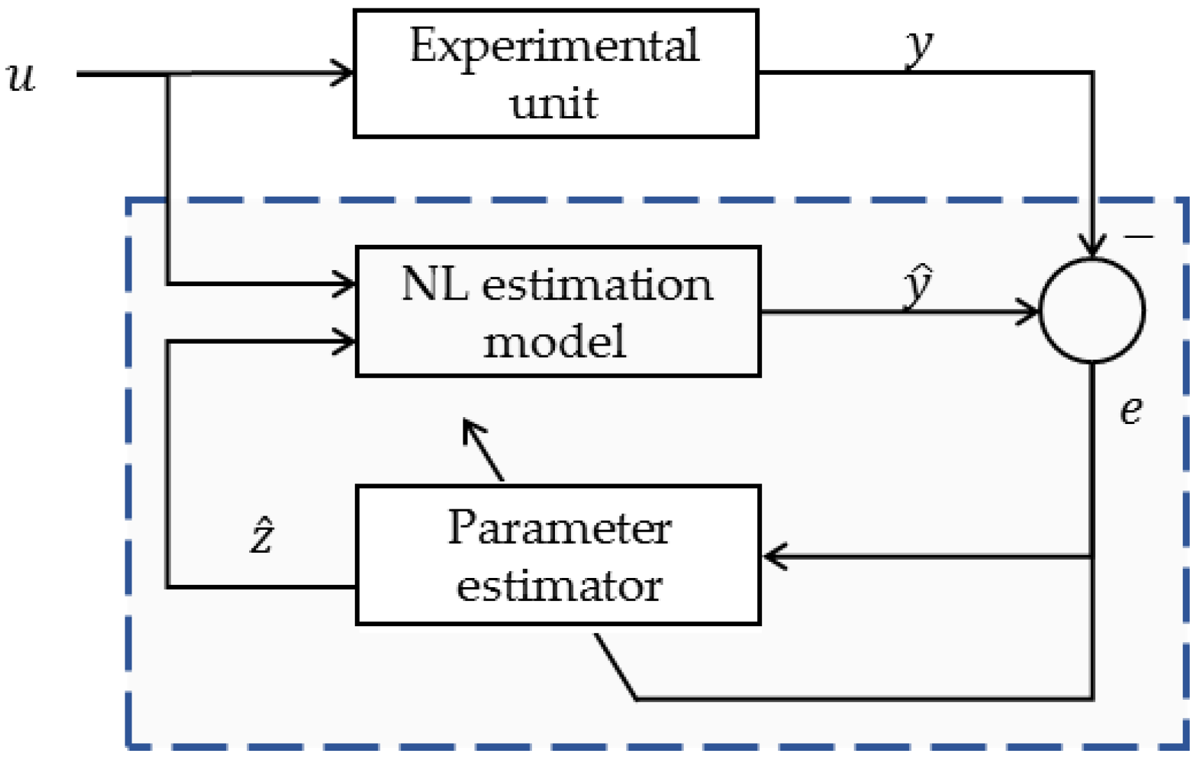
4.2.1. Estimation Problem

The polymerization model described in Equations (8)–(21) can be written in compact discrete-time form as portrayed in Equation (41).

$$\{\begin{array}{c}{\mathit{x}}_{i+1}=f\left({\mathit{x}}_i,{\mathit{u}}_i,\mathit{z}\right)+{\mathit{v}}_i\\ {\mathit{y}}_i=h\left({\mathit{x}}_i,{\mathit{u}}_i,\mathit{z}\right)+{\mathit{w}}_i\end{array}$$

(41)

where $\mathit{x} ϵ {ℝ}^{l_x}$ is the state vector, $\mathit{u} ϵ {ℝ}^{l_u}$ is the vector of inputs, $\mathit{z} ϵ {ℝ}^{l_{\mu }}$ is the unknown parameter vector, $\mathit{y} ϵ {ℝ}^{l_y}$ is the vector of measurements, and $\mathit{v} ϵ {ℝ}^{l_x}$ and $\mathit{w} ϵ {ℝ}^{l_y}$ are the model and measurement errors, respectively.

For estimation purposes, the compact model is considered to be as shown in Equation (42).

$$\{\begin{array}{c}{\widehat{\mathit{x}}}_{i+1}=f\left({\widehat{\mathit{x}}}_i,{\mathit{u}}_i,\widehat{\mathit{z}}\right)+{\mathit{v}}_i\\ {\widehat{\mathit{y}}}_i=h\left({\widehat{\mathit{x}}}_i,{\mathit{u}}_i,\widehat{\mathit{z}}\right)+{\mathit{w}}_i\end{array}$$

(42)

where $\widehat{\mathit{x}}$ is the estimated state vector, $\widehat{\mathit{y}}$ is the vector of estimated measurements, and $\widehat{\mathit{z}}$ is the output of the parameter estimator. The parameter estimator is updated by minimizing a cost function based on the performance variable ($\mathit{e}$).

Considering an ARMA model with a built-in integrator, $\widehat{\mathit{z}}$ is given by:

$${\widehat{\mathit{z}}}_i={\displaystyle \sum }_{l=1}^{n_c}{\mathit{P}}_l{}_i{\widehat{\mathit{z}}}_{i-1}+{\displaystyle \sum }_{l=1}^{n_c}{\mathit{Q}}_l{}_i{\mathit{e}}_{i-l}+{\mathit{R}}_i{\mathit{g}}_i$$

(43)

where,

$${\mathit{g}}_i={\mathit{g}}_{i-1}+{\mathit{e}}_{i-1}$$

(44a)

$${\mathit{e}}_i={\widehat{\mathit{y}}}_i-{\mathit{y}}_i$$

(44b)

and ${\mathit{P}}_i ϵ {ℝ}^{l_z\times l_z}$, ${\mathit{Q}}_i,\mathit{R} ϵ {ℝ}^{l_z\times l_y}$ are the coefficient matrices that are updated recursively by the algorithm. The integrator is combined with the estimator to guarantee that the performance variable approaches to zero as the iterations approach to infinity. Rewriting Equation (43), the following is obtained:

$${\widehat{\mathit{z}}}_i={\Phi }_i{\mathsf{\theta }}_i$$

(45)

where,

$${\mathsf{\Phi }}_i=I_{l_z}\otimes {\mathbf{\varphi }}_i{}^T ϵ {ℝ}^{l_z\times l_{\theta }},$$

(46a)

$${\mathit{\varphi }}_i={\left[{\widehat{\mathit{z}}}_{i-1}{}^T\dots {\widehat{\mathit{z}}}_{i-n_c}{}^T {\mathit{e}}_{i-1}{}^T\dots {\mathit{e}}_{i-n_c}{}^T {\mathit{g}}_i{}^T\right]}^T$$

(46b)

$${\mathsf{\theta }}_i=vec\left[{\mathit{P}}_1{}_i\dots {\mathit{P}}_{n_c}{}_i {\mathit{Q}}_1{}_i\dots {\mathit{Q}}_{n_c}{}_i {\mathit{R}}_i\right] ϵ {ℝ}^{l_{\theta }}$$

(46c)

$$l_{\theta }=l_z{}^2{n}_c+l_z{l}_y\left(n_c+1\right)$$

(46d)

and $\mathsf{\Phi }$ is the regressor matrix, $\mathsf{\theta }$ contains the estimator coefficients computed by the RCMR algorithm. The operator “$⨂$” is the Kronecker product, and $vec$ represents the column-stacking operator.

It is assumed that $\mathit{z}$ is identifiable, which is guaranteed from the global sensitivity analysis (in the absence of an observability/detectability analysis), and that the input signal ${\mathit{u}}_k$ is persistently exciting.

4.2.2. Retrospective Cost Model Refinement (RCMR) Algorithm

The retrospective performance variable is defined as follows:

$${\widehat{\mathit{e}}}_i={\mathit{e}}_i-{\mathit{G}}_f\left(q\right)\left({\Phi }_i\widehat{\mathsf{\theta }}-{\widehat{\mathit{z}}}_i\right)$$

(47)

where $q$ is the forward-shift operator, and $\widehat{\mathsf{\theta }}$ has the parameter estimation coefficients to be optimized.

$${\mathit{G}}_f\left(q\right)={\displaystyle \sum }_{n=1}^{n_f}\frac{{\mathit{N}}_n}{q^n}$$

(48)

For all $n$, ${\mathit{N}}_n ϵ {ℝ}^{l_y\times l_z}$. ${\mathit{G}}_f$ is a finite impulse response filter of order $n_f$. Equation (47) is then rewritten as follows:

$${\widehat{\mathit{e}}}_i={\mathit{e}}_i+\mathit{N}{\Phi }_b{}_i\widehat{\mathsf{\theta }}-\mathit{N}{Z}_b{}_i$$

(49)

where,

$$\mathit{N}=\left[{\mathit{N}}_1\dots {\mathit{N}}_{n_f}\right] ϵ {ℝ}^{l_y\times l_z{n}_f},$$

$${\Phi }_b{}_i=\left[\begin{array}{c}{\mathit{\varphi }}_{i-1}\\ ⋮\\ {\mathit{\varphi }}_{i-n_f}\end{array}\right] ϵ {ℝ}^{l_z{n}_f\times l_{\theta }},$$

$$Z_b{}_i=\left[\begin{array}{c}{\widehat{\mathit{z}}}_{i-1}\\ ⋮\\ {\widehat{\mathit{z}}}_{i-n_f}\end{array}\right] ϵ {ℝ}^{l_z{n}_f}.$$

The retrospective cost function, defined by Goel and Bernstein (2018) [34,35], is minimized by making use of recursive least squares. Let $P_0=R_{\mathsf{\theta }}{}^{-1}$ and ${\mathsf{\theta }}_i=0$.

The algorithm that updates the estimator coefficients is as follows:

$${\mathsf{\theta }}_i={\mathsf{\theta }}_{i-1}-P_i{\Phi }_b{{}_{i-1}}^{\mathrm{T}}{\mathit{N}}^{\mathrm{T}}{R}_{\mathrm{e}}{}_{i-1}\left(\mathrm{N}{\Phi }_b{}_{i-1}{\mathsf{\theta }}_{i-1}+{\mathit{e}}_{i-1}-\mathit{N}{Z}_b{}_{i-1}\right)$$

(50)

$$P_i={\mathsf{\lambda }}^{-1}{P}_{i-1}-{\mathsf{\lambda }}^{-1}{P}_{i-1}{\Phi }_b{{}_{i-1}}^T{\mathit{N}}^{\mathrm{T}}{\mathsf{\Gamma }}_i{}^{-1}\mathit{N}{\Phi }_b{}_{i-1}{P}_{i-1}$$

(51)

$${\mathsf{\Gamma }}_i=\mathsf{\lambda }{R}_{\mathrm{e}}{{}_{i-1}}^{-1}+\mathit{N}{\Phi }_b{}_{i-1}{P}_{i-1}{\Phi }_b{{}_{i-1}}^T{\mathit{N}}^{\mathrm{T}}$$

(52)

where $R_{\mathrm{e}}$ and $R_{\mathsf{\theta }}$ are positive-definite matrices, and $\mathsf{\lambda }\le 1$ is the forgetting factor.

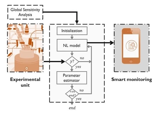
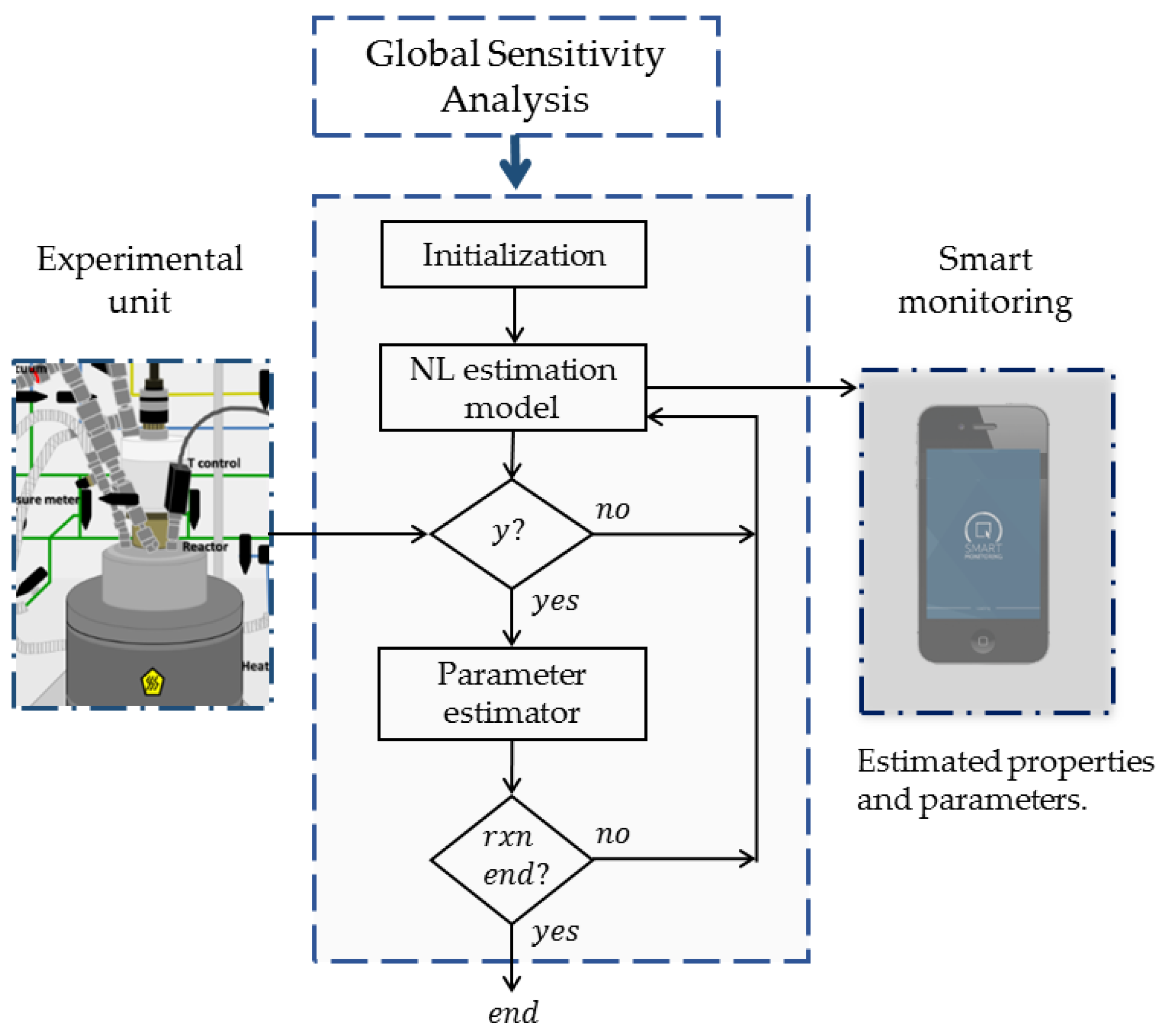
4.3. Framework Implementation

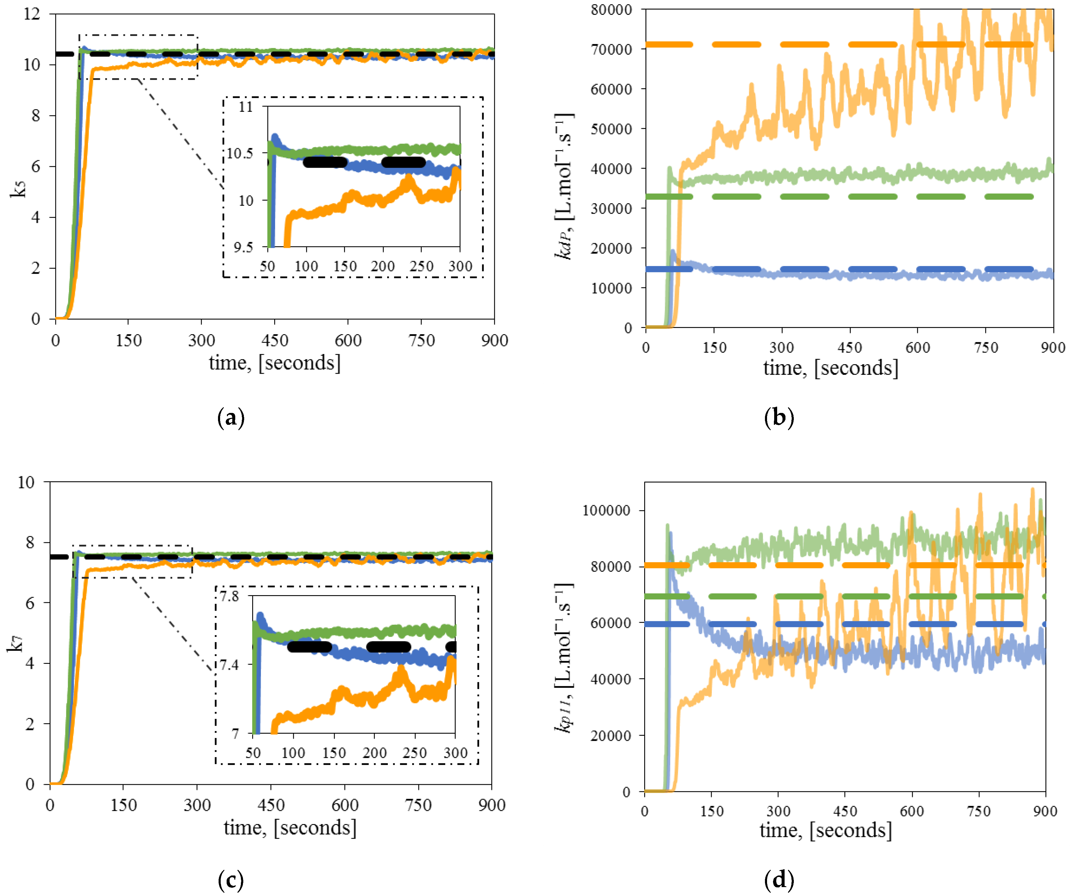
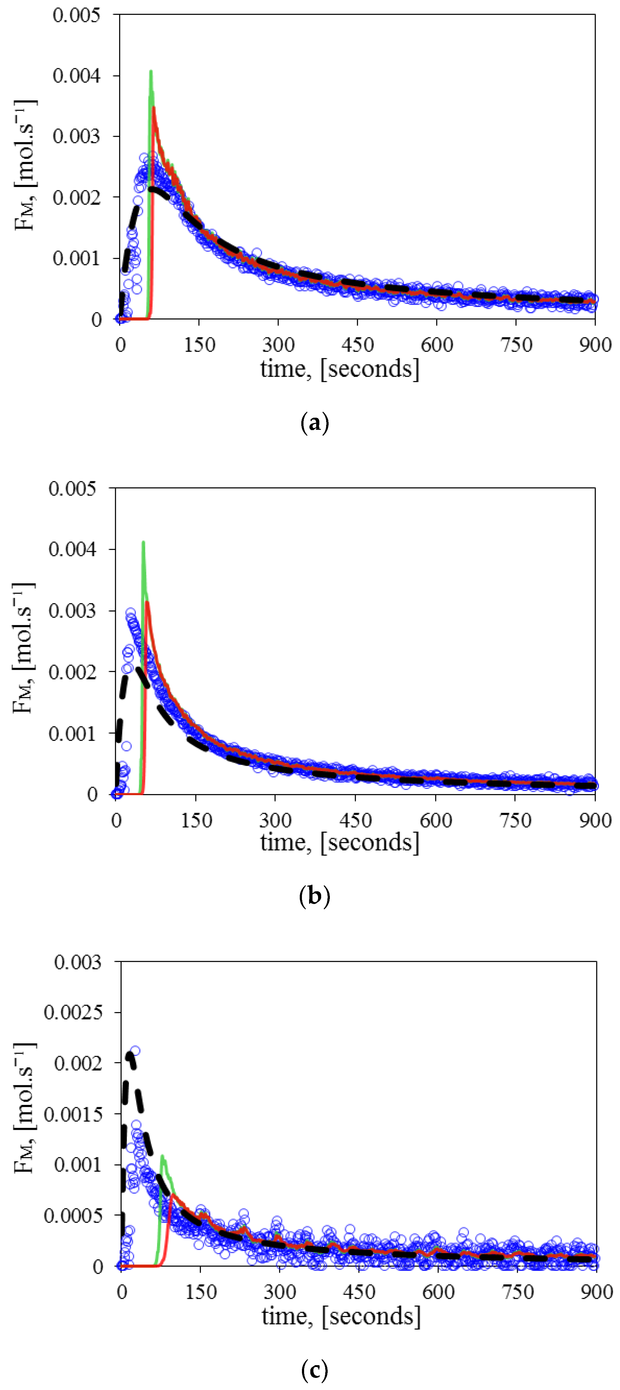
The assembly of the implemented strategies is summarized in Figure 1. Initially, the global sensitivity analysis provides information on the most important parameters of the polymerization system. Once these parameters are identified, the proposed framework tries to estimate their values asynchronously, updating/estimating the parameters whenever measurements are available. Monitoring and signal processing are other challenges of the proposed methodology. The estimated properties are expected to be close to the experimental and theoretical values, and noise reduction of the measurements is anticipated to occur.

Figure 2 portrays the architecture of the data-driven estimation strategy. The experimental unit generates measurements $\mathit{y}$, which are assumed to be driven by the inputs $\mathit{u}$. The data-driven adaptive estimator consists of the nonlinear estimation model, which is also driven by the inputs $\mathit{u}$, and the RCMR algorithm. Although the nonlinear estimation model is required to generate the estimated measurements $\widehat{\mathit{y}}$, it does not provide knowledge for the parameter updates. The estimated parameter $\widehat{\mathit{z}}$ is updated by the estimator, which seeks the minimization of the error signal $\mathit{e}$.

5. Results

$F_{\mathrm{M}}$ is the only measurement obtained continuously. Thus, the global sensitivity analysis and the data-driven estimation are performed using $F_{\mathrm{M}}$ as the input signal. The other available measurements ($M_{\mathrm{w}}, M_{\mathrm{n}}$) are employed as a reference for comparing the accuracy of the estimated properties.

The system was simulated in MATLAB R2015a, running on a PC Intel Core™ i7-4790K CPU @ 4.00 GHz with 16.0 Gb of installed RAM. The ODEs of the system were solved using ode23s [43], based on a modified Rosenbrock formula of order 2. The sampling time of $F_{\mathrm{M}}$ was every 1 s, and the RCMR algorithm together with the nonlinear model run in approximately 0.0035 s, which makes feasible the online deployment of the proposed strategy. Computational methods can be used for online applications if they are faster than the real process by a factor of 100 [44].

5.1. Global Sensitivity Analysis

From the global sensitivity analysis of the seven kinetic parameters ($k_{1-7}$), the fifth and seventh show the highest overall sensitivity, as portrayed in Figure 3. This result is consistent because $k_7$ is the exponent in the pre-exponential propagation rate constant ($k_0{}_p={10}^{k_7}$) of the Arrhenius equation. The propagation rate constant determines the monomer consumption rate; thus, it strongly influences the value of $F_{\mathrm{M}}$ (ethylene flow rate to the reactor), seeking to maintain the ethylene concentration in the reactor constant during the polymerization. The rate constant for the living chain (catalyst) deactivation ($k_{dP}$) is a function of $k_5$ (as defined in Table 1). Since $k_{dP}$ influences the moment equations, it is expected that this parameter is influential as well. These results are in agreement with the work of Brandão et al. (2017) [13], because $k_5$ and $k_7$ belong to the parameter set classified as significant when an identifiability analysis was applied over the seven parameters. Figure 3a illustrates the first-order, and Figure 3b the total sensitivity indices when using 100 samples.

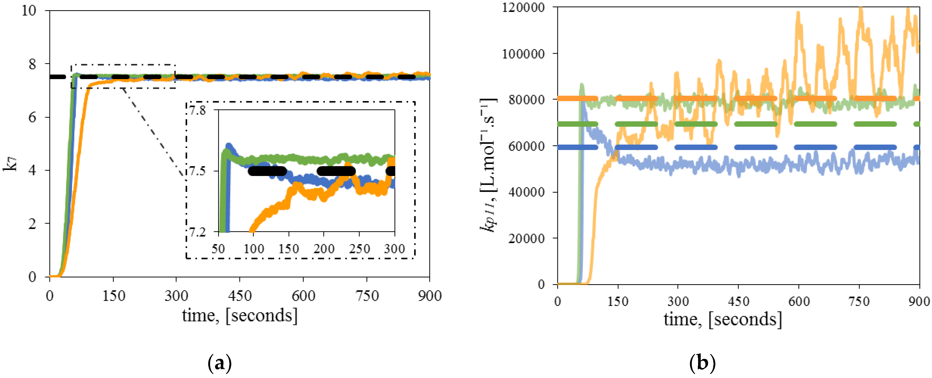
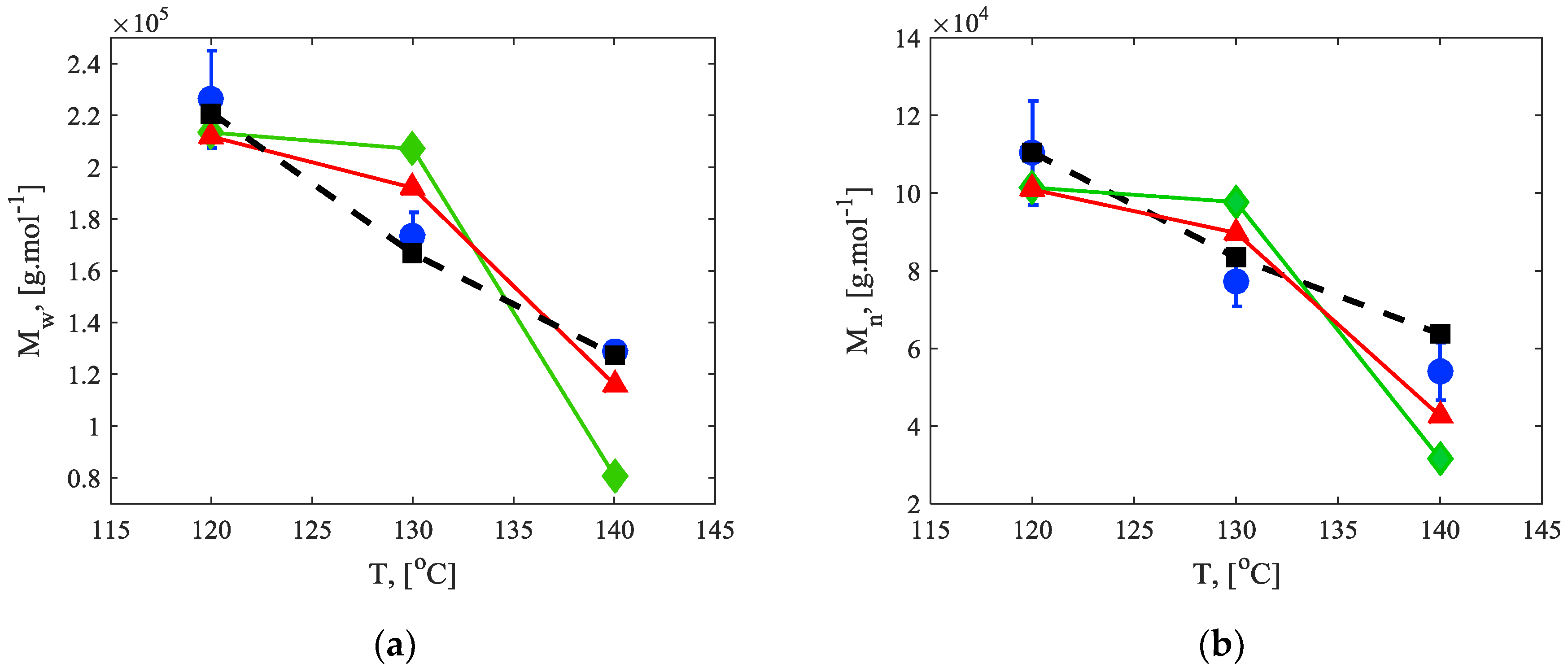
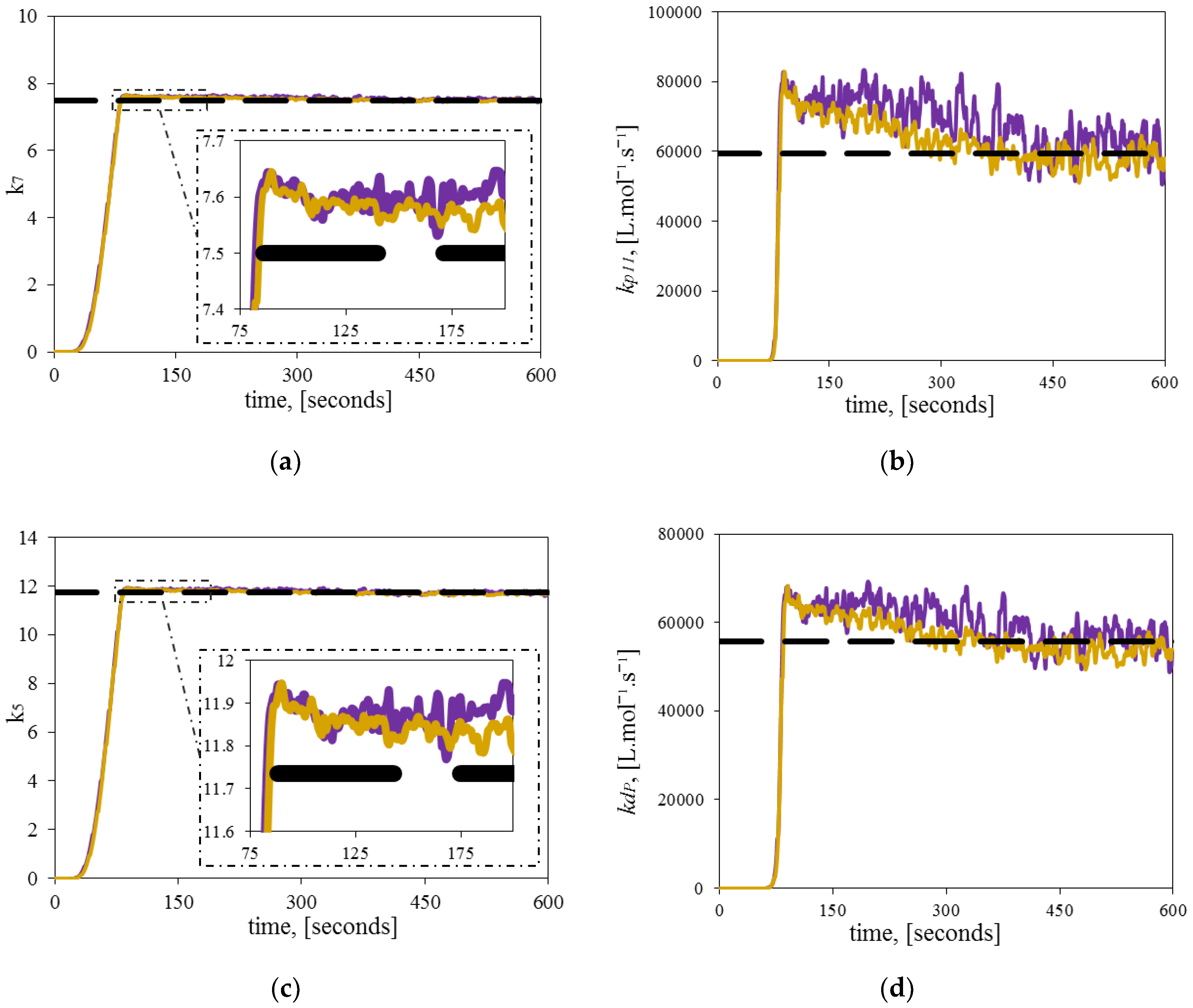
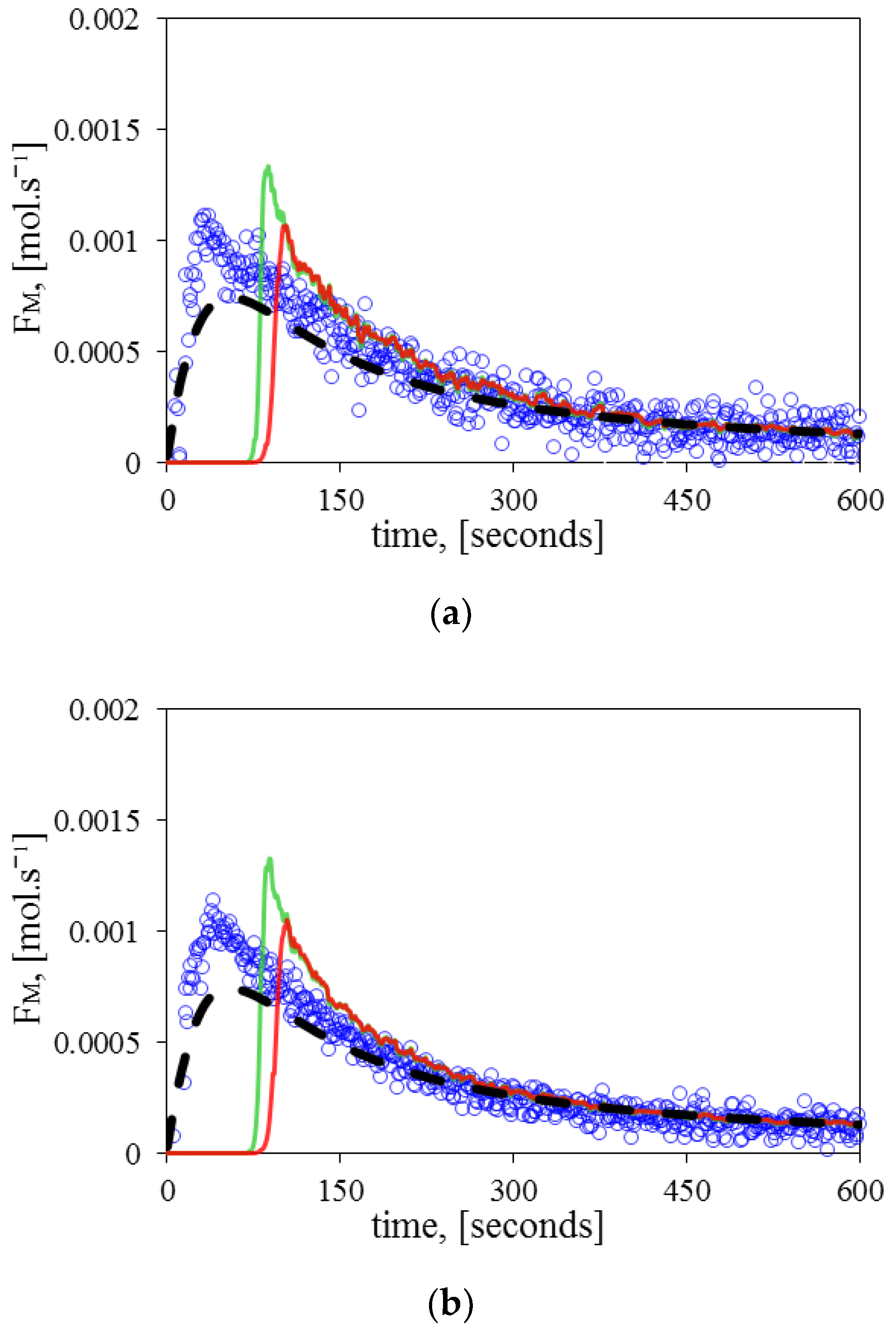
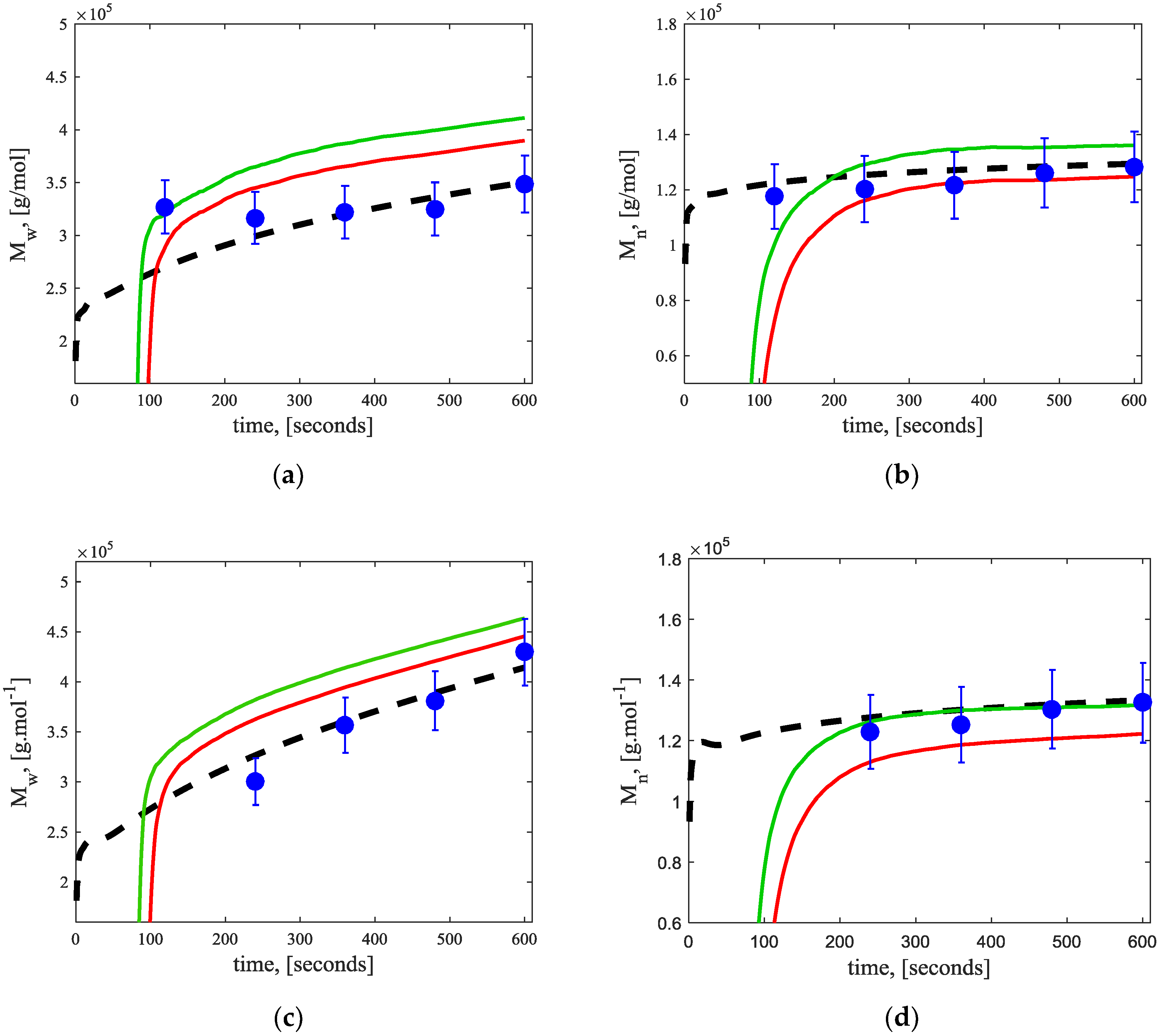
5.2. Homopolymerization

Homopolymerization experiments at different reaction temperatures were used to test the RCMR algorithm on its kinetic parameter estimation capabilities. The RCMR algorithm was implemented considering: $P_0=R_{\mathsf{\theta }}{}^{-1}$, ${\mathsf{\theta }}_0=0$, and $n_c=0$.

Initially, only $k_7$, and consequently $k_{{\mathrm{p}}_{11}}$, were estimated, using the initial guess $k_7$ = 0. To improve the convergence of the algorithm it was assumed that $l_z=2$, meaning that two parameters were estimated rather than one. For the non-estimated parameter, a constant value of $\widehat{z}=11.3$ provided a satisfactory response and tradeoff. With these considerations, the architecture selected was: $n_f=2$ so that $l_{\theta }=2$, $\mathsf{\lambda }=0.999$, and

$${\mathit{G}}_f\left(q\right)=\frac{\left[\begin{array}{cc}1& 0\end{array}\right]}{q}+\frac{\left[\begin{array}{cc}0& 1\end{array}\right]}{q^2}$$

(53)

For estimating a single parameter, the algorithm considered $R_{\theta }=0.01{\mathit{I}}_{l_{\mathsf{\theta }}}$, and $R_{\mathrm{e}}=0.1$.

Figure 4 shows the estimates for $k_7$ and $k_{{\mathrm{p}}_{11}}$ at different polymerization temperatures. The estimated parameters converge, in all cases, close to theoretical values without requiring prior knowledge of the initial value or range of the parameter.

Furthermore, the most significant kinetic parameters of the system, $k_5$ and $k_7$, and consequently $k_{dP}$ and $k_{{\mathrm{p}}_{11}}$, were estimated simultaneously. The same architecture implemented for single parameter estimation was used in the simultaneous estimation, with the distinction that the parameters were estimated in separate channels using the same error signal. The non-estimated parameters were different: ${\widehat{z}}_{k_5}=23.5$, and ${\widehat{z}}_{k_7}=15.0$, and everything else remained the same.

Figure 5 shows the results of the estimated $k_5$, $k_{dP}$, $k_7$, and $k_{{\mathrm{p}}_{11}}$ at different polymerization temperatures. In all cases, the estimated parameters ($k_5$, $k_7$) approached their theoretical values, converging from an initial value of 0 in both cases. A noisy response was observed, as in Figure 4, which can be attributed to the presence of impurities that could not be removed during the experiments, or to the occurrence of side reactions not included in the fundamental model. In addition, as the polymerization temperature increased, the estimated parameters became more sensitive to noise, which provided the insight that temperature is proportional to the noise/uncertainty of the experimental data.

Figure 6 illustrates how the RCMR can both estimate $F_{\mathrm{M}}$ and reduce the measurement’s noise. The reader should note that it takes some time for the estimated $F_{\mathrm{M}}$ to achieve its expected value. Goel and Bernstein (2018) [13] explained that the unknown parameter moves towards different subspaces until it tends to the subspace spanned by ${\mathit{N}}_1{}^T$. In addition, there is a delay time difference between the estimated ${\widehat{F}}_{\mathrm{M}}$ with a single and two parameters, which is mostly related to the tuning. Finally, as stated before, the ${\widehat{F}}_{\mathrm{M}}$ at the highest temperature (140 °C) shows an oscillatory response.

Figure 7 compares the results computed by the nonlinear model, the measured results, and the estimated average properties at different polymerization temperatures. The results at 120 °C of both $M_{\mathrm{w}}$ and $M_{\mathrm{n}}$ are very close to their theoretical and experimental values, but as the temperature increases, the uncertainty also increases. The estimation of two parameters simultaneously appears to provoke less reliable results when compared to the estimated properties with a single parameter, especially at higher temperatures.

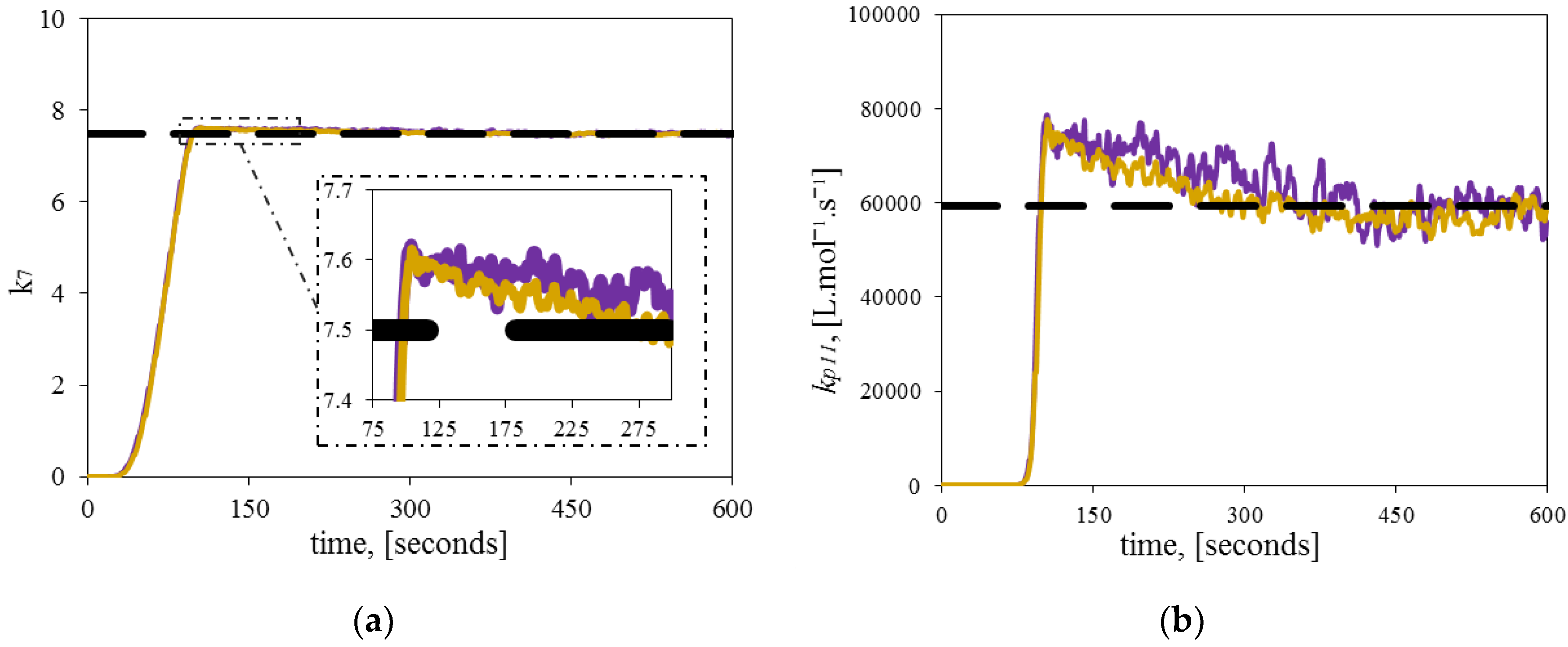
5.3. Copolymerization

Following the criterion used for the homopolymerization experiments, the copolymerizations used the same RCMR architecture for the estimation of significant kinetic parameters and important polymer properties. Indeed, the criterion extends to the application of the same channels for estimating one and two significant kinetic parameters and their resulting properties.

The copolymerization experiments considered only one temperature. Initially, $k_7$ and consequently $k_{{\mathrm{p}}_{11}}$ were estimated for the copolymerizations described in Table 4a,b. Figure 8 illustrates the results of the estimated $k_7$ and $k_{{\mathrm{p}}_{11}}$ at 120 °C and different initial diene concentrations. The unknown parameter converges towards the theoretical value without requiring prior knowledge at both initial diene concentrations.

Moreover, the parameters $k_5$ and $k_7$, and, consequently, $k_{dP}$ and $k_{{\mathrm{p}}_{11}}$, were estimated simultaneously, using the same architecture and tuning used in the homopolymerizations. Figure 9 shows the results of the estimated $k_5$, $k_{dP}$, $k_7$, and $k_{{\mathrm{p}}_{11}}$ at different initial diene concentrations at 120 °C. In all cases, the unknown parameters $k_5$ and $k_7$ approach the theoretical values, starting from an initial guess of 0. An interesting observation in these experiments is the slight decreasing trend (negative slope) of the parameters, made clearer in the dynamic evolution of $k_{dP}$ and $k_{{\mathrm{p}}_{11}}$. The reason for this behavior might be related to LCBs formation during the copolymerization. The presence of LCBs in the living chains might cause a steric hindrance to the incorporation of ethylene molecules, which disfavors deactivation and propagation reactions. However, this hypothesis must be proved by additional experiments and further simulations.

Figure 10 demonstrates how the RCMR can estimate $F_{\mathrm{M}}$ effectively and reduce the measurement’s noise. As before, it takes some time for the estimated $F_{\mathrm{M}}$ to achieve values close to experimental and theoretical values. There are no visible differences observed when the initial concentration of diene varies, which makes it possible to conclude that temperature is more influential on the reaction behavior. In contrast to the homopolymerization results (Figure 6), the estimated $F_{\mathrm{M}}$ in the copolymerization experiments shows a higher delay time of convergence. It could be argued that it should be influenced by the increase in the complexity of modelling, but because the RCMR algorithm is a purely data-driven strategy, which does not require information on the nonlinear model, the reasons must be totally related to the nature of the experiment.

Finally, Figure 11 compares the results computed by the fundamental model, the measured results, and the estimated average properties of the copolymerization experiments at different initial diene concentrations. Data on the average properties was obtained during the polymerization experiments. The results show that the RCMR algorithm, besides computing the unknown parameters, can estimate $M_{\mathrm{n}}$ satisfactorily using the error signal obtained as the difference between the estimated and measured $F_{\mathrm{M}}$. This signal allows the estimator to gain enough information on the system to estimate $M_{\mathrm{n}}$. Of course, the estimation additionally relies on the correctness of the model and the non-estimated parameters as well, but the obtained results are comparable with theoretical and experimental values. On the other hand, $M_{\mathrm{w}}$ achieves a similar dynamic when compared to the fundamental model, but the estimates fail to attain perfect values close to the experimental measurements.

6. Conclusions

In this contribution, a data-driven strategy for the online estimation of important kinetic parameters was assessed and implemented for the copolymerization of ethylene with 1,9-decadiene using dimethylsilyl (N-tert-butylamido) (tetramethylcyclopentadienyl) titanium dichloride (CGC)/MAO as catalyst. A global sensitivity analysis was performed initially to all polymerization kinetic parameters. The first and total sensitivity indices made it possible to choose the significant parameters of the model. Thereafter, the RCMR algorithm, a strategy never implemented in polymerization applications, permitted the estimation of the significant kinetic parameters, which were assumed to be unknown. After verifying consistency, the proposed strategy was tested in the copolymerization of ethylene with 1,9-decadiene at different diene concentrations. Overall, results were satisfactory, showing not only adequacy in signal processing, but also in parameter and property estimation.

The usage of data-driven algorithms such as the RCMR represents a paradigm that could permit easier estimation of parameters of nonlinear systems, such as those observed in polymer synthesis. Disturbances in the experimental data (e.g., impurities, experimental errors, and less frequent side reactions) that might not be captured by the fundamental model could be overcome by applying this strategy.

The proposed strategy also holds the advantage that it is capable of being adapted to the conditions of the experiment, and it can estimate the important kinetic parameters of the system while the reaction is running. This could be beneficial for processes where the major kinetic parameters are unknown for all the different types of catalysts, or the composition of the catalysts might be slightly different from each other, resulting in important differences. In the particular case of the RCMR algorithm, it has the additional advantage of estimating the parameters from an initial value of zero without requiring knowledge of the model.

Future work in this field will include the evaluation of the proposed framework and estimation algorithm in other chemical processes and polymerization systems.

References

1. Liu, P.; Liu, W.; Wang, W.J.; Li, B.G.; Zhu, S. A Comprehensive Review on Controlled Synthesis of Long-Chain Branched Polyolefins: Part 1, Single Catalyst Systems. Macromol. React. Eng. 2016, 10, 156–179. [Google Scholar] [CrossRef] [Green Version]
2. Stadler, F.J.; Piel, C.; Klimke, K.; Kaschta, J.; Parkinson, M.; Wilhelm, M.; Münstedt, H. Influence of type and content of various comonomers on long-chain branching of ethene/α-olefin copolymers. Macromolecules 2006, 39, 1474–1482. [Google Scholar] [CrossRef]
3. Soares, J.B.; Hamielec, A.E. Bivariate chain length and long chain branching distribution for copolymerization of olefins and polyolefin chains containing terminal double-bonds. Macromol. Theory Simul. 1996, 5, 547–572. [Google Scholar] [CrossRef]
4. Wang, W.J.; Yan, D.; Zhu, S.; Hamielec, A.E. Kinetics of long chain branching in continuous solution polymerization of ethylene using constrained geometry metallocene. Macromolecules 1998, 31, 8677–8683. [Google Scholar] [CrossRef]
5. Chum, P.S.; Kruper, W.J.; Guest, M.J. Materials properties derived from INSITE metallocene catalysts. Adv. Mater. 2000, 12, 1759–1767. [Google Scholar] [CrossRef]
6. Choo, T.N.; Waymouth, R.M. Cyclocopolymerization: A mechanistic probe for dual-site alternating copolymerization of ethylene and α-olefins. J. Am. Chem. Soc. 2002, 124, 4188–4189. [Google Scholar] [CrossRef]
7. Naga, N.; Toyota, A. Unique Insertion Mode of 1,7-Octadiene in Copolymerization with Ethylene by a Constrained-Geometry Catalyst. Macromol. Rapid Commun. 2004, 25, 1623–1627. [Google Scholar] [CrossRef]
8. Mehdiabadi, S.; Soares, J.B. Production of Ethylene/α-Olefin/1, 9-Decadiene Copolymers with Complex Microstructures Using a Two-Stage Polymerization Process. Macromolecules 2011, 44, 7926–7939. [Google Scholar] [CrossRef]
9. Soares, J.B. Mathematical Modeling of the Long-Chain Branch Structure of Polyolefins Made with Two Metallocene Catalysts: An Algebraic Solution. Macromol. Theory Simul. 2002, 11, 184–198. [Google Scholar] [CrossRef]
10. Ferreira, L.C., Jr.; Nele, M.; Costa, M.A.; Pinto, J.C. Mathematical Modeling of MWD and CBD in Polymerizations with Macromonomer Reincorporation and Chain Running. Macromol. Theory Simul. 2010, 19, 496–513. [Google Scholar] [CrossRef]
11. Mogilicharla, A.; Mitra, K.; Majumdar, S. Modeling of propylene polymerization with long chain branching. Chem. Eng. J. 2014, 246, 175–183. [Google Scholar] [CrossRef]
12. Albeladi, A.; Mehdiabadi, S.; Soares, J.B. Modeling Possible Long Chain Branching Reactions for Polyethylene in a Semi-Batch Reactor. 2018. Available online: http://dc.engconfintl.org/prex/49 (accessed on 26 February 2019).
13. Brandão, A.L.; Alberton, A.L.; Pinto, J.C.; Soares, J.B. Copolymerization of Ethylene with 1, 9-Decadiene: Part I–Prediction of Average Molecular Weights and Long-Chain Branching Frequencies. Macromol. Theory Simul. 2017, 26, 1600059. [Google Scholar] [CrossRef]
14. Brandão, A.L.; Alberton, A.L.; Pinto, J.C.; Soares, J.B. Copolymerization of Ethylene with 1, 9-Decadiene: Part II—Prediction of Molecular Weight Distributions. Macromol. Theory Simul. 2017, 26, 1700040. [Google Scholar] [CrossRef]
15. Soares, J.B.; McKenna, T.F. Polyolefin Reaction Engineering; John Wiley & Sons: Hoboken, NJ, USA, 2013. [Google Scholar]
16. Qin, S.J. Process data analytics in the era of big data. AIChE J. 2014, 60, 3092–3100. [Google Scholar] [CrossRef]
17. Salas, S.D.; Ghadipasha, N.; Zhu, W.; Mcafee, T.; Zekoski, T.; Reed, W.F.; Romagnoli, J.A. Framework Design for Weight-Average Molecular Weight Control in Semi-Batch Polymerization. Control Eng. Pract. 2018, 78, 12–23. [Google Scholar] [CrossRef]
18. Kozub, D.J.; MacGregor, J.F. State estimation for semi-batch polymerization reactors. Chem. Eng. Sci. 1992, 47, 1047–1062. [Google Scholar] [CrossRef]
19. Tatiraju, S.; Soroush, M. Nonlinear state estimation in a polymerization reactor. Ind. Eng. Chem. Res. 1997, 36, 2679–2690. [Google Scholar] [CrossRef]
20. Lopez, T.; Alvarez, J. On the effect of the estimation structure in the functioning of a nonlinear copolymer reactor estimator. J. Process Control 2004, 14, 99–109. [Google Scholar] [CrossRef]
21. Galdeano, R.; Asteasuain, M.; Sánchez, M.C. Unscented transformation-based filters: Performance comparison analysis for the state estimation in polymerization processes with delayed measurements. Macromol. React. Eng. 2011, 5, 278–293. [Google Scholar] [CrossRef]
22. Hashemi, R.; Kohlmann, D.; Engell, S. Optimizing control and state estimation of a continuous polymerization process in a tubular reactor with multiple side-streams. Macromol. React. Eng. 2016, 10, 415–434. [Google Scholar] [CrossRef]
23. Zoellner, K.; Reichert, K.H. Gas phase polymerization of butadiene—Kinetics, particle size distribution, modeling. Chem. Eng. Sci. 2001, 56, 4099–4106. [Google Scholar] [CrossRef]
24. Ghadipasha, N.; Geraili, A.; Romagnoli, J.A.; Castor, C.A.; Drenski, M.F.; Reed, W.F. Combining on-line characterization tools with modern software environments for optimal operation of polymerization processes. Processes 2016, 4, 5. [Google Scholar] [CrossRef]
25. Schwaab, M.; Biscaia, E.C., Jr.; Monteiro, J.L.; Pinto, J.C. Nonlinear parameter estimation through particle swarm optimization. Chem. Eng. Sci. 2008, 63, 1542–1552. [Google Scholar] [CrossRef]
26. Salas, S.D.; Romagnoli, J.A.; Tronci, S.; Baratti, R. A geometric observer design for a semi-batch free-radical polymerization system. Comput. Chem. Eng. 2019, 126, 391–402. [Google Scholar] [CrossRef]
27. Sirohi, A.; Choi, K.Y. On-line parameter estimation in a continuous polymerization process. Ind. Eng. Chem. Res. 1996, 35, 1332–1343. [Google Scholar] [CrossRef]
28. Li, R.; Corripio, A.B.; Henson, M.A.; Kurtz, M.J. On-line state and parameter estimation of EPDM polymerization reactors using a hierarchical extended Kalman filter. J. Process Control 2004, 14, 837–852. [Google Scholar] [CrossRef]
29. Chen, T.; Morris, J.; Martin, E. Particle filters for state and parameter estimation in batch processes. J. Process Control 2005, 15, 665–673. [Google Scholar] [CrossRef] [Green Version]
30. Sheibat-Othman, N.; Peycelon, D.; Othman, S.; Suau, J.M.; Fevotte, G. Nonlinear observers for parameter estimation in a solution polymerization process using infrared spectroscopy. Chem. Eng. J. 2008, 140, 529–538. [Google Scholar] [CrossRef]
31. Salas Ortiz, S.D. A Model-Based Framework for the Smart Manufacturing of Polymers. Ph.D. Thesis, Louisiana State University and Agricultural and Mechanical College, Baton Rouge, LA, USA, 2019; p. 4897. [Google Scholar]
32. Wu, Q.L.; Cournede, P.H.; Mathieu, A. An efficient computational method for global sensitivity analysis and its application to tree growth modelling. Reliab. Eng. Syst. Saf. 2012, 107, 35–43. [Google Scholar] [CrossRef]
33. Goel, A.; Duraisamy, K.; Bernstein, D.S. Parameter estimation in the burgers equation using retrospective-cost model refinement. In Proceedings of the American Control Conference (ACC), Boston, MA, USA, 6–8 July 2016; pp. 6983–6988. [Google Scholar]
34. Goel, A.; Bernstein, D.S. Parameter estimation for nonlinearly parameterized gray-box models. In Proceedings of the Annual American Control Conference (ACC), Milwaukee, WI, USA, 27–29 June 2018; pp. 5280–5285. [Google Scholar]
35. Goel, A.; Bernstein, D.S. Data-Driven Parameter Estimation for Models with Nonlinear Parameter Dependence. In Proceedings of the 2018 IEEE Conference on Decision and Control (CDC), Miami Beach, FL, USA, 17–19 December 2018; pp. 1470–1475. [Google Scholar]
36. Hulburt, H.M.; Katz, S. Some problems in particle technology: A statistical mechanical formulation. Chem. Eng. Sci. 1964, 19, 555–574. [Google Scholar] [CrossRef]
37. Eberhart, R.; Kennedy, J. Particle Swarm Optimization. In Proceedings of the IEEE International Conference on Neural Networks, Perth, Australia, 27 November–1 December 1995; pp. 1942–1948. [Google Scholar]
38. Sobol, I.M. Sensitivity estimates for nonlinear mathematical models. Math. Model. Comput. Exp. 1993, 1, 407–414. [Google Scholar]
39. Cosenza, A.; Mannina, G.; Vanrolleghem, P.A.; Neumann, M.B. Variance-based sensitivity analysis for wastewater treatment plant modelling. Sci. Total Environ. 2014, 470, 1068–1077. [Google Scholar] [CrossRef]
40. Saltelli, A. Making best use of model evaluations to compute sensitivity indices. Comput. Phys. Commun. 2002, 145, 280–297. [Google Scholar] [CrossRef]
41. Saltelli, A.; Ratto, M.; Andres, T.; Campolongo, F.; Cariboni, J.; Gatelli, D.; Tarantola, S. Global Sensitivity Analysis: The Primer; John Wiley & Sons: Hoboken, NJ, USA, 2008. [Google Scholar]
42. Salas, S.D.; Geraili, A.; Romagnoli, J.A. Optimization of Renewable Energy Businesses under Operational Level Uncertainties through Extensive Sensitivity Analysis and Stochastic Global Optimization. Ind. Eng. Chem. Res. 2017, 56, 3360–3372. [Google Scholar] [CrossRef]
43. Shampine, L.F.; Reichelt, M.W. The matlab ode suite. SIAM J. Sci. Comput. 1997, 18, 1–22. [Google Scholar] [CrossRef]
44. Porru, M.; Ożkan, L. Monitoring of Batch Industrial Crystallization with Growth, Nucleation, and Agglomeration. Part 2: Structure Design for State Estimation with Secondary Measurements. Ind. Eng. Chem. Res. 2017, 56, 9578–9592. [Google Scholar] [CrossRef] [Green Version]
Figure 1. Framework for the online estimation of significant kinetic parameters.
Processes 07 00309 g001
Figure 2. Data-driven parameter estimation architecture.
Processes 07 00309 g002
Figure 3. Global sensitivity indices: (a) first-order sensitivity index; (b) total sensitivity index.
Processes 07 00309 g003
Figure 4. Estimation of a single significant parameter. Comparison between theoretical (dashed line), and estimated kinetic parameters (continuous line) at 120 °C (blue), 130 °C (green) 140 °C (orange): (a) Dynamic estimation of k 7 ; (b) Dynamic estimation of k p 11 .
Processes 07 00309 g004
Figure 5. Estimation of two significant parameters. Comparison between theoretical (dashed line), and estimated kinetic parameters (continuous line) at 120 °C (blue), 130 °C (green) 140 °C (orange): (a) Dynamic estimation of k 5 ; (b) Dynamic estimation of k d P ; (c) Dynamic estimation of k 7 , (d) Dynamic estimation of k p 11 .
Processes 07 00309 g005
Figure 6. Comparison of the monomer flow rate ( F M ) between the experimental values (circles), fundamental model (dashed line), estimated with a single parameter (continuous red line), and estimated with two parameters (continuous green line) at: (a) 120 °C, (b) 130 °C, (c) 140 °C.
Processes 07 00309 g006
Figure 7. Comparison of the final average properties at different temperatures for experimental values (circles), fundamental model (squares–dashed line), estimated with a single parameter (triangles–continuous line), and estimated with two parameters (diamonds–continuous line): (a) weight-average molecular weight ( M w ); (b) number-average molecular weight ( M n ).
Processes 07 00309 g007
Figure 8. Estimation of a single significant parameter. Comparison between theoretical (dashed line), and estimated kinetic parameters (continuous line) at different initial diene concentrations for the copolymerization experiment A (purple), and copolymerization experiment B (gold); (a) Dynamic estimation of k 7 ; (b) Dynamic estimation of k p 11 .
Processes 07 00309 g008
Figure 9. Estimation of two significant parameters. Comparison between theoretical (dashed line), and estimated kinetic parameters (continuous line) at different initial diene concentrations for the copolymerization experiment A (purple), and copolymerization experiment B (gold): (a) Dynamic estimation of k 7 ; (b) Dynamic estimation of k p 11 ; (c) Dynamic estimation of k 5 ; (d) Dynamic estimation of k d P .
Processes 07 00309 g009
Figure 10. Comparison of the monomer flow rate ( F M ) during copolymerization between the experimental values (circles), fundamental model (dashed line), estimated with a single parameter (continuous red line), and estimated with two parameters (continuous green line) at different initial diene concentrations: (a) copolymerization experiment A, (b) copolymerization experiment B.
Processes 07 00309 g010
Figure 11. Comparison of average polymer properties at different initial diene concentrations between experimental values (circles), fundamental model (dashed line), estimated with a single parameter (red continuous line), and estimated with two parameters (green continuous line). (a) Weight-average molecular weight ( M w ) for copolymerization A; (b) number-average molecular weight ( M n ) for copolymerization A; (c) weight-average molecular weight ( M w ) for copolymerization B; (d) number-average molecular weight ( M n ) for copolymerization B.
Processes 07 00309 g011