Abstract
Non-intrusive load monitoring (NILM) is an effective method to optimize energy consumption patterns. Since the concept of NILM was proposed, extensive research has focused on energy disaggregation or load identification. The traditional method is to disaggregate mixed signals, and then identify the independent load. This paper proposes a multi-label classification method using Random Forest (RF) as a learning algorithm for non-intrusive load identification. Multi-label classification can be used to determine which categories data belong to. This classification can help to identify the operation states of independent loads from mixed signals without disaggregation. The experiments are conducted in real environment and public data set respectively. Several basic electrical features are selected as the classification feature to build the classification model. These features are also compared to select the most suitable features for classification by feature importance parameters. The classification accuracy and F-score of the proposed method can reach 0.97 and 0.98, respectively.
1. Introduction
Load monitoring technology is of great significance to the demand side management (DSM) [1]. It can transfer the collected user’s power consumption information to the grid to improve the efficiency of power grid utilization, and it can help users to adjust their electricity consumption habits [2].
Load monitoring technology contains two categories: “intrusive” and “non-intrusive”. Usually, the intrusive load monitoring needs to place sensors in the users’ internal electric load. In the installation and maintenance process of the sensors, a power cut is needed. Although the data obtained by this technology is reliable, it is not easy for users to accept it. In contrast, non-intrusive load monitoring (NILM) can monitor the whole internal load of the user by placing a monitoring device at the entrance of the user’s power supply, which has little impact on the user. Therefore, this has great potential for development.
Machine learning is an effective method for data processing. It can be used in classification and prediction. Various models are used to predict energy consumption [3]. Model predictive control with machine learning algorithm was used [4]. Madhur provided a model-based control with regression trees algorithm for demand response [5]. In this paper, machine learning was used in NILM, and with the development of AI technology, the cost of AI chip becomes lower. It is possible to use machine learning to process real-time data by placing AI chips in monitoring devices. Therefore, the machine learning method becomes a practical and efficient way to deal with NILM. Load identification is the most important step in NILM, which directly reflects user’s load usage information. Thus, after Hart proposed the concept of NILM [6], a large number of machine learning methods were used for load identification [7]. These machine learning methods can be divided into supervised learning and unsupervised learning. Unsupervised learning does not require labeled data to build models. Hidden Markov Model (HMM) is a typical method of unsupervised learning. Based on a Bayesian treatment of HMM, Parson [8] proposed a hierarchical approach which models multiple appliances of the same type. However, this method requires a lot of data and time to build the model, which is also the common fault of unsupervised learning. In contrast, supervised learning only requires correct input and output data to build a model for new data [9]. Thus, more supervised learning is used in NILM like Support Vector Machines (SVM), k-Nearest Neighbor (k-NN), and clustering methods such as k-means. The k-NN method was applied [10,11,12,13,14,15]. The k-NN method was used to identify five common electrical appliances [10]. Chahine proposed a new feature extraction scheme to build a data set, and then used it to train k-NN [11]. Rahimi used the real power and reactive power as features in k-NN for describing the load-signatures of individual devices, which achieved great accuracy [13]. Figueiredo developed an algorithm [14] which extracted features from active powers, reactive powers and power factor as train data for k-NN. The neural networks were used [16,17,18,19,20]. Chang used wavelet coefficients as features in neural networks [16,17]. Semwal selected the major eight harmonics of load-signatures as features [18]. The Multilayer Perceptron-Artificial Neural Network (MLP-ANN) classifier achieved high accuracy. Srinivasan used current harmonics as a training feature and utilized particle swarm optimization method to train the weights of neural network [19]. Several neural network algorithms were compared [19]. Ruzzelli profiled electrical appliances in house to generate a database of unique appliance signatures [20]. These signatures were used to train an artificial neural network. SVM was also a common method. Du presented an intelligent method that combines SVM and supervised Self-Organizing Map [21]. Jiang and Hoogsteen also used SVM as a method of load identification [22,23].
In response to the single label classification problem, the above methods have high accuracy. However, the collected data in NILM are usually determined by multiple load operation states. Load identification for mixed signals without energy disaggregation is still a problem. For this problem, this paper proposed a load identification system. The focus and contributions of this paper included the following: (1) the characteristics of NILM and multi-label classification were studied, and a multi-label classification model suitable for non-intrusive load identification was established. The model used RF as classification algorithm; (2) the best combination of basic electrical features was selected as the classification feature. In order to verify the practicability of the proposed method, experiments were conducted in a real environment. Following this, experiments were conducted on public data set to verify that the proposed method was still valid for a larger data set. At the same time, the proposed method was compared with the existing method on the public data set. As the proposed method does not require energy disaggregation and adopts RF algorithm, the proposed method is superior to the traditional load identification method in terms of time and accuracy. Due to the limitation of acquisition devices and public data set, the proposed method can only be applied to consumers in power grid. For the prosumers mentioned in several recent works [24,25,26], this will be studied in the next work.
2. Implementation and Principles
2.1. Principle of Data Set Building
NILM collects user’s total power consumption information at the power entrance. The collected current signals at the power entrance are formed by superposition of each independent loads, denoted as I(t). It can be expressed as Equation (1) from the superposition theorem.
What is more, in the actual measurement process, we found that a working load has a fixed waveform of each cycle at the same place, whenever the load is measured. They have the same performance under the same voltage because of the constant load internal circuit [27]. Thus, the total current waveform formed by superposition of the same load at any time is fixed. This is the basis of data set construction in this paper. All features extracted from mixed signal can be used as training data set because they are fixed when the same loads are working together.
2.2. Principle of Random Forest
RF is an ensemble classification model composed of different decision trees. It is developed by bagging and random variable selection. The construction principle of trees in RF is the same as the decision tree which is based on recursive partitioning. In recursive partitioning, the exact position of the cut-point and the selection of the splitting variable strongly depend on the distribution of observations in the learning sample [28]. Therefore, decision tree is an unstable classification model, because the selection of the first cut-point or the first splitting variable will be affected by small changes in the learning data. Subsequently, the structure of the decision tree will also be changed. RF overcomes this shortcoming by combining a set of trees. The combination of highly diverse trees overcomes the instability of a single decision tree, because a single decision tree will be affected, but the average of multiple trees will provide the correct results [28,29]. On the contrary, when there are too many similar trees in the forest, the accuracy of classification will decrease, because in theory, similar trees will be affected equally.
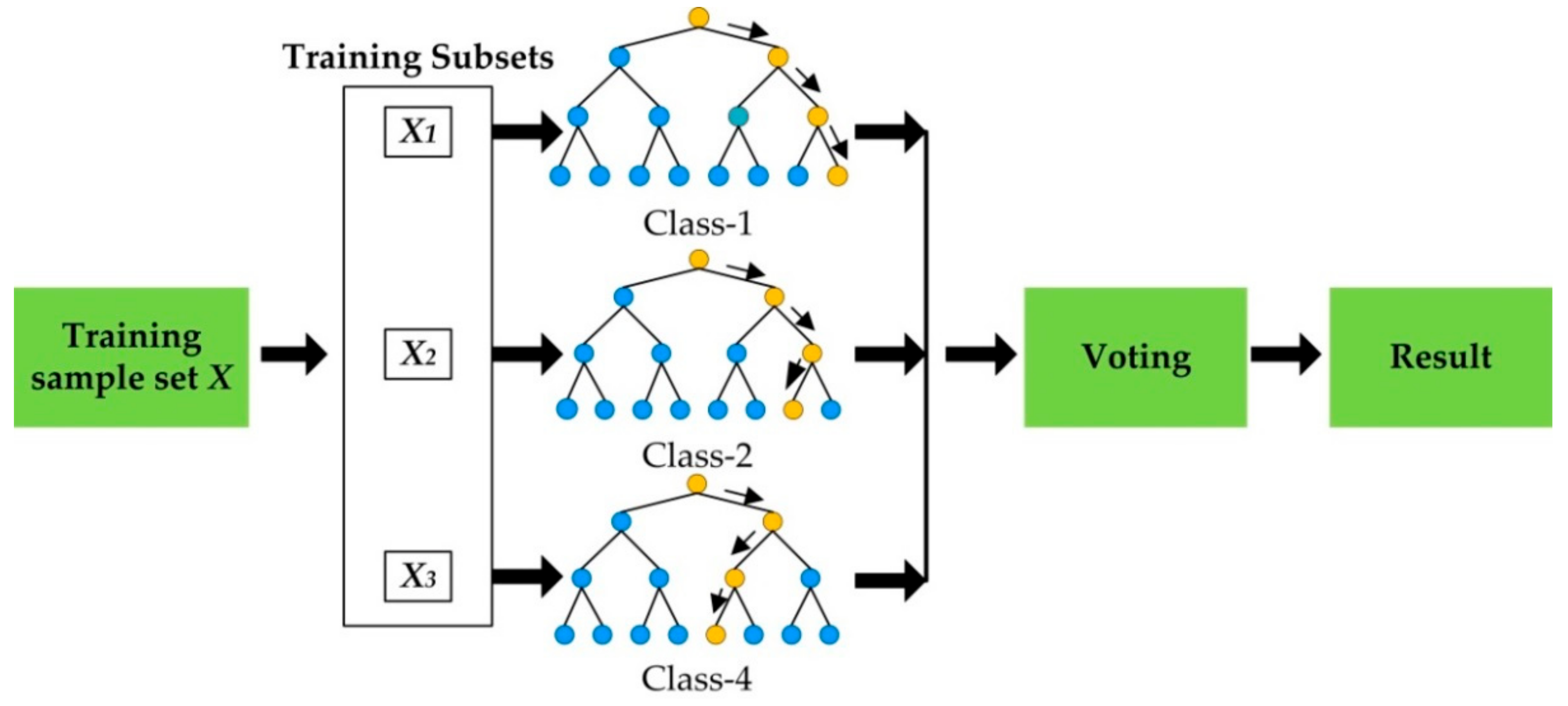
Accordingly, increasing the diversity of trees can improve the classification accuracy of the model. RF achieves this goal by training data set randomization and input variable set randomization. Figure 1 illustrates the model development procedure of RF. RF generates multiple new training data subsets by random extraction and substitution. The size of the training subsets is the same as that of the initial training data set, and repetitive training subsets are generated by extraction and substitution.
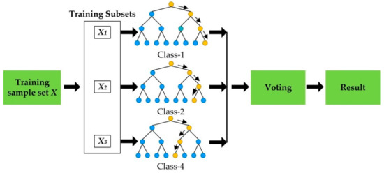
Figure 1.
The process of producing Random Forest (RF) results.
The new training subsets have, on average, 63.2% of the initial training data, with the rest as duplicates [30]. Since all the training subsets are randomly generated, the development of trees in RF is expected to be independent and different from each other. Once all the trees in the RF are established, the results of the classification will be voted on by all the trees. It can balance the impact of training data and make RF stable. The classification results from RF will also be more accurate than other methods.
3. Experiment Design
3.1. Experimental Condition
Two data sets were applied to verify the proposed method. Firstly, we applied the proposed method in a real environment to verify the practicability of the method. As for the actual operation, the number and state of load in the collected mixed data are unknown, so it is necessary to build the training data set by building load-signature database. The method of building load-signature database will be briefly introduced in Section 3.2. This specific work has been carried out by my colleagues in another article. Then, we applied the proposed method to public data set BLUED [31] to verify the generalization of the model. Furthermore, the method proposed in this paper was compared with the traditional methods [9,32] on the BLUED to show the progress of the method proposed in this paper.
The data set was built for NILM problem. The BLUED consists of voltage and current measurements for a single-family residence in the United States, sampled at 12 kHz on phase A and B for a whole week [31]. Every state transition of each appliance in the home during this time was labeled and time-stamped. There were a total of 2482 events (904 on phase A and 1578 on phase B). We chose the public data set BLUED because it better reflects the actual electricity consumption of ordinary households. Since it contains the state transition of most electrical appliances, we chose the fourth day data as training data. We took the collection data in the 18:48:26–18:50:25 period of the fifth day as test data. According to the above, the label of the training data set can be obtained directly.
3.2. Building of Load-Signature Database
In practical operation, it is impossible to directly obtain the operation states of independent load from mixed signals. Moreover, limitations are inevitable if prior data is used as training data. Different brands will cause a significant difference in the waveforms for the same type of load. Thus, this paper adopted a method that builds a load-signature database for the independent user.
This method established the corresponding signal template for each load in different users’ families. All the signal templates in a family make up a load-signature database for this family. Moreover, this method can update the database according to the newly added appliances in the family. The details of this method have been completed by my colleagues in another paper. This paper gives a brief introduction to this method.
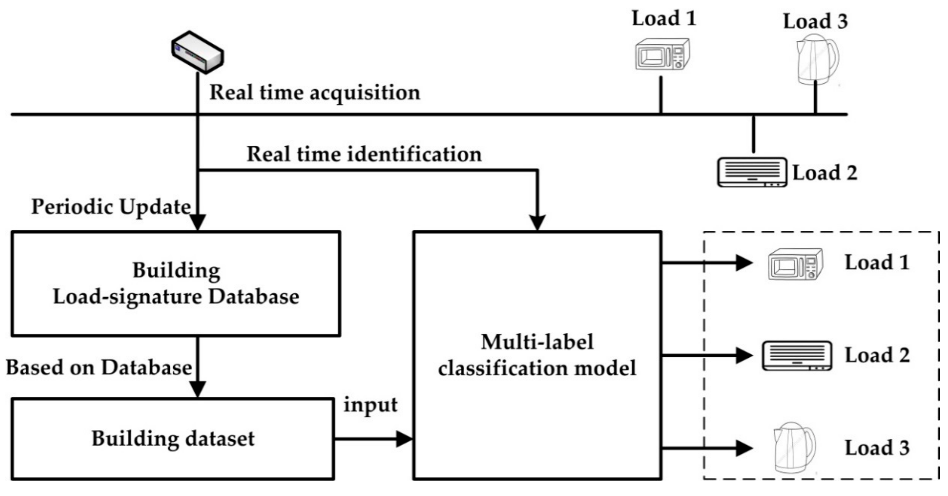
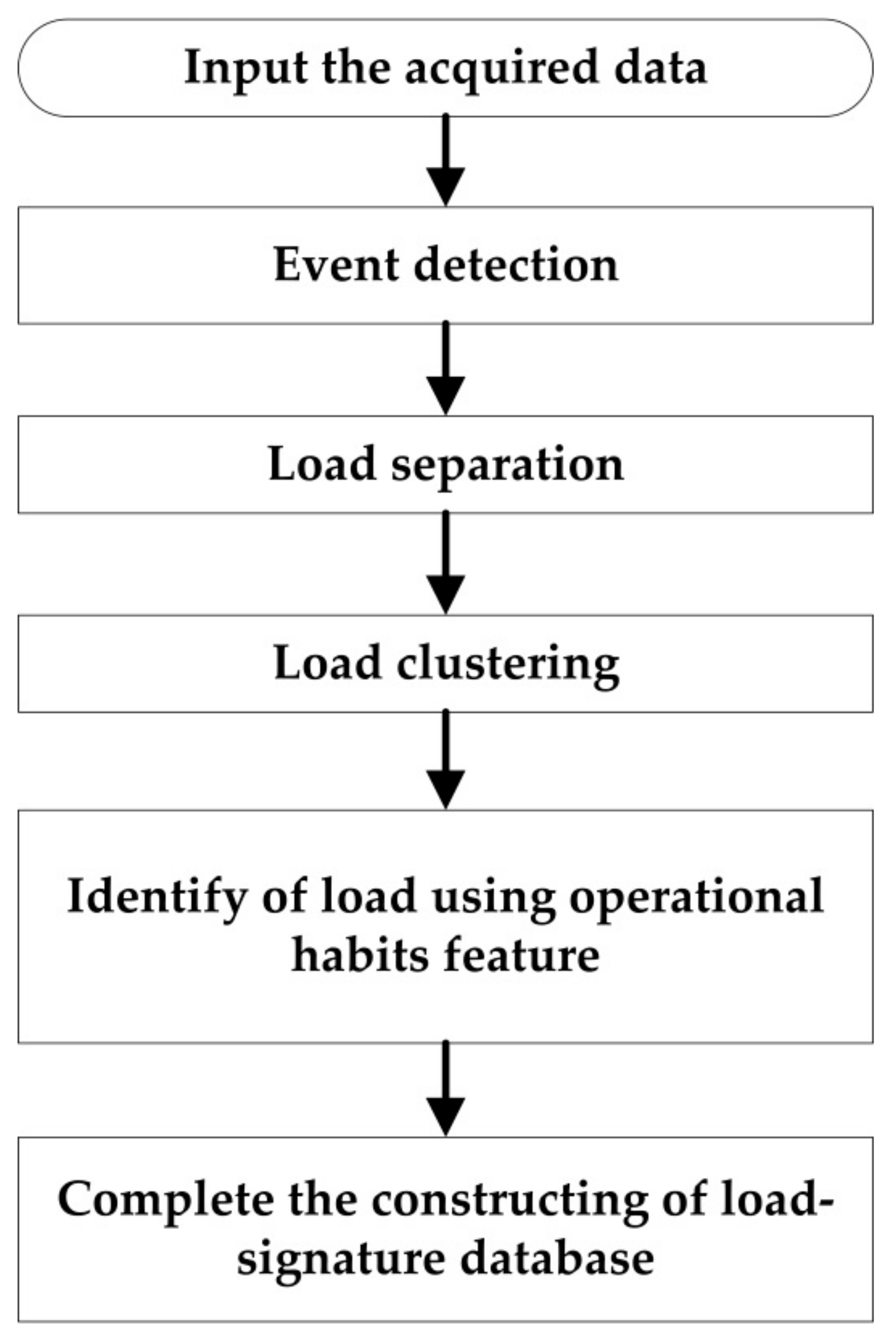
This method is based on high frequency data acquisition because high-frequency data can retain relatively complete load waveforms and signatures. After load decomposition is completed, load types are identified according to their inherent statistical signatures. At last, the load-signature database is built. The whole procedure of NILM by this method is shown in Figure 2. The process of building load-signature database is shown in Figure 3.

Figure 2.
Overall process of proposed method.
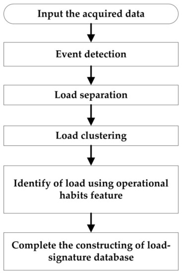
Figure 3.
The process of building load-signature database.
3.3. Building of Data Set
As a typical supervised learning method, multi-label classification requires data set to build the model. In this paper, data set was divided into two categories including training data set and test data set. The training data set was used to build model while the test set was used to evaluate the performance of the model for new data. The training data set consists of two parts: a set of sample data and a set of associated labels. For the test set, it contains only sample data. After the classification is built, it will be inputted. The output result will be analyzed to evaluate the performance of the model.
For NILM, the sample data is the basic electrical features extracted from mixed signal. In this paper, several basic electrical features were used to build models. They were represented by vector f.
where is the root mean square of current signal, is the crest factor of current signal, is the maximum value of current signal, is the real power, is reactive power, is power factor, is the fundamental wave and is the harmonics.
For f, can be obtained from current signal directly; can be obtained by calculation with current and voltage signal; can be obtained from FFT.
In mixed data, the running loads are labeled ‘1’, and the other loads are labeled ‘0’.
3.4. Feature Importance
The feature importance of RF uses data permutation to measure the influence of each feature on the final classification result of the model. The importance of features is obtained by calculating the reduction of classification accuracy caused by random permutation of features. The more the classification accuracy decreases, the more important the features are, and vice versa. The rationale is that the original association between a feature and the output could be broken by randomly permuting its values, and accordingly, the classification accuracy would decrease if the original feature is replaced by the permuted one [28].
Feature importance can be used to select the most important feature in RF. This will help users acquire the most important features on the results and understand the relationship between input and output. It is important for high-dimensional data set. In this paper, the feature importance is used to obtain the most influential feature of RF models.
3.5. Model Development
3.5.1. Multi-Label Classification Model
Multi-label classification is considered as a method of mapping from one sample to multiple labels. These multiple labels belong to same label set, in which the labels are inconsistent. The goal of multi-label classification is to build a classification model for unseen samples. It is divided into two categories: algorithm adaptation and problem transformation [29]. The algorithm adaptation method is to adapt and extend the existing single-label classification methods to meet the requirements of multi-label classification. The problem transformation is a method of transforming a multi-label classification problem into many single-label classification problems and solving the single-label classification problem with existing single-label classification algorithms. The method proposed in this paper is to use RF algorithm as classification algorithm in problem transformation method.
3.5.2. Important Parameters of Model
The establishment of RF requires three parameters. They are: the minimum number of terminal nodes for each tree (nodesize), the number of trees in the forest (ntree), and the number of randomly selected variables to grow the tree (mtry), respectively [30].
Nodesize controls the size of each tree in the RF. In other words, this parameter determines the stop time of the splitting process. A large nodesize will reduce the layer numbers of the tree and save computing time, but it will reduce the classification accuracy. In contrast, small nodesize increases the accuracy of RF classification, but it takes more time. Based on previous studies, this paper set nodesize as 5 [33].
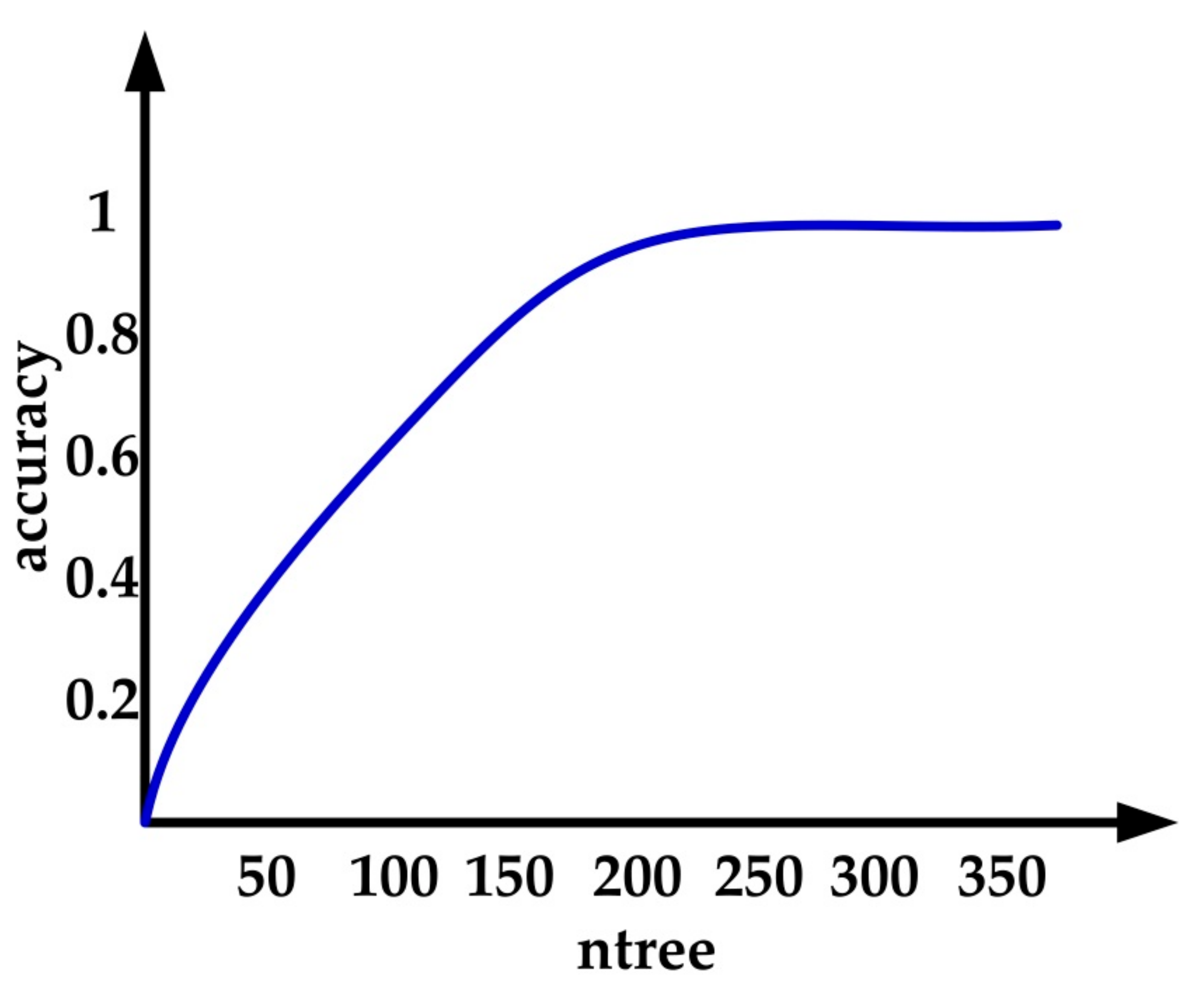
Ntree represents the number of decision trees in RF. A large ntree represents the large scale of trees in RF, which will improve the classification accuracy of RF, but results in an increase in computing time, and vice versa. In order to find a suitable ntree to balance accuracy and computation time, the authors have undertaken many experiments, and the results are shown in the Figure 4. As can be seen from Figure 4, when ntree is greater than 250, the accuracy is not significantly improved. Thus, the ntree was set as 250 in this paper.

Figure 4.
The classification accuracy of different number of trees in the forest (ntree) parameters.
Mtry parameter determines the size of randomly selected features; it impacts both the classification performance of the individual trees in the forest and the correlation between them, which jointly determine the classification accuracy of RF [34]. The trees in an effective RF have high classification accuracy with low correlation with each other. Generally, more features are selected, the classification performance of a single tree will be better, but it will cause the increase of correlation between each tree. Thus, in essence, the select of mtry is the balance between classification accuracy and correlation.
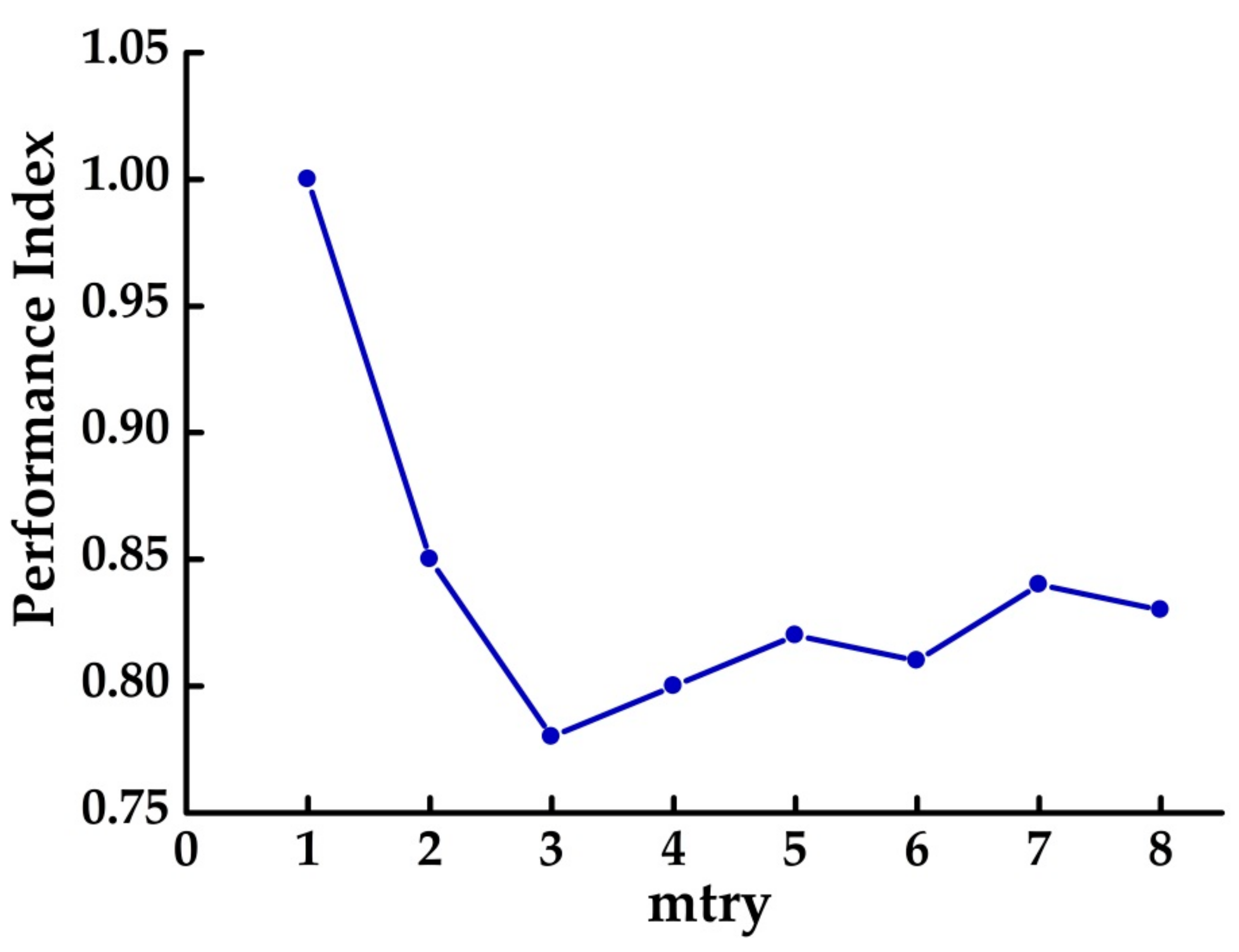
In this paper, a method is applied called k -fold cross-validation to obtain the appropriate mtry. Figure 5 shows the comparison results with different mtry. The curve shows the trend of the PI of RF trained with different mtry settings. As shown in the curve, when n is 3, the minimum PI is obtained, so the mtry of this paper was set as 3.
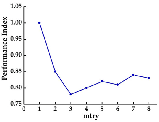
Figure 5.
Results for RF trained with different number of randomly selected variables to grow the tree (mtry) selections.
3.5.3. Evaluation of Model
There are many methods to evaluate multi-label classification algorithm, such as accuracy, Hamming distance loss, F-score and so on. This paper chose F-score and accuracy as the evaluation criteria of the algorithm, which will be introduced in the following.
This accuracy is used to evaluate the overall level of classification algorithm, representing the correct proportion of prediction results. It can be expressed by Equation (3):
where, TP and TN are the number of true positive and true negative while FP and FN are the number of false positive and false negative, respectively.
Before introducing F-score, several concepts need to be introduced. The first concept is Precision which represents the proportion of the true positive in all positive after identification calculated by Equation (4). And then, the Recall represents the proportion of positive samples that is correctly identified, which is calculated by Equation (5):
F-score is a measurement of P and R equilibrium. For multi-label classification, F-score has two forms. In this paper, label-based method was selected as it considers each output label. It is calculated by Equation (6):
where, L is the number of labels in data set, and are the Precision and Recall for label respectively.
4. Experimental Result
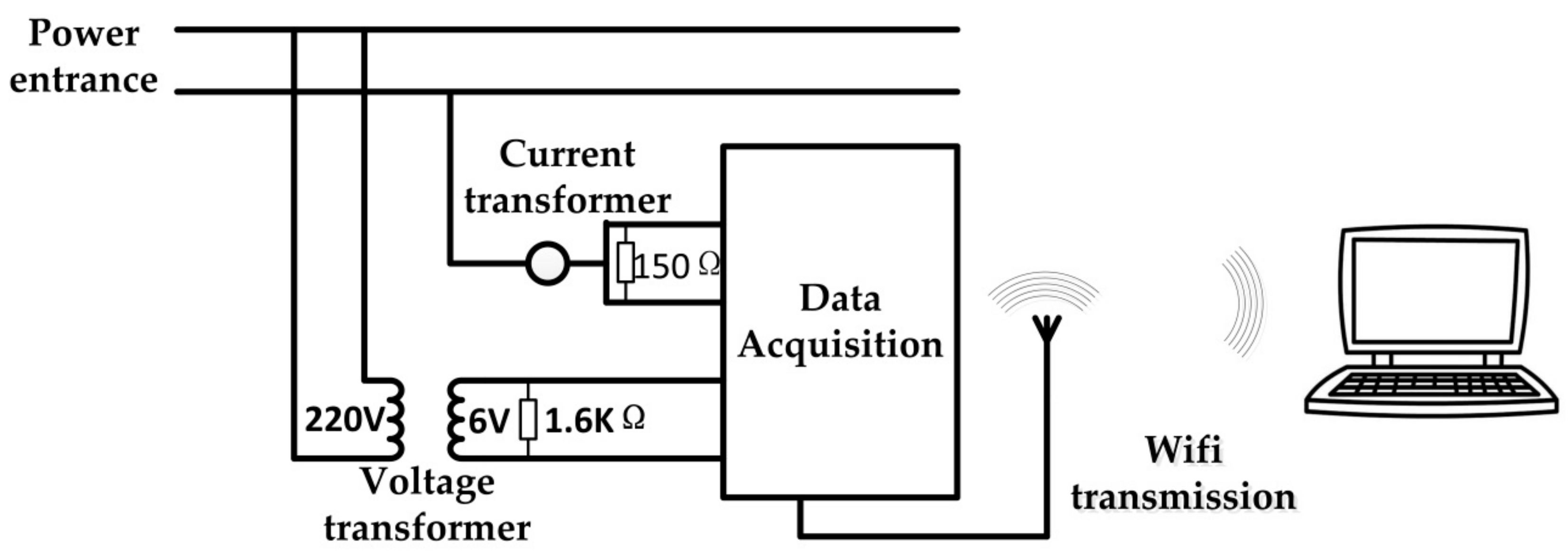
To verify the practicability of the proposed method, a data acquisition device is used to obtain actual data. Moreover, the construction of multi-label classification model will follow the processing flow proposed in this paper with obtained actual data. The data acquisition device is shown in Figure 6. The device consists of voltage, current transformers and data acquisition card. The voltage and current transformers reduce the intensity of signals acquisitioned. The EM-9636B was used as data acquisition card. Data acquisition card is responsible for collecting high-frequency data and transferring the collected data to the computer for subsequent processing.

Figure 6.
The data acquisition device.
4.1. Building Load-Signature Database for Laboratory
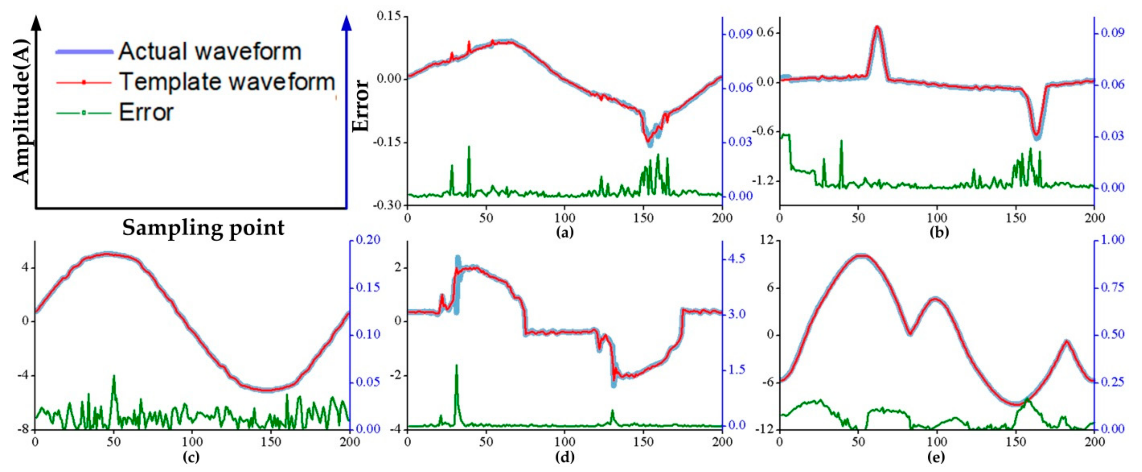
In this paper, data was obtained from laboratory and a load-signature database for laboratory was constructed according to the method in Section 3.2. In the database, there are five loads including: two computers of different brands, a printer, a kettle and a microwave oven. The Figure 7a–e shows the built load-signature database of the laboratory. The error between those loads’ signal templates and actual signal waveforms is also shown in Figure 7.

Figure 7.
The signal in load-signature database and actual waveform; (a) and (b) are the computers of different brand; (c) is the kettle; (d) is the printer; (e) is the microwave oven.
In the Figure 7 the blue waveform represents the signal obtained by data acquisition device when the load is working alone, while the signal templates obtained by proposed method in Section 3.2 denoted by red waveform. The waveform template and the corresponding actual waveform have very high similarity. Thus, the obtained template waveform can be used to replace the actual waveform.
4.2. Building of Data Set
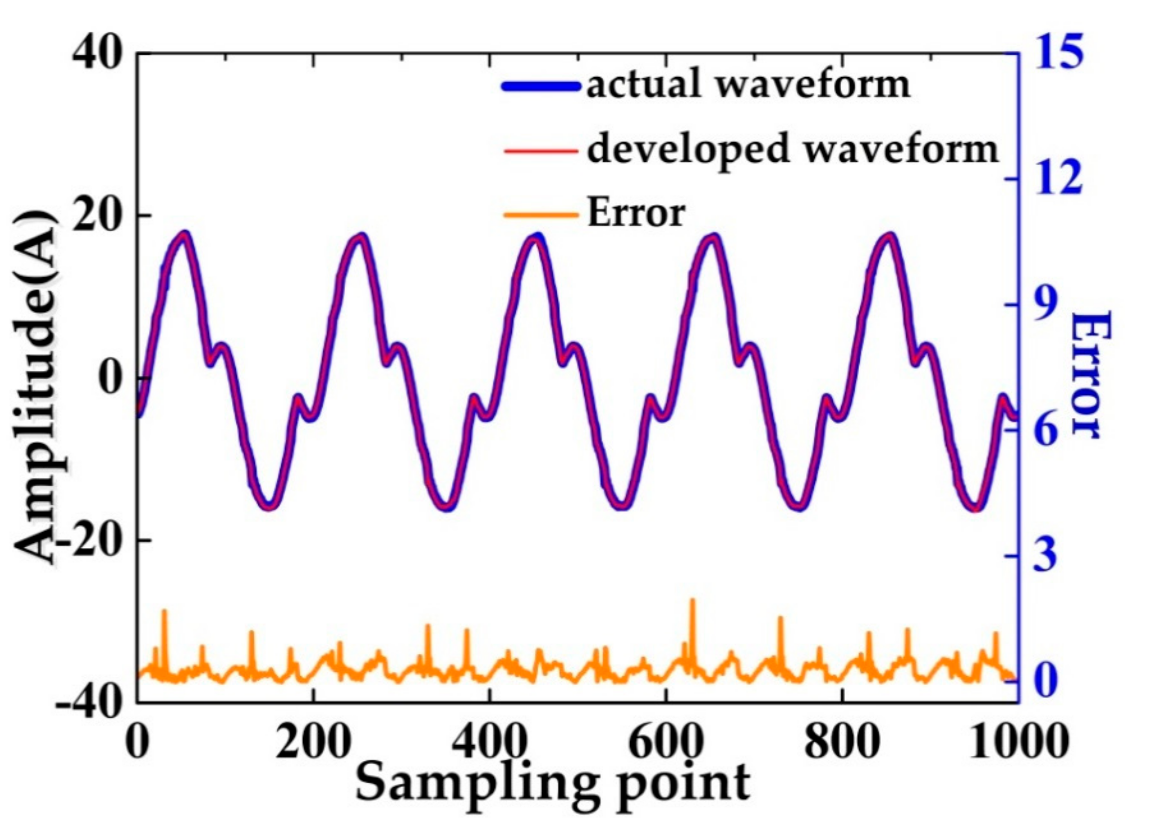
In Figure 8, the difference between developed waveform and actual waveform is shown. The blue waveform denotes the actual waveform when the same loads are working together; represented by red waveform, the developed waveform is obtained by superposition of signal templates of above loads to simulate reality. The low-power load and noise are the main reasons for the difference.

Figure 8.
The difference between developed waveform and actual waveform.
Table 1 shows the structure of training data set including two parts: features extracted from mixed signal and corresponding labels. The mixed signal obtained by superposition of the signal templates in the load-signature database. The labels of superimposed loads are “1”; the other loads’ labels are “0”. The features extracted from mixed signal will be used to identify the operating state of the load.

Table 1.
Part of built data set.
4.3. Feature Importance Comparison
Figure 9 shows each feature’s importance for building model. The IMAX and Har3rd have the biggest impact on results, reaching 20%, and the reactive power has little impact on results. The contributions of IRMS, and fundamental wave are both over 15%. The importance of crest factor, the real power, and the power factor is 6%, 10%, 9%, respectively. Q will not be considered in the next process of building the model.
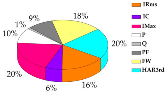
Figure 9.
The importance of different features.
4.4. Classification Algorithm Comparison
Two famous algorithms of algorithm adaptation method were chosen as contrast including: Multi-Label kNN (ML-kNN) and Back-Propagation Multi-Label Learning (BP-MLL). Three common problem transformation methods were applied in this paper (binary relevance method, classifier chain method and label power-set method).
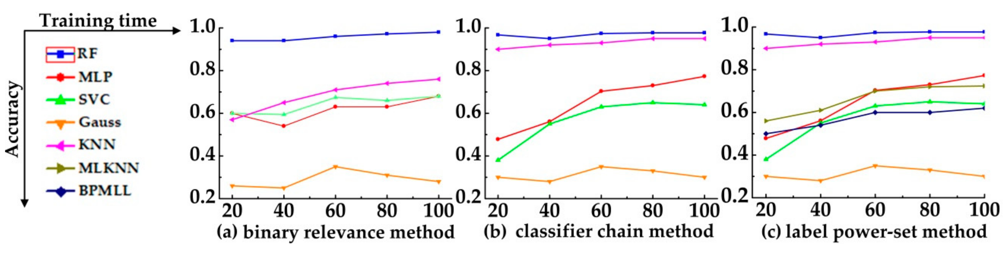
Figure 10 shows the identify accuracy of each multi-label classification algorithm. The (a) is the accuracy of binary relevance method with each classification algorithm, and the (b) and (c) are classifier chain method and label power-set method, respectively. In the (c), the ML-kNN and BPMLL of algorithm adaptation methods are compared too. As can be seen from the Figure 10, no matter which classification algorithm is used, the accuracy of RF algorithm is the highest.
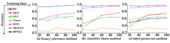
Figure 10.
The identify accuracy of each multi-label classification algorithm.
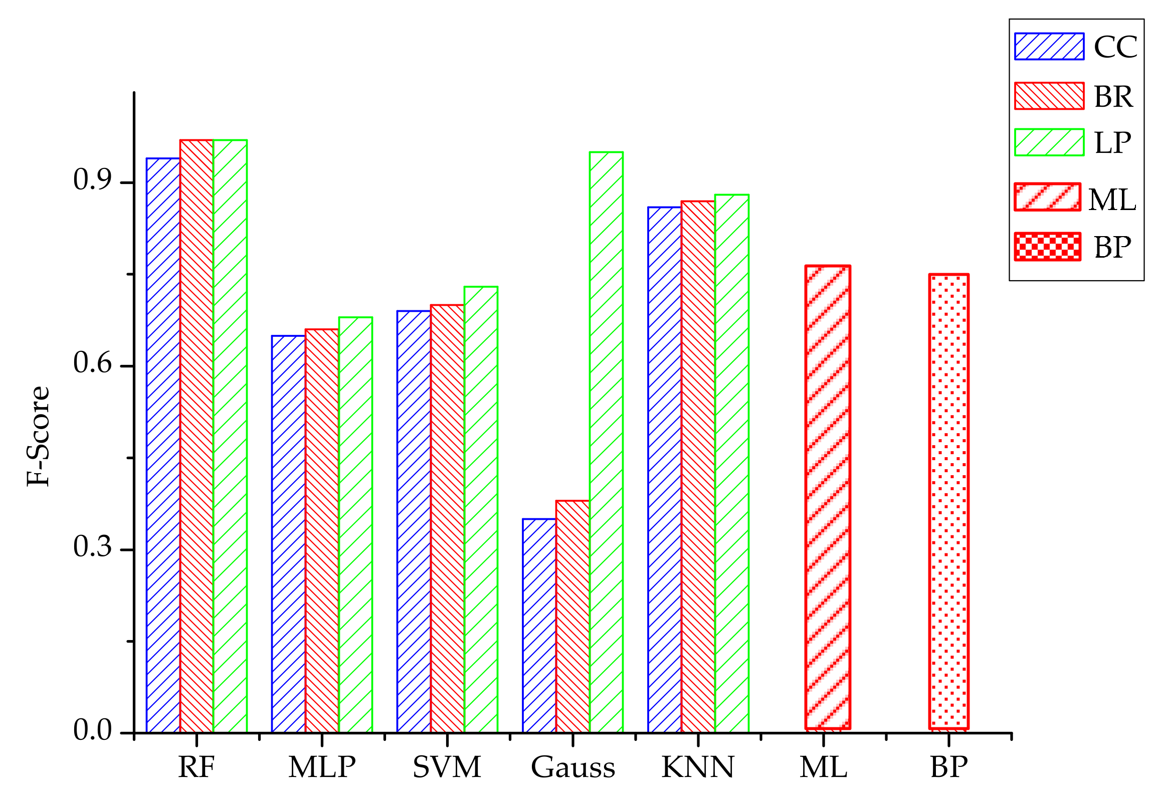
Figure 11 shows the F-Score of each multi-label classification algorithm. The RF algorithm still has the best performance, at almost 0.98.
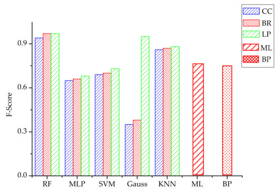
Figure 11.
The F-Score of each multi-label classification algorithm.
4.5. The Performance of RF for Test Data Set
Table 2 shows the building and identification time of multi-label classification model with RF algorithm in binary relevance method for actual data. The k-NN that performances better in other algorithms is tested as comparison. Table 2 indicates that RF also has advantages over k-NN in identification time, and the processing time has met the requirement of less than 2 s.
Table 2.
The comparison of data processing time.
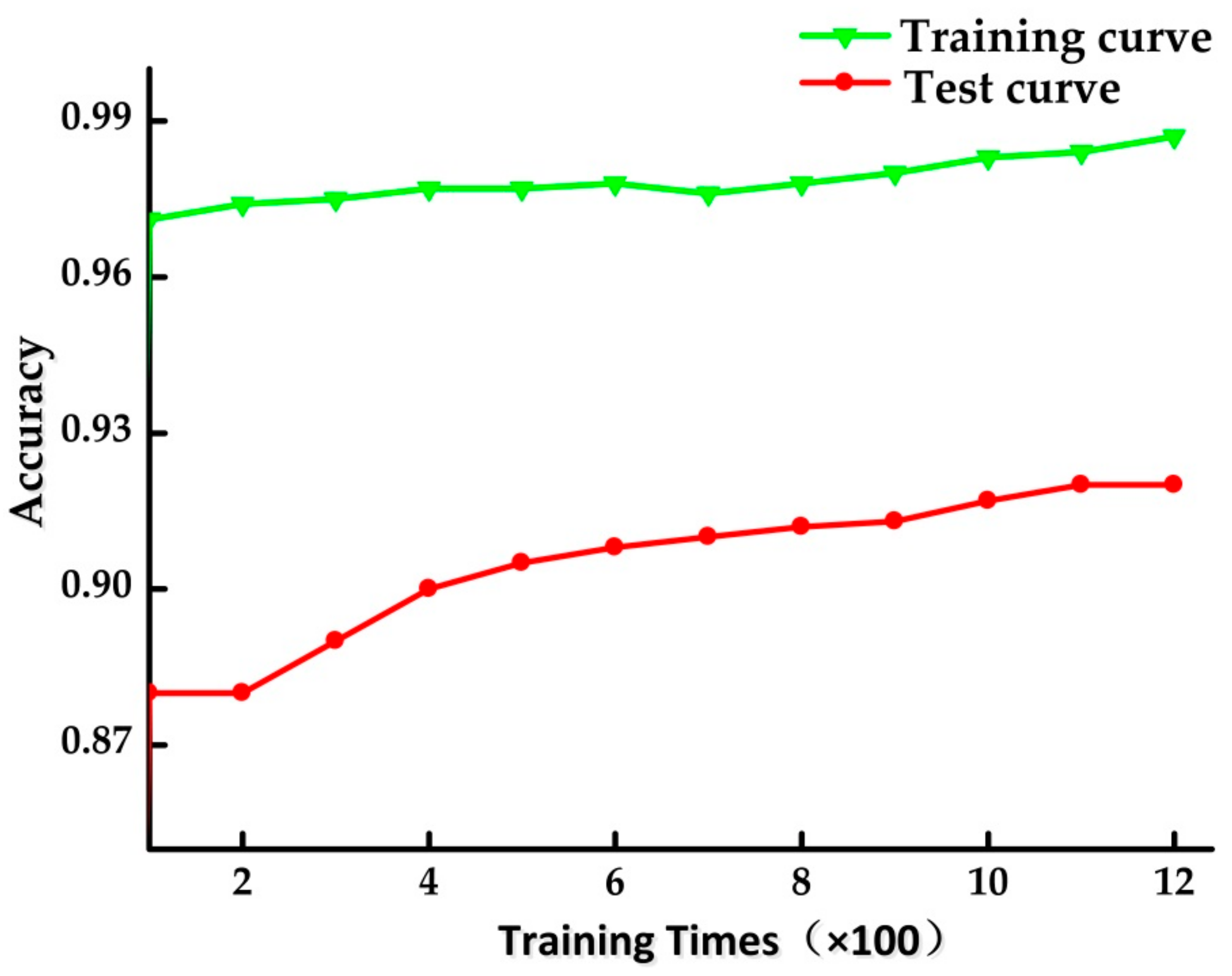
Figure 12 shows the performance of built multi-label classification model based on RF algorithm in binary relevance method for the test data set obtained from the laboratory. It indicates that the built model still has good performance in actual data. In Figure 12, the green curve represents the accuracy when the classification model is built by the training data set, while the accuracy of built model for test data set is denoted by red waveform. Although the accuracy of classification declined in the test of actual data, it still reached 92%. This proves that the identification method proposed in this paper is still effective in actual environment.
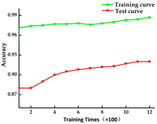
Figure 12.
The accuracy curve of built model.
4.6. Comparison with Other Methods
In this section, the traditional methods [9,32] were compared with our method on public data set BLUED. The method proposed by Tabatabaei [9] also uses the multi-label classification algorithm, the current and wavelet transform coefficients are used as training data. In the experiment of Tabatabaei’s work [9], ML-kNN algorithm achieves the best result. In the Bundit’s work [32], I, PF, Q, P are used as training data, and RAndom k-labELsets (RAKEL) achieves the best performance. Comparison is reflected in three aspects: accuracy, identification time and F-score for lamps. Table 3 shows the comparison result.
Table 3.
The comparison of data processing time.
From the comparison, it can be found that the proposed multi-label classification model based on RF has better performance than the traditional methods. Specially, although the overall accuracy of the method proposed by Bundit [32] is high, it does not have good performance in accuracy and F-score of low power electrical appliances (such as lamps). That is, the method proposed by Bundit [32] cannot accurately identify low-power electrical appliances, but the method proposed in this paper still performs well on low-power electrical appliances. Moreover, the proposed method takes less time, and therefore, it has higher efficiency.
5. Conclusions
Multi-label classification and non-intrusive load identification are naturally appropriate. There are two contributions in this paper, listed as followed: (1) the characteristics of NILM and multi-label classification are studied, and a multi-label classification model suitable for non-intrusive load identification is established. The model uses RF as classification algorithm; (2) feature importance is used as a criterion to select the most suitable features.
In this paper, RF algorithm is selected as the basic classification algorithm. In algorithm comparison, the RF algorithm outperforms other classification algorithms both in accuracy and F-score. The identification accuracy of RF is close to 0.97 and F-score is almost 0.98. For the actual data, the accuracy of binary relevance method with RF algorithm is close to 0.92. Moreover, in the process of model building and testing, the RF algorithm takes less time, which improves the identification efficiency. In comparison with existing methods, the experiment was conducted on public data set BLUED. The proposed method has better performance in accuracy, identification time and F-score for lamps than the other traditional methods [9,32]. The method proposed in this paper is superior to other methods especially in identifying low-power electrical appliances. Thus, multi-label classification method based on RF algorithm is efficient for NILM.
In order to further improve the accuracy of load identification, users’ habits and other features will be introduced into the classification model.
Author Contributions
X.W. and Y.G. conceived and designed the experiments; Y.G. performed the simulation; Y.G. and D.J. analyzed the results; and Y.G. and D.J. wrote and revised the paper.
Funding
This research was funded by [Natural Science Foundation of Beijing Municipality under grant] grant number [3172034] and [the Fundamental Research Funds for the Central Universities of China] grant number [2018MS001].
Conflicts of Interest
The authors declare no conflict of interest.
References
- Zhao, B.; Stankovic, L.; Stankovic, V. On a training-less solution for non-intrusive appliance load monitoring using graph signal processing. IEEE Access 2016, 4, 1784–1799. [Google Scholar] [CrossRef]
- Iglesias, F.; Palensky, P.; Cantos, S.; Kupzog, F. Demand side management for stand-alone hybrid power systems based on load identification. Energies 2012, 5, 4517–4532. [Google Scholar] [CrossRef]
- Chakraborty, D.; Elzarka, H. Advanced machine learning techniques for building performance simulation: A comparative analysis. J. Build. Perf. Simul. 2019, 12, 193–207. [Google Scholar] [CrossRef]
- Smarra, F.; Jain, A.; de Rubeis, T.; Ambrosini, D.; D’Innocenzo, A.; Mangharam, R. Data-Driven Model Predictive Control using random forest for building energy optimization and climate control. Appl. Energy 2018, 226, 1252–1272. [Google Scholar] [CrossRef]
- Madhur, B.; Francesco, S.; Rahul, M. DR-advisor: A data-driven demand response recommender system. Appl. Energy 2016, 170, 30–46. [Google Scholar]
- Hart, G.W. Nonintrusive appliance load monitoring. Proc. IEEE 1992, 80, 1870–1891. [Google Scholar] [CrossRef]
- Rahimpour, A.; Qi, H.; Fugate, D.; Kuruganti, T. Non-intrusive energy disaggregation using non-negative matrix factorization with Sum-to-k constraint. IEEE Trans. Power Syst. 2017, 32, 4430–4441. [Google Scholar] [CrossRef]
- Parson, O.; Ghosh, S.; Weal, M.; Rogers, A. An unsupervised training method for non-intrusive appliance load monitoring. Artif. Intell. 2014, 217, 1–19. [Google Scholar] [CrossRef]
- Tabatabaei, S.M.; Dick, S.; Xu, W. Toward non-intrusive load monitoring via multi-label classification. IEEE Trans. Smart Grid. 2017, 8, 26–40. [Google Scholar] [CrossRef]
- Rahimi, S.; Chan, A.D.C.; Goubran, R.A. Nonintrusive load monitoring of electrical devices in health smart homes. In Proceedings of the IEEE International Instrumentation and Measurement Technology Conference, Graz, Austria, 13–16 May 2012; pp. 2313–2316. [Google Scholar]
- Chahine, K.; Drissi, K.E.K.; Pasquier, C.; Kerroum, K.; Faure, C.; Jouannet, T.; Michou, M. Electric load disaggregation in smart metering using a novel feature extraction method and supervised classification. Energy Procedia 2011, 6, 627–632. [Google Scholar] [CrossRef]
- Rahayu, D.; Narayanaswamy, B.; Krishnaswamy, S.; Labbé, C.; Seetharam, D.P. Learning to be energy-wise: Discriminative methods for load disaggregation. In Proceedings of the 3rd International Conference on Future Energy Systems: Where Energy, Computing and Communication Meet, Madrid, Spain, 9–11 May 2012; pp. 1–4. [Google Scholar]
- Rahimi, S. Usage Monitoring of Electrical Devices in a Smart Home. Ph.D. Thesis, Carleton University, Ottawa, ON, Canada, 2012. [Google Scholar]
- Figueiredo, M.; de Almeida, A.; Ribeiro, B. Home electrical signal disaggregation for non-intrusive load monitoring (NILM) systems. Neurocomputing 2012, 96, 66–73. [Google Scholar] [CrossRef]
- Berges, M.; Goldman, M.; Matthews, H.; Soibelman, L.; Anderson, K. User-centered nonintrusive electricity load monitoring for residential buildings. J. Comput. Civil Eng. 2011, 25, 471–480. [Google Scholar] [CrossRef]
- Chang, H.; Lin, L.; Chen, N.; Lee, W. Particle-swarm-optimization-based nonintrusive demand monitoring and load identification in smart meters. IEEE Trans. Ind. Appl. 2013, 49, 2229–2236. [Google Scholar] [CrossRef]
- Chang, H. Non-intrusive demand monitoring and load identification for energy management systems based on transient feature analyses. Energies 2012, 5, 4569–4589. [Google Scholar] [CrossRef]
- Semwal, S.; Singh, M.; Prasad, R.S. Group control and identification of residential appliances using a nonintrusive method. Turk. J. Elect. Eng. Comput. Sci. 2015, 23, 1805–1816. [Google Scholar] [CrossRef]
- Srinivasan, D.; Ng, W.S.; Liew, A.C. Neural-network-based signature recognition for harmonic source identification. IEEE Trans. Power Deliv. 2006, 21, 398–405. [Google Scholar] [CrossRef]
- Ruzzelli, A.G.; Nicolas, C.; Schoofs, A.; O’Hare, G.M.P. Real-time recognition and profiling of appliances through a single electricity sensor. In Proceedings of the 7th Annual IEEE Communications Society Conference on Sensor, Mesh and Ad Hoc Communications and Networks (SECON), Boston, MA, USA, 21–25 June 2010; pp. 1–9. [Google Scholar]
- Du, L. Support vector machine-based methods for non-intrusive identification of miscellaneous electric loads. In Proceedings of the 38th Annual Conference on IEEE Industrial Electronics Society, Montreal, QC, Canada, 25–28 October 2012; pp. 4866–4871. [Google Scholar]
- Jiang, L.; Li, J.; Luo, S.; West, S.; Platt, G. Power load event detection and classification based on edge symbol analysis and support vector machine. Appl. Comput. Intell. Soft Comput. 2012, 2012, 27. [Google Scholar] [CrossRef]
- Hoogsteen, G.; Krist, J.O.; Bakker, V.; Smit, G.J.M. Nonintrusive appliance recognition. In Proceedings of the 3rd IEEE PES Innovative Smart Grid Technologies Europe (ISGT Europe), Berlin, Germany, 14–17 October 2012; pp. 1–7. [Google Scholar]
- Hosseini, S.M.; Carli, R.; Dotoli, M. Model predictive control for real-time residential energy scheduling under uncertainties. In Proceedings of the IEEE International Conference on Systems, Man, and Cybernetics (SMC), Miyazaki, Japan, 7–10 October 2018; pp. 1386–1391. [Google Scholar]
- Sperstad, I.B.; Korpås, M. Energy Storage Scheduling in Distribution Systems Considering Wind and Photovoltaic Generation Uncertainties. Energies 2019, 12, 1231. [Google Scholar] [CrossRef]
- Carli, R.; Dotoli, M. Energy scheduling of a smart home under nonlinear pricing. In Proceedings of the 53rd IEEE Conference on Decision and Control, Los Angeles, CA, USA, 15–17 December 2014; pp. 5648–5653. [Google Scholar]
- Wu, X.; Han, X.; Liu, L.Y.; Qi, B. A load identification algorithm of frequency domain filtering under current underdetermined separation. IEEE Access 2018, 6, 37094–37107. [Google Scholar] [CrossRef]
- Strobl, C.; Malley, J.; Tutz, G. An introduction to recursive partitioning: Rationale, application and characteristics of classification and regression trees, bagging and random forests. Psychol. Methods 2009, 14, 323–348. [Google Scholar] [CrossRef]
- Dietterich, T.G. An experimental comparison of three methods for constructing ensembles of decision trees: Bagging, boosting, and randomization. Mach. Learn. 2000, 40, 139–157. [Google Scholar] [CrossRef]
- Breiman, L. Bagging Predictors. Mach. Learn. 1996, 24, 123–140. [Google Scholar] [CrossRef]
- Anderson, K.; Ocneanu, A.; Benitez, D.; Carlson, D.; Rowe, A.; Berges, M. BLUED: A fully labeled public dataset for event-based non-intrusive load monitoring research. In Proceedings of the 2012 Workshop on Data Mining Applications in Sustainability (SustKDD 2012), Beijing, China, 12–16 August 2012. [Google Scholar]
- Bundit, B.; Waranyu, W.; Pattana, R. A non-intrusive load monitoring system using multi-label classification approach. Sustain. Cities Soc. 2018, 39, 621–630. [Google Scholar]
- Wang, Z.Y.; Wang, Y.R.; Zeng, R.C.; Srinivasan, R.S.; Ahrentzen, S. Random Forest based hourly building energy prediction. Energy Build. 2018, 171, 11–25. [Google Scholar] [CrossRef]
- Amit, Y.; Geman, D. Shape quantization and recognition with randomized trees. Neural Comput. 1997, 9, 1545–1588. [Google Scholar] [CrossRef]

© 2019 by the authors. Licensee MDPI, Basel, Switzerland. This article is an open access article distributed under the terms and conditions of the Creative Commons Attribution (CC BY) license (http://creativecommons.org/licenses/by/4.0/).