Filter Variable Selection Algorithm Using Risk Ratios for Dimensionality Reduction of Healthcare Data for Classification

Abstract

This research developed and tested a filter algorithm that serves to reduce the feature space in healthcare datasets. The algorithm binarizes the dataset, and then separately evaluates the risk ratio of each predictor with the response, and outputs ratios that represent the association between a predictor and the class attribute. The value of the association translates to the importance rank of the corresponding predictor in determining the outcome. Using Random Forest and Logistic regression classification, the performance of the developed algorithm was compared against the regsubsets and varImp functions, which are unsupervised methods of variable selection. Equally, the proposed algorithm was compared with the supervised Fisher score and Pearson’s correlation feature selection methods. Different datasets were used for the experiment, and, in the majority of the cases, the predictors selected by the new algorithm outperformed those selected by the existing algorithms. The proposed filter algorithm is therefore a reliable alternative for variable ranking in data mining classification tasks with a dichotomous response.

1. Introduction

The focus of this article is to design and test a filter algorithm that uses risk ratios (RR), otherwise known as relative risk, to rank the importance of predictor variables in data mining classification problems, with special attention to healthcare data. Variable importance ranking is the process that assigns numeric values, or some other form of quantifiers, to individual predictors in a dataset, indicating the level of their importance in predicting the outcome. After such a ranking has been established, variables that rank low can be expunged from a predictive model without compromising goodness of fit or predictive accuracy. Variable selection is necessary in the era of big data where voluminous data is generated from healthcare activities, including diagnosis, epidemiology analysis, and patient medical history. These data often consist of many attributes, some of which are not needed in data mining classification, and thus the need to select only the relevant ones is imperative.

Consider a dataset $D=\{(X_1,Y_1),\dots ,(X_m,Y_m)\}$ consisting of $m$ observations, where $X=(X_1,\dots ,X_n)$ are predictor variables having dimension $X\in R^n$ and $Y\in C$ where $C$ is a class label. In data mining, classification is defined as a mapping of the form $t:R^n\to C$ where $t$ is a classifier [1]. One of the ways of measuring the performance of a classifier is by evaluating its classification accuracy. That is, how accurately it can predict the classes of a set of vectors whose classes are unknown. The predictive accuracy of classification models is enhanced by the choice of variables used for model construction.

In [2], classification accuracy evaluation methods have been divided into two categories: scalar metrics and graphical methods. Scalar metrics compute accuracy by taking the ratio of correctly classified observations versus total number of observations in the validation set. For binary classification problems, scalar values representing accuracy are obtained from a confusion matrix, which is a tabulation of wrong and correct classification for each class [2,3]. In graphical methods, such as a receiver operating characteristics curve, accuracy is plotted on a $x,y$-axis to represent the tradeoffs between the cost of correct or wrong classification into class 0 or 1 [3].

The RR, just like odds ratios (OR), is a statistical measure of the association between binary variables across two different groups, where one group is referred to as the independent group while the other as the dependent group [4,5]. While odds ratios are known to overestimate the strength of association, the RR technique does not exhibit this demerit [6]. Additionally, odds ratios have the property of reciprocity, which allows for the direction of an association to be changed by taking the inverse of the OR estimate [6]. It turns out that RR does not exhibit this property. For the purposes of variable importance ranking, the direction of association is usually from independent variable to dependent variable and not vice versa; therefore, the lack of reciprocity in RR is a good property. Cashing in on the usefulness of the RR measure, this study will construct an algorithm that first binarizes data values of predictors in a dataset with a dichotomous response. Next, the algorithm evaluates the RR of each predictor with the response, and then outputs a value that signifies the relative importance of that predictor in determining the response. Computed values of RR will indicate the strength of the association, with larger values meaning strong association and, thus, high importance.

Literature evidence indicates that risk ratios have been deployed previously for different purposes within the healthcare domain. For example, [7] used RR to evaluate the extent to which red blood cells transfusion strategies are associated with the risk of infection among patients. The study, conducted on 7456 patient records, concluded that irrespective of the strategy used, blood transfusion was not associated with reduced risk of infection, generally. However, transfusion strategies were found to be associated with a minimized risk of specifically dangerous infections. In a related study, [8] used RR to investigate the relationship between caregiving and risk of hypertension incidence among American older adults. The research, conducted on 5708 Americans aged 50 years and above, held that caregiving for a spouse is associated with the possibility of becoming hypertensive by the caregiver in the long run. The association between diabetes and the possibility of prostate cancer incidence was investigated by [9] using RR. The research reported risk ratios representing the extent of this association as 5.83, 2.09, and 1.35 for ages 40–64, 65–70, and 75 years and above, respectively, on a sample of 1 million Taiwanese patients.

The aforementioned applications of RR in the healthcare domain give evidence that this technique holds good prospects for further deployment in this area. To our knowledge, risk ratios have so far been applied only in cohort and specific studies, with results limited in scope and generalization potentials. Against this backdrop, this research will explore the possibility of using the RR as the basis for developing a generic variable importance ranking algorithm. The algorithm will facilitate reduction of the dimension space of any healthcare dataset in order to enhance predictive accuracy and efficiency.

There are basically three categories of variable selection methods: filter, embedded, and wrapper [10]. The filter methods do not depend on any machine learning algorithm [11]. Filters are executed on raw datasets as a form of preprocessing in order to determine the appropriate predictor subset that will produce the most accurate classification results. On their own, filter algorithms cannot tell how effective a selected subset can be for model construction, unless a particular learning algorithm is deployed. Embedded methods are dependent on particular machine learning models. They incorporate variable selection mechanisms into the model construction algorithms such that learning and variable selection work hand-in-hand [10]. Wrapper methods scan through the variable space, evaluating different subsets using the machine learning algorithm itself to determine the subset that produced the best-performing model [12]. Three commonly used techniques of wrapper methods are forward selection, backward elimination, and recursive elimination.

2. Literature Review

This section covers the review of existing variable selection techniques relevant to this research. The materials to be used in the design of the proposed algorithm and for testing its effectiveness are also presented in this section.

2.1. Filter Methods of Variable Selection

According to [12], filter methods of variable selection use statistical techniques to evaluate the correlation of each predictor with the outcome variable. Filtering attempts to find a subset of attributes that are highly correlated with the class variable but at the same time exhibits low inter-correlation among each other [13]. This process of variable selection does not work in conjunction with any classification algorithm. It is after the best attributes have been filtered out that a machine learning algorithm can be deployed to perform classification on the best variables. Some commonly used filter methods are the Fisher score and Pearson’s correlation. These algorithms achieve variable selection in a supervised manner.

Fisher Score. For a dataset with binary class (0/1), the Fisher score $(F_i)$ evaluates the importance of the $i$-th predictor by using Equation (1):

$$F_i=|\frac{{\overline{X}}_1(i)-{\overline{X}}_0(i)}{d_1^2(i)-d_0^2(i)}|$$

(1)

where ${\overline{X}}_1(i)$ and $d_1(i)$ are the mean and standard deviation of the $i$-th predictor in class 1, respectively; while ${\overline{X}}_0(i)$ and $d_0(i)$ are the same parameters in class 0 [14]. Higher Fisher scores indicate that a variable is strongly associated with the outcome variable.

Pearson’s Correlation. One of the correlation-based filter techniques is the Pearson correlation, given in Equation (2) [15].

$$P_i=\frac{Cov(X_i,Y)}{\sqrt{Var(X_i)\times Var(Y)}}$$

(2)

where $X_i$ is the $i$-th feature, $Y$ is the class label, and $Cov()$ and $Var()$ are the covariance and variance, respectively. This measure ranks predictor variables according to their individual linear dependence with the output variable.

2.2. Unsupervised Variable Selection

Automatic Variable Selection. The R programming language, developed by R Core Team, [16], has a package called leaps that consists of a function, regsubsets, used for automatic selection of best variables [17]. The function can be used to achieve variable selection in either of three ways: by specifying the maximum number of best variables to return, by forward selection, and by backward elimination. In order to select the best subset of a particular size, the number of desired variables is specified in the nvmax argument.

Another alternative is to utilize the regsubsets function to perform forward selection or backward elimination in selecting subsets according to their importance. When this is executed, the function selects and returns the most important variables for modeling. Apart from selecting the best subsets, regsubsets ranks select variables according to importance. This is done by indicating against each variable one or more asterisks. The number of asterisks assigned to a variable is proportional to its importance.

Variable Importance Measure. The R language consists of another package, known as caret for Classification And REgression Training [18]. One of the functions within the caret package is the varImp (variable importance), which implements variable importance ranking for different machine learning algorithms, such as Logistic regression and Random Forest. To evaluate the importance of variables in a Random Forest model using varImp, the importance of a predictor variable $X_j,j=1,\dots ,n$ is calculated on the out-of-bag (OOB) data sample for each tree that was not used for tree construction. Initially, the predictive accuracy of the OOB sample is evaluated. Then, the values of $X_j$ in the OOB are permuted; keeping all other predictor variables unchanged. The predictive accuracy of the shuffled data values is also measured and the mean predictive accuracy across all trees is reported. By doing so, the importance of a variable in predicting the response is quantified by evaluating the difference of how much including or excluding that variable decreases or increases accuracy [18,19,20]. This difference is referred to as the Mean Decrease Accuracy (MDA), and is computed by the formula shown in Equation (3) [21,22].

$$I(X_j)=MDA(X_j)=\frac{1}{n}{\displaystyle \sum _{t=1}^n\frac{{\displaystyle \sum _{i\in OOB}I(y_i=b(X_i))-{\displaystyle \sum _{i\in OOB}I(yi=a(X_i^j))}}}{\left|OOB\right|}}$$

(3)

where $n$ is the total number of trees and $t$ is a particular tree, $t=1,\dots ,n$. In Equation (3), $y_i=b(X_i)$ is the predictive accuracy for OOB instance $X_i$ before permuting $X_j$ and $y_i=a(X_i^j)$ is the predictive accuracy for OOB instance $X_i$ after permuting $X_j$, while $\left|OOB\right|$ is the number of data samples not used in tree construction.

In the case of Logistic regression models, the varImp function evaluates the importance of a predictor variable using the absolute value of the $t$-statistic for that predictor.

2.3. Relative Risk (RR)

The formal definition of Relative Risk to be used in the algorithm design is given as: Let $t_{11}$= total data points where $X=1$ and $Y=1$, $t_{10}$ = total data points where $X=1$ and $Y=0$, $t_{01}$= total data points where $X=0$ and $Y=1$, and $t_{00}$ = total data points where $X=0$ and $Y=0$ for a binary independent variable $X$ and a binary dependent variable $Y$. Then, the relative risk is given by

$$RR=\frac{t_{11}/(t_{11}+t_{10})}{t_{01}/(t_{01}+t_{00})}=\left(\frac{t_{11}}{t_{11}+t_{10}}\right)·\left(\frac{t_{01}+t_{00}}{t_{01}}\right).$$

(4)

The relative risk in Equation (4) is represented in tabular form as shown in

Table 1. Tabular definition of relative risk (RR).

	$\mathit{Y}=1$	$\mathit{Y}=0$	Total
$X=1$	$t_{11}$	$t_{10}$	$t_{11}+t_{10}$
$X=0$	$t_{01}$	$t_{00}$	$t_{01}+t_{00}$

[4,5,23].

The independent variable,$X$, is referred to as the exposure, with 0 and 1 as the unexposed and exposed, respectively. On the other hand, the dependent variable, $Y$, is referred to as the incidence or risk of an event among the various exposure groups, with 0 and 1 representing event failure and success, respectively [4]. Relative risk measures the ratio of the incidence of an event among data points within the exposed group compared with the incidence of that same event in the unexposed group [5,23]. Exposure in this context could be any criterion of measurement by which data is generated. The RR values range from 0 to infinity, where RR = 1 signifies that no association exists between $X$ and $Y$, RR < 1 indicates a negative association between $X$ and $Y$, and RR > 1 shows that $X$ and $Y$ are positively associated [23,24,25].

2.4. Classification Tools

Logistic regression is a modeling tool used in examining the association between a categorical dependent variable and one or more independent variables of a set of observations [26]. This regression type is anchored on the logistic function where values must lie between 0 and 1, corresponding to class labels. The probabilities indicating the possibility of an observation belonging to a certain class are modeled using the logistic equation, $\log \left(\frac{P}{1-P}\right)=b_0+b_1{X}_1+\dots +b_n{X}_n,$ where $P$ is the probability of success, $P/(1-P)$ is the odds, $b_0$ is the intercept, $b_1,\dots ,b_n$ are parameter estimates, and $X_1,\dots ,X_n$ are data values corresponding to each independent variable [27,28].

Meanwhile, Random forest is a machine learning tool that combines many tree predictors $\{h(X,v_k),k=1,\dots ,n\}$, where $X$ is an input vector and $\left\{v_k\right\}$ are independent random vectors within the same distribution across all trees in the forest [1,29]. In order to determine the class of an input vector $X$, each tree casts a single vote and the class with more votes is selected [1].

Predictive Accuracy. The predictive accuracy and the balanced classification accuracy (BCA) are defined by

$$Accuracy=\frac{T^{+}+T^{-}}{T^{+}+T^{-}+F^{+}+F^{-}}$$

(5)

and

$$BCA=0.5\times \left[\frac{T^{+}}{T^{+}+F^{-}}+\frac{T^{-}}{T^{-}+F^{+}}\right]$$

(6)

respectively, where, $T^{+}$ is the number of correctly classified observations in class 1, $T^{-}$ is the number of correctly classified observations in class 0, $F^{+}$ is the number of observations in class 0 but wrongly classified in class 1, and $F^{-}$ is the number of observations in class 1 but wrongly classified in class 0 [30].

3. Methodology

3.1. Experimental Datasets

A number of datasets, mostly from the healthcare domain, were deployed to demonstrate the effectiveness of the proposed algorithm in feature selection. Since the proposed algorithm places emphasis on a dichotomous response, each experimental dataset considered in this experiment has a binary outcome. The considered datasets are listed below:

• Psychological Capital (PsyCap). This dataset carries psychological capital (PsyCap) information of some workers in the hospitality industry. Psychological capital measures the capabilities of an individual that enable them to excel in the work environment [31]. Each worker’s PsyCap was assessed on the four components of psychological capital (hope, efficacy, resilience, and optimism), using the questionnaire presented in [32]. The workers willingly completed the questionnaires and returned the same, and there were no requirements for prior ethics approval. The dataset has a binary class variable, where 0 and 1 represent low and high PsyCap, respectively.
• Diabetes in Pima Indian Women (Diabetes). The dataset consists of 332 observations about diabetes test results of Indian women of Pima indigene. The population sample was those from 21 years and above, residing in Arizona. This dataset, accessible through the R language “MASS” package, reported in [33], is named Pimat.te within the package, and was originally sourced from [34]. The dataset has a binary response variable named “type”, where 0 and 1 signify non-diabetic and diabetic, respectively.
• Survival from Malignant Melanoma (Melanoma). This dataset, available in the R package “boot”, records information on the survival of patients from malignant melanoma [35]. The patients had surgery at the Department of Plastic Surgery of the University Hospital, Odense, Denmark, between 1962 and 1977. Several measurements were taken and reported as predictor variables, with a binary class “ulcer”, where 1 indicates an ulcerated tumor and 0, non-ulcerated.
• Spam E-mail Data (Spam). The dataset consists of e-mail items with measurements relating to total length of words written in capital letters, numbers of times the “$” and “!” symbols occur within the e-mail, etc.; and a binary class variable, “yes”, with 1 classifying an e-mail as spam and 0 otherwise. The dataset, titled spam7, can be accessed in the R package “DAAG” [36].
• Biopsy Data of Breast Cancer Patients (Cancer). Named biopsy in the R package, “MASS” in [33], the dataset measures the biopsies of breast tumors on a number of patients. The dataset was obtained from the University of Wisconsin Hospital, Madison, with known binary outcome named “class”, where 0 = benign and 1 = malignant.

Some characteristics of the experimental datasets are presented in

Table 2. Properties of the experimental datasets.

Dataset	Predictors	Records	Class 0	Class 1
PsyCap	20	329	68	261
Diabetes	7	332	223	109
Melanoma	6	205	115	90
Spam	6	4601	2788	1813
Cancer	9	683	444	239

.

3.2. Design of Proposed Algorithm

In this section, we will consider $X_j$, $j=1,\dots ,n$ as a set of predictors in a high dimensional space $R^n$. In most cases, especially with big data, some of these predictors are irrelevant, duplicative, and, thus, not needed in machine learning tasks [37]. Usually, the objective is to reduce the number of predictors to $k$ where $k<n$, such that $k$ consists of the most relevant explanatory variables needed in classification. This is the objective the proposed algorithm seeks to achieve.

Let RawData denote a dataset consisting $m$ observations, $n$ predictors, and the outcome variable $y_i$. Let RawDat$[i,j]$ denote a data point at row $i$, column $j$ where $i=1,\dots ,m$ and $j=1,\dots ,n$.

Preprocessing. This algorithm will require a normalized dataset on the interval [0,1], also referred to as min-max normalization [38,39]. The proposed algorithm, presented in Appendix A, will take the following steps:

• The first step of the proposed algorithm, as presented in Listing 1, is to binarize the dataset. It is a requirement that both independent and dependent variables carry only binary values for the risk ratio measure to be deployed. On purpose, we did not design the algorithm to print the output of the binary dataset. This is to guard against users inadvertently using the binary dataset for model construction. The binary data is only useful for RR computation, after which classification models are fit on the original dataset.
• In the second step, listed in Listing 2, the algorithm counts, for each predictor $X$ and the class $Y$, all occurrences where $(X,Y)=\left(1,1\right),\left(1,0\right),\left(0,1\right)\mathrm{and}\left(0,0\right).$ Just as in step 1, these computations are kept behind the scene, without printing any output visible to the user.
• The third step, listed in Listing 3, applies the risk ratio formula of Equation (4) on the values computed in Listing 2 to produce the variable importance rankings. This algorithm outputs the importance rankings of the variables in the order the predictors appear in the dataset. For a better view of the results, the user may decide to arrange the output in ascending or descending order. It is upon the judgment of the modeler to determine the cutoff point of those variables to include in a model.
• The statement on line 44 of the algorithm, in Appendix A, will output the names of predictor variables and their RR values, separated by a tab, each on a separate line. Each RR value constitutes the importance rank of the corresponding predictor, signifying the extent to which it is associated with the class.

The processes involved in feature ranking by the proposed algorithm are shown in the pseudo code below:

Algorithm 1. Pseudo code

START Convert dataset to binary, that is, round all values < 0.5 to 0 and > = 0.5 to 1 FOR each input/output, DO the following: IF INPUT is 1 AND OUTPUT is 1 THEN Count $t_{11}$ that is ${\delta }_j={\delta }_j+1$ ELSE Count $t_{10}$, that is ${\beta }_j={\beta }_j+1$ END IF IF INPUT is 0 AND OUTPUT is 1 THEN Count $t_{01}$ that is ${\varphi }_j={\varphi }_j+1$ ELSE Count $t_{00}$, that is ${\phi }_j={\phi }_j+1$ END IF NEXT input/output IF All input/output are exhausted, compute the following: FOR each variable $j=1$ to $n$ lowerSum ${}_j={\delta }_j+{\beta }_j$ upperSum ${}_j={\varphi }_j+{\phi }_j$   ${\mathrm{firstRatio}}_j=\frac{{\delta }_j}{{\mathrm{lowerSum}}_j}$ ${\mathrm{secondRatio}}_j=\frac{{\mathrm{upperSum}}_j}{{\varphi }_j}$   $VI{M}_j$ = $firstRati{o}_j\times secondRati{o}_j$ 21.   PRINT $columnNam{e}_j$ and space, and ${\mathrm{VIM}}_j$ 22. NEXT variable 23. STOP

A higher value of VIM for a predictor signifies strong association with the class, and consequently indicates its importance in classification. This algorithm is summarized in Equation (7).

$$VI{M}_j=\left(\frac{{\displaystyle \sum _{i=1,j=1}^{m,n}\delta ij}}{{\displaystyle \sum _{i=1,j=1}^{m,n}\delta ij}+{\displaystyle \sum _{i=1,j=1}^{m,n}\beta ij}}\right)·\left(\frac{{\displaystyle \sum _{i=1,j=1}^{m,n}\varphi ij}+{\displaystyle \sum _{i=1,j=1}^{m,n}\phi ij}}{{\displaystyle \sum _{i=1,j=1}^{m,n}\varphi ij}}\right)$$

(7)

where $VI{M}_j$ is the importance ranking of the jth predictor, $j=1,\dots ,n$, ${\mathsf{\delta }}_{ij}$ is the total number of observations with input = 1 and output = 1, ${\beta }_{ij}$ is the total number of observations with input = 1 and output = 0, ${\varphi }_{ij}$ is the total number of observations with input = 0 and output = 1, and ${\phi }_{ij}$ is the total number of observations with input = 0 and output = 0.

3.3. Experiment and Results

Execution of the Proposed Algorithm on the Datasets. The proposed algorithm was executed on all the datasets in order to rank the variables according to importance. The existing varImp function and the regsubsets methods (nvmax, forward, backward) were also deployed to rank the variables. Equally, the Fisher score and Pearson’s correlation were deployed. This was done in order to compare the effectiveness of the proposed algorithm against existing methods of variable selection.

Two machine learning algorithms, namely Logistic Regression and Random Forest, were used in the experiment for model construction, evaluation of goodness of fit, and predictive accuracy. Samples of variable ranking results on the Diabetes and Melanoma datasets are shown in

Table 3. Variable ranking results of Diabetes and Melanoma datasets.

Diabetes Dataset				Melanoma Dataset
Proposed Algorithm		varImp in Caret		Proposed Algorithm		Fisher Score
Variable	Ranking	Variable	Ranking	Variable	Ranking	Variable	Ranking
Glu	3.8438	Glu	43.4587	thickness	2.5556	thickness	0.4200
Npreg	3.7508	Age	21.0085	sex	1.5262	time	0.1500
Bmi	3.5803	Bmi	16.4553	age	1.2159	status	0.1500
Ped	3.4098	Skin	10.4756	year	1.1561	sex	0.0580
Age	2.4550	Npreg	7.9362	status	0.6324	age	0.0320
Skin	2.0050	Pped	7.1898	time	0.5242	year	0.0022
Bp	1.2672	Bp	−1.6153

.

Performance evaluation of the proposed algorithm in comparison with existing algorithms was done in two steps. First, the goodness of fit of models developed using variables selected by the new algorithm and existing ones was examined, and secondly, the predictive accuracy evaluation was carried out.

Goodness of Fit Evaluation. The goodness of fit test was assessed on two metrics: deviance and Mean Squared Error (MSE). In Logistic regression models, two deviance types are reported: null deviance and residual deviance [40]. The residual deviance is calculated cumulatively as predictors are added to the model. The difference between the final residual deviance and the null deviance explains the goodness of fit of a model. When comparing two models, the model with the smallest deviance is said to have better fit. The MSE is a parameter-free measure that gives information on the difference between actual and predicted values [41]. Lower values of MSE for a model indicate better fit. A sample result of the goodness of fit test of the various models is presented in

Table 4. Goodness of fit evaluation according to varlmp and the proposed algorithm.

varImp				Proposed Algorithm
Dataset	Subset Size	Deviance	MSE	Subset Size	Deviance	MSE
PsyCap	8	231.9	1.4	8	204.1	1.2
Diabetes	3	87.5	0.83	3	92.7	0.73
Melanoma	5	49	1.2	5	37.3	1.1
Spam	3	1017.7	1.3	3	929	1.4
Cancer	5	638.4	1.7	5	631.4	1.1

.

The goodness of fit results presented in Table 4 show that the subsets selected by the proposed algorithm competed favorably with those selected by the existing varImp algorithm.

Predictive Accuracy Evaluation. The results of the predictive accuracy test of models constructed with subsets selected by the proposed algorithm compared with those constructed with variables selected by existing algorithms were examined. Before fitting the models, each dataset was split into 80% and 20% train and test sets, respectively. The train sets were used for model construction, while the test sets were used to evaluate the predictive power of the models. Typically, the predictive accuracy is computed using Equation (5). However, Equation (5) assumes that classes of the dataset are balanced. This is usually not the case in real life as could be seen in Table 2, where the number of observations in class 0 is not same as that in class 1 across all experimental datasets. For imbalanced datasets, the balanced classification accuracy (BCA) defined in Equation (6) is applied to calculate predictive accuracy.

In this article, the BCA was used throughout the experiments for predictive accuracy computations. The proposed algorithm was executed on all the datasets to obtain importance rankings of predictor variables. After generating the rankings, the best subsets were selected for modeling using Random Forest and Logistic regression classification. Two criteria were adopted in arriving at best subsets. The first option was to sequentially select all variables with ranking values close to each other until there is an unusual decline with subsequent variables down the group. The second option was to keep adding variables with reasonably high ranking values until further additions do not improve model performance. Existing ranking algorithms, namely regsubstes (nvmax, forward, and backward), varImp, Fisher score, and Pearson’s, were equally executed on the datasets. The best subsets generated by these algorithms were selected for modeling.

The balanced classification accuracy of each model was computed on the test sets of the datasets, yielding the results presented in

Table 5. Ranking methods performance comparison on the PsyCap dataset using Random forest.

Ranking Method	F	B	N	V	F.S.	P	P.A.
Subset size	8	8	5	5	6	8	5
BCA (%)	83	83	88	82	88	87	89

F: Forward selection; B: Backward elimination; N: Nvmax; V: varlmp; F.S.: Fisher score; P: Pearson’s correlation; P.A.: Proposed Algorithm.

,

Table 6. Ranking methods performance comparison on the Diabetes dataset using Logistic regression.

Ranking Method	F	B	N	V	F.S.	P	P.A.
Subset size	3	3	3	5	4	2	3
BCA (%)	74	80	81	82	77	77	83

F: Forward selection; B: Backward elimination; N: Nvmax; V: varlmp; F.S.: Fisher score; P: Pearson’s correlation; P.A.: Proposed Algorithm.

,

Table 7. Ranking methods performance comparison on the Melanoma dataset using Logistic regression.

Ranking Method	F	B	N	V	F.S.	P	P.A.
Subset size	4	4	4	5	3	3	5
BCA (%)	71	71	70	66	66	72	73

F: Forward selection; B: Backward elimination; N: Nvmax; V: varlmp; F.S.: Fisher score; P: Pearson’s correlation; P.A.: Proposed Algorithm.

,

Table 8. Ranking methods performance comparison on the Spam dataset using Logistic regression.

Ranking Method	F	B	N	V	F.S.	P	P.A.
Subset size	4	4	5	3	2	2	3
BCA (%)	68	68	72	72	71	71	71

F: Forward selection; B: Backward elimination; N: Nvmax; V: varlmp; F.S.: Fisher score; P: Pearson’s correlation; P.A.: Proposed Algorithm.

and

Table 9. Ranking methods performance comparison on the Cancer dataset using Logistic regression.

Ranking Method	F	B	N	V	F.S.	P	P.A.
Subset size	5	5	4	4	3	3	5
BCA (%)	97	97	92	91	97	97	98

F: Forward selection; B: Backward elimination; N: Nvmax; V: varlmp; F.S.: Fisher score; P: Pearson’s correlation; P.A.: Proposed Algorithm.

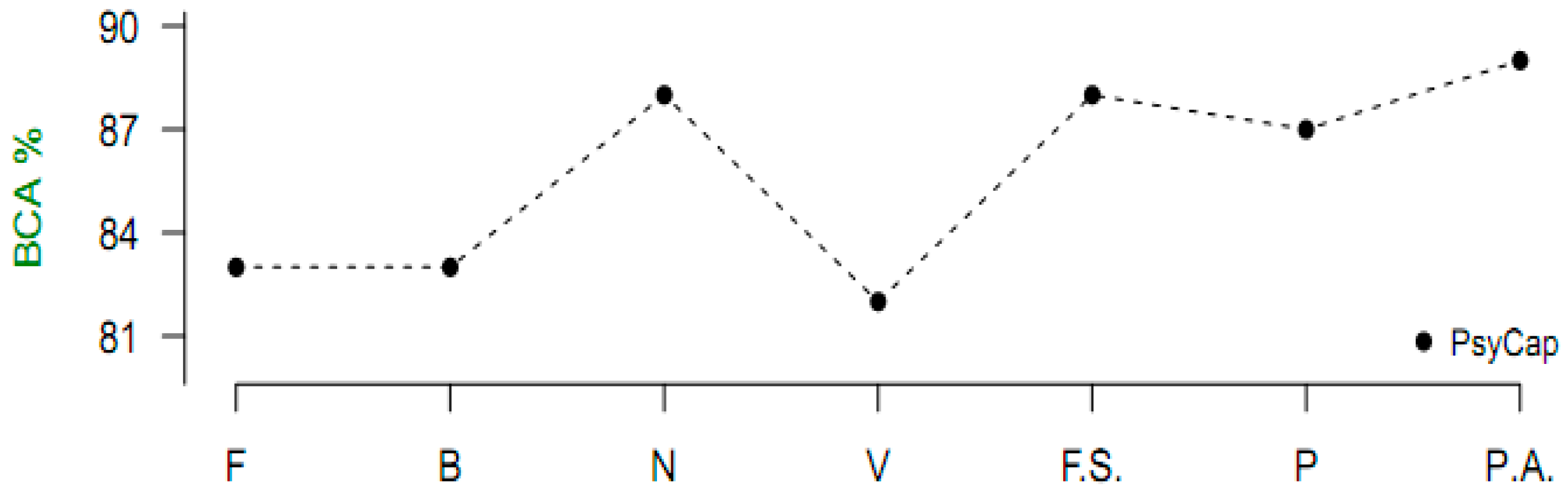
. The Table 5 indicates the predictive accuracy comparison of various ranking algorithms on the PsyCap dataset, while Table 6 reports results of predictive accuracies on the Diabetes dataset. Relatedly, Table 7 reports various predictive accuracies generated by each ranking algorithm on the Melanoma dataset, while Table 8 presents accuracy results on the Spam dataset. In Table 9, the predictive accuracies on the Cancer dataset for the various ranking algorithms are reported.

As could be observed in Table 5, Table 6, Table 7, Table 8 and Table 9, the variable subsets selected by the proposed algorithm performed competitively with the selection by existing algorithms.

4. Discussion

A predictive accuracy test was conducted in order to determine how well the variables selected by both existing algorithms and the proposed algorithm can predict the outcome variable $Y$ on the validation set. Output was determined as probabilities of the form $P(Y=1|X_i),$ where $X_i$ is the data value for each predictor, $i=1,\dots ,n$. The boundary used in making a decision was $0.5$. What the program typically did was that, if $P(Y=1|X_i)>0.5$ then $Y=1,$ otherwise $Y=0$. When this test was run on the different models generated by the various ranking algorithms, their respective predictive accuracies were obtained using Equation (6).

Figure 1 and Figure 2 represent graphically that variables selected by the proposed algorithm in all datasets produced higher predictive accuracies, except in one instance, compared with the selections by the existing algorithms. Therefore, the new algorithm can be said to be a good choice of filter variable ranking in machine learning classification.

Apart from selecting variable subsets that resulted in good model performance, another plus for the proposed algorithm over the existing algorithms is the way ranking values are presented to the user. As could be observed in Table 3, one of the ranking values in the diabetes dataset is a negative number. For quick insights into how much one predictor is more or less important than another, it would be better for all values to carry the same sign across the board. The Pearson’s is a correlation-based method, which means all ranking values produced will fall within the interval [−1,1]. In big data, where some datasets consist of a high number of features, say 100 and above, ranking the entire feature space within this interval may not give quick visual insights. The RR deployed in the proposed algorithm produces values within the range of 0 to infinity. This range seems more appropriate for representing ranking values when the feature space is large.

5. Conclusions

In the era of big data, where voluminous, high-dimensional data are constantly being generated from healthcare delivery activities, it is necessary to pay more attention to the problem of variable selection. The majority of the attributes that come with historical or daily data are usually not necessary in modeling. When such unimportant attributes are not eliminated before model construction, many metrics of model diagnostics, such as variance, deviance, degrees of freedom, and predictive accuracy, are negatively affected. Furthermore, machine learning algorithms train slower, and constructed models are over-fitted and more complex to interpret if irrelevant predictors are included. The ranking algorithm developed in this research, which performs competitively with some existing algorithms, will be a useful tool for dimensionality reduction in healthcare data to guard against these unwanted results in classification.

As could be observed in Figure 1 and Figure 2, this algorithm demonstrates that it is more appropriate for healthcare datasets than other domains. Better performance was recorded in the cancer, PsyCap, diabetes, and melanoma datasets compared with the spam e-mail dataset. The algorithm achieves a variable importance ranking by employing the statistical measure of risk ratio to evaluate the association between a predictor and the response. Predictors exhibiting a strong association with the class will be selected for classification, while those with a weak association will be excluded. The algorithm does not include a means of determining a threshold of which variables to include in a model. It is left to the discretion of the modeler to apply trial and error in adding or removing variables based on the ranking and performance of previous models. In future research, the algorithm should be extended to be able to determine a cut-off point of important variables algorithmically. Also, the possibility of implementing this algorithm in a way that makes it compatible with open-source languages, such as R, should be explored. As a candidate filter method, the algorithm is independent of any machine learning tool. It is meant to effect variable selection as a preprocessing activity, after which any modeling tool can be applied for model fitting proper. The algorithm is generic; thus, it can execute on any healthcare dataset, provided it is numeric with a dichotomous response.

References

1. Genuer, R.; Poggy, J.; Tuleau-Malot, C. Variable Selection Using Random Forests. Pattern Recognit. Lett. 2010, 31, 2225–2236. [Google Scholar] [CrossRef]
2. Tharwat, A. Classification Assessment Methods. Appl. Comput. Inf. 2018, in press. [Google Scholar] [CrossRef]
3. Lever, J.; Krzywinski, M.; Altman, N.S. Points of Significance: Classification Evaluation. Nat. Methods 2016, 13, 603–604. [Google Scholar] [CrossRef]
4. Schmidt, C.O.; Kohlmann, T. When to Use the Odds Ratio or the Relative Risk? Int. J. Public Health 2008, 53, 165–167. [Google Scholar] [CrossRef] [PubMed]
5. Last, A.; Wilson, S. Relative Risks and Odds Ratios: What’s the Difference? J. Fam. Pract. 2004, 53, 108. [Google Scholar]
6. Tamhane, A.R.; Westfall, A.O.; Burkholder, G.A.; Cutter, G.R. Prevalence Odds Ratio Versus Prevalence Ratio: Choice Comes with Consequences. Stat. Med. 2016, 35, 5730–5735. [Google Scholar] [CrossRef]
7. Rohde, J.M.; Dimcheff, D.E.; Blumberg, N.; Saint, S.; Langa, K.M. Health Care-Associated Infection after Red Blood Cell Transfusion: A Systematic Review and Meta-Analysis. J. Am. Med. Assoc. 2014, 311, 1317–1326. [Google Scholar] [CrossRef]
8. Capistrant, B.D.; Moon, J.R.; Glymour, M.M. Spousal Caregiving and Incident Hypertension. Am. J. Hypertens. 2012, 25, 437–443. [Google Scholar] [CrossRef]
9. Tseng, C. Diabetes and Risk of Prostate Cancer: A Study using the National Health Insurance. Diabetes Care 2011, 34, 616–621. [Google Scholar] [CrossRef]
10. Ditzler, G.; Polikar, R.; Rosen, G. A Bootstrap Based Neyman-Pearson Test for Identifying Variable Importance 2015. IEEE Trans. Neural Netw. Learn. Syst. 2015, 4, 880–886. [Google Scholar] [CrossRef]
11. Hwang, K.; Kim, D.; Lee, K.; Lee, C.; Park, S. Embedded Variable Selection Method Using Signomial Classification 2017. Ann. Oper. Res. 2017, 254, 89–109. [Google Scholar] [CrossRef]
12. Javed, K.; Babri, H.A.; Saeed, M. Impact of a Metric of Association Between two Variables on Performance of Filters for Binary Data. Neurocomputing 2014, 143, 248–260. [Google Scholar] [CrossRef]
13. Rodriguez-Galiano, V.F.; Luque-Espinar, J.A.; Chica-Olmo, M.; Mendes, M.P. Feature Selection Approaches for Predictive Modelling of Groundwater Nitrate Pollution: An Evaluation of Filters, Embedded and Wrapper Methods. Sci. Total Environ. 2018, 624, 661–672. [Google Scholar] [CrossRef] [PubMed]
14. Maldonado, S.; Weber, R. A Wrapper Method for Feature Selection Using Support Vector Machines. Inf. Sci. 2009, 179, 2208–2217. [Google Scholar] [CrossRef]
15. Chandrashekar, G.; Sahin, F. A Survey on Feature Selection Methods. Comput. Electr. Eng. 2014, 40, 16–28. [Google Scholar] [CrossRef]
16. R Core Team. R: A Language and Environment for Statistical Computing; R Foundation for Statistical Computing: Vienna, Austria, 2017; Available online: https://www.R-project.org/ (accessed on 11 December 2018).
17. Lumley, T. Leaps: Regression Subset Selection. R Package Version 3.0. 2017. Available online: https://CRAN.R-project.org/package=leaps (accessed on 12 December 2018).
18. Kuhn, M.; Wing, J.; Weston, S.; Williams, A.; Keefer, C.; Engelhardt, A.; Cooper, T.; Mayer, Z.; Benesty, M.; Lescarbeau, R.; et al. Caret: Classification and Regression Training, R Package Version 6.0-77. 2017. Available online: https://CRAN.R-project.org/package=caret (accessed on 12 December 2018).
19. Strobl, C.; Boulesteix, A.; Zeileis, A.; Hothorn, T. Bias in Random Forest Variable Importance Measures: Illustrations, Sources and a Solution 2002. BMC Bioinform. 2007, 8. [Google Scholar] [CrossRef] [PubMed]
20. Liaw, A.; Wiener, M. Classification and Regression by Randomforest. R News 2002, 2, 18–22. [Google Scholar]
21. Wang, H.; Yang, F.; Luo, Z. An Experimental study of the Intrinsic Stability of Random Forest Variable Importance Measures. BMC Bioinform. 2016, 17–60. [Google Scholar] [CrossRef] [PubMed]
22. Hur, J.; Ihm, S.; Park, Y. A Variable Impacts Measurement in Random Forest for Mobile Cloud Computing. Wirel. Commun. Mob. Comput. 2017, 2017, 1–18. [Google Scholar] [CrossRef]
23. Andrade, C. Understanding Relative Risk, Odds Ratio, and Related Terms: As Simple as it can Get 2015. J. Clin. Psychiatry 2015, 76, 857–861. [Google Scholar] [CrossRef] [PubMed]
24. Pandis, N. Risk Ratio Vs Odds Ratio: Statistics and Research Design. Am. J. Orthod. Dentofac. Orthop. 2012, 142, 890–891. [Google Scholar] [CrossRef]
25. McNutt, L.; Wu, C.; Xue, X.; Hafner, J.P. Estimating the Relative Risk in Cohort Studies and Clinical Trials of Common Outcomes 2003. Am. J. Epidemology 2003, 157, 940–943. [Google Scholar] [CrossRef]
26. Stoltzfus, J.C. Logistic Regression: A brief Primer. Acad. Emerg. Med. 2011, 18, 1099–1104. [Google Scholar] [CrossRef]
27. Liu, D.; Li, T.; Liang, D. Incorporating Logistic Regression to Decision-Theoretic Rough Sets for Classifications. Int. J. Approx. Reason. 2014, 55, 197–210. [Google Scholar] [CrossRef]
28. Sperandei, S. Lessons in Biostatistics: Understanding Logistic Regression Analysis. Biochem. Med. 2014, 24, 12–18. [Google Scholar] [CrossRef]
29. Breiman, L. Random Forests. Machine Learning. Sci. Res. 2001, 45, 5–32. [Google Scholar] [CrossRef]
30. Catena, S.; Colla, V.; Vannucci, M. A Hybrid Feature Selection Method for Classification Purposes. In Proceedings of the UKSim-AMSS, 8th European Modeling Symposium on Mathematical Modeling and Computer Simulation EMS2014, Pisa, Italy, 21–23 October 2014; IEEE Computer Society: Washington, DC, USA, 2014. [Google Scholar] [CrossRef]
31. Antunes, A.C.; Caetano, A.; Cunha, M.P. Reliability and Construct Validity of the Portuguese Version of the Psychological Capital Questionnaire. Psychol. Rep. 2017, 120, 520–536. [Google Scholar] [CrossRef]
32. Paek, S.; Schuckert, M.; Kim, T.T.; Lee, G. Why is Hospitality Employees’ Psychological Capital Important? The effects of Psychological Capital on Work Engagement and Employee Morale. Int. J. Hosp. Manag. 2015, 50, 9–26. [Google Scholar] [CrossRef]
33. Venables, W.N.; Ripley, B.D. Modern Applied Statistics with S, 4th ed.; Springer: New York, NY, USA, 2002; pp. 331–349. [Google Scholar]
34. Smith, J.W.; Everhart, J.E.; Dickson, W.C.; Knowler, W.C.; Johannes, R.S. Using the ADAP Learning Algorithm to Forecast the Onset of Diabetes Mellitus. In Proceedings of the Annual Symposium on Computer Application in Medical Care, Orlando, FL, USA, 7–11 November 1998; IEEE Computer Society Press: Washington, DC, USA, 1998. [Google Scholar]
35. Canty, A.; Ripley, B. boot: Bootstrap R (S-Plus) Functions. R Package Version 1.3-20. 2017. Available online: https://cran.r-project.org/web/packages/boot/boot.pdf (accessed on 7 March 2019).
36. Maindonald, J.H.; Braun, J.W. DAAG: Data Analysis and Graphics Data and Functions. R Package Version 1.22.1. 2019. Available online: https://CRAN.R-project.org/package=DAAG (accessed on 7 March 2019).
37. Chen, M.; Mao, S.; Liu, Y. Big data: A Survey. Mob. Netw. Appl. 2014, 19, 171–209. [Google Scholar] [CrossRef]
38. Pandey, A.; Jain, A. Comparative Analysis of Knn Algorithm Using Various Normalization Techniques. Int. J. Comp. Netw. Inf. Secur. 2017, 11, 36–42. [Google Scholar] [CrossRef]
39. Jain, S.; Shukla, S.; Wadhvani, R. Dynamic Selection of Normalization Techniques Using Data Complexity Measures. Expert Syst. Appl. 2018, 106, 252–262. [Google Scholar] [CrossRef]
40. Chapela, J.G. Things that Make Us different: Analysis of Deviance with Time-Use Data. J. Appl. Stat. 2013, 40, 1572–1585. [Google Scholar] [CrossRef]
41. Wang, Z.; Bovik, A.C. Mean Squared Error: Love it or Leave it? A New Look at Signal Fidelity Measures. IEEE Signal Process. Mag. 2009, 26, 98–117. [Google Scholar] [CrossRef]
Figure 1. Balanced classification accuracy (BCA) results of the ranking algorithms of the PsyCap dataset, where F: Forward selection; B: Backward elimination; N: Nvmax; V: varlmp; F.S.: Fisher score; P: Pearson’s correlation; P.A.: Proposed Algorithm.
Processes 07 00222 g001
Figure 2. BCA results of the ranking algorithms, where F: Forward selection; B: Backward elimination; N: Nvmax; V: varlmp; F.S.: Fisher score; P: Pearson’s correlation; P.A.: Proposed Algorithm.
Processes 07 00222 g002