Universal Relationships in Hyperbranched Polymer Architecture for Batch and Continuous Step Growth Polymerization of AB₂-Type Monomers

Abstract

Design and control of hyperbranched (HB) polymer architecture by way of reactor operation is key to a successful production of higher-valued HB polymers, and it is essential in order to clarify the fundamental structural characteristics formed in representative types of reactors. In this article, the irreversible step growth polymerization of AB₂ type monomer is investigated by a Monte Carlo simulation method, and the calculation was conducted for a batch and a continuous stirred-tank reactor (CSTR). In a CSTR, a highly branched core region consisting of units with large residence times is formed to give much more compact architecture, compared to batch polymerization. The universal relationships, unchanged by the conversion levels and/or the reactivity ratio, are found for the mean-square radius of gyration Rg², and the maximum span length L_MS. For batch polymerization, the g-ratio of Rg² of the HB molecule to that for a linear molecule conforms to that for the random branched polymers represented by the Zimm-Stockmayer equation. A single linear equation represents the relationship between Rg² and L_MS, both for batch and CSTR. Appropriate process control in combination with the chemical control of the reactivity of the second B-group promises to produce tailor-made HB polymer architecture.

1. Introduction

Hyperbranched (HB) polymers are specialty polymeric materials, possessing compact architecture, a vast number of end groups that can be functionalized, and specific space inside the molecule. A wide variety of potential applications have been and are being developed [1]. The HB polymers are macromolecules in between deterministic linear chains and dendrimer structures [2], and their properties are influenced significantly by their detailed branched architecture. The prediction and control of HB architecture is essential to produce higher quality polymers, which opens up a challenging field for the chemical engineers to develop novel production processes.

Basic chemical reaction engineering textbooks emphasize the importance in clarifying the fundamental chemical behavior in three representative reactor types; batch reactor, plug flow reactor (PFR), and continuous stirred-tank reactor (CSTR) [3]. Ideally, a PFR is equivalent to a batch reactor by changing the reaction time to the residence time. In this article, the differences in branched architecture formed in a batch reactor and a CSTR are considered.

For the synthesis of HB polymers consisting of tri-branched monomeric units, the two major chemical methods used are step growth polymerization of AB₂-type monomer and self-condensing vinyl polymerization (SCVP). The former is a classical synthetic route originally considered by Flory [4], but recent development in polymer chemistry has made it possible to change the chemical reactivity of the second B group freely [5], and has established the chemical control method for the branching frequency.

Figure 1 shows the reaction scheme of the step growth polymerization of AB₂ type monomer, considered in this article. In the figure, T is the terminal unit with both B’s being unreacted, L is the linearly incorporated unit with one of two B’s being reacted, and D is the dendritic unit in which both B’s have reacted. The reaction rate constant, k_T is for the reaction between an A group and a B group in T, while k_L is for the reaction between A and B in L. The reactivity of the second B group is represented by the reactivity ratio, r defined by:

r = k_L/k_T

(1)

The magnitude of r can be changed from 0 to infinity at will [5] by using appropriate chemical systems. For instance, it is possible to produce HB polymers with 100% degree of branching (DB, the exact definition will be given shortly), but the quasi-linear polymer can also be produced even with DB = 1, as illustrated earlier [5]. Process control in combination with chemical control is needed to synthesize well-designed HB polymers.

In this theoretical study, the branched molecular architecture is investigated by using a Monte Carlo (MC) simulation method proposed earlier for a batch reactor [6,7] and for a CSTR [8,9]. In the MC simulation, the structure of each HB polymer can be investigated, and any desired structural information could be extracted. Figure 2 shows an example of HB polymer generated in the present MC simulation for a CSTR. In Figure 2, FP means the focal point unit that possesses an unreacted A group. Note that in the ring-free model employed in this article, there is only one unit in a molecule that bears unreacted A group.

This article is aimed at establishing the most fundamental characteristics of HB polymers formed based on the ideal chemical kinetics, and the non-idealities, such as cyclization and shielding [10] are not considered. Both cyclization and shielding depend heavily on the 3D architecture, and it is of prime importance to establish the ideal architecture first. As for the cyclization, only one ring per molecule is allowed. Because smaller rings have a better chance of being formed [11], the effect on the global architecture of large polymers, which is of major interest in this article, may not be significant. On the other hand, the shielding effect depends on the crowding of the 3D architecture, and inferences on crowding could be obtained from the present type of structural investigation.

One of the most simple and fundamental information of the HB architecture is the degree of branching (DB). The DB of an HB polymer was originally defined by [12]:

$$DB=\frac{T+D}{P}=\frac{2D+1}{P}$$

(2)

where P is the degree of polymerization (total number of units in a polymer molecule), i.e., P = T + D + L. Note that every time the L-type unit is converted to D, the number of T units increases by one, and therefore, the relationship, T = D + 1 always holds true for any HB architecture, as long as the ring formation through the intramolecular reaction between the focal point A group and the unreacted B group in the same molecule is neglected.

When there are no L units, such as for the perfect dendron, DB = 1. With the definition given by Equation (2), however, DB cannot go down to 0 because linear polymer structure always possesses one T unit at its tail. To avoid this problem, at the same time, to make balanced comparison with the HB polymers synthesized via SCVP in which the focal point is always the L-type, the following definition for the DB was proposed [6].

$$DB=\{\begin{array}{cc}2D/\left(P-2\right)& \mathrm{when}\mathrm{FP}\mathrm{is}\mathrm{L},\mathrm{with}P>3\\ 2\left(D-1\right)/\left(P-3\right)& \mathrm{when}\mathrm{FP}\mathrm{is}\mathrm{D},\mathrm{with}P>3\\ 0& \mathrm{for}P\le 3\end{array},$$

(3)

where FP means the focal point. In this article, DB defined by Equation (3) is used. For the case of the HB polymer shown in Figure 2, P = 27, D = 10, and the FP is the D-type, the DB is calculated to be DB = (2)(9)/(24) = 0.75. Obviously, the DB of large polymers, i.e., with P >> 1, is given by $DB\cong 2D/P$, in either type of definition.

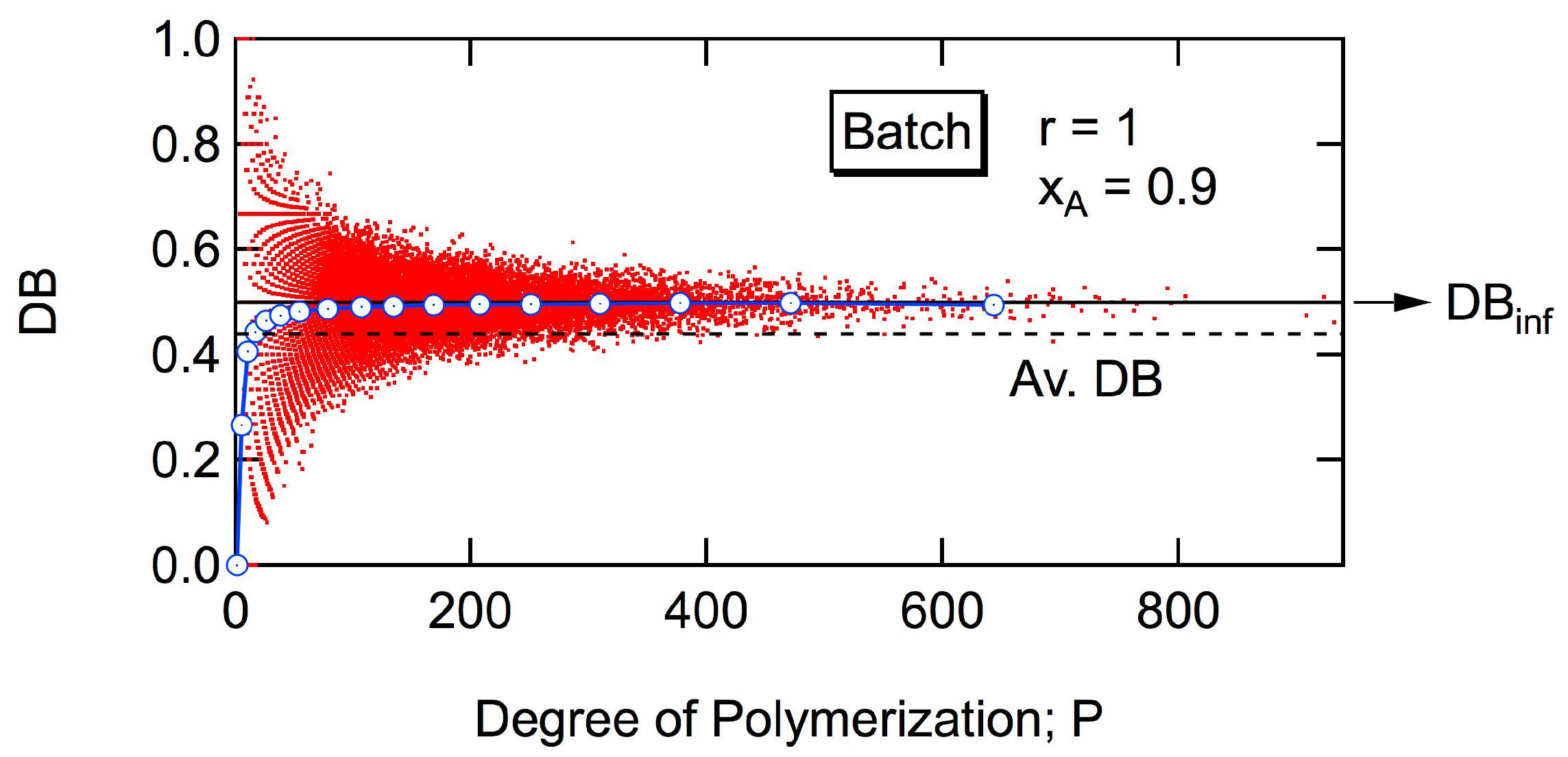
Figure 3 shows the relationship between the values of DB and P for batch polymerization with r = 1 when the conversion of A group is x_A = 0.9. The figure was prepared using the unpublished data obtained in the investigation reported earlier [6]. In the figure, each red dot shows a pair of values, DB and P, for each polymer molecule generated in the MC simulation. The circular symbols with a blue line show the average DB within each intervals of P, which shows the expected DB for the given P-value, $\overline{DB}(P)$. The DB-value converges to DB_inf, as the degree of polymerization P increases, i.e., for large polymers. On the other hand, the black broken line shows the magnitude of average DB of the whole reaction system. It is clearly shown that the values of DB are distributed around DB_inf, rather than the average DB of the whole system, and DB_inf is larger than the average DB. These characteristics hold true irrespective of the magnitude of reactivity ratio r, not only for a batch reactor [7] but also for a CSTR [8,9]. In this article, the HB architecture of large polymers, for which $\overline{DB}(P)$ has reached a constant value DB_inf, is investigated in detail, both for a batch reactor and a CSTR.

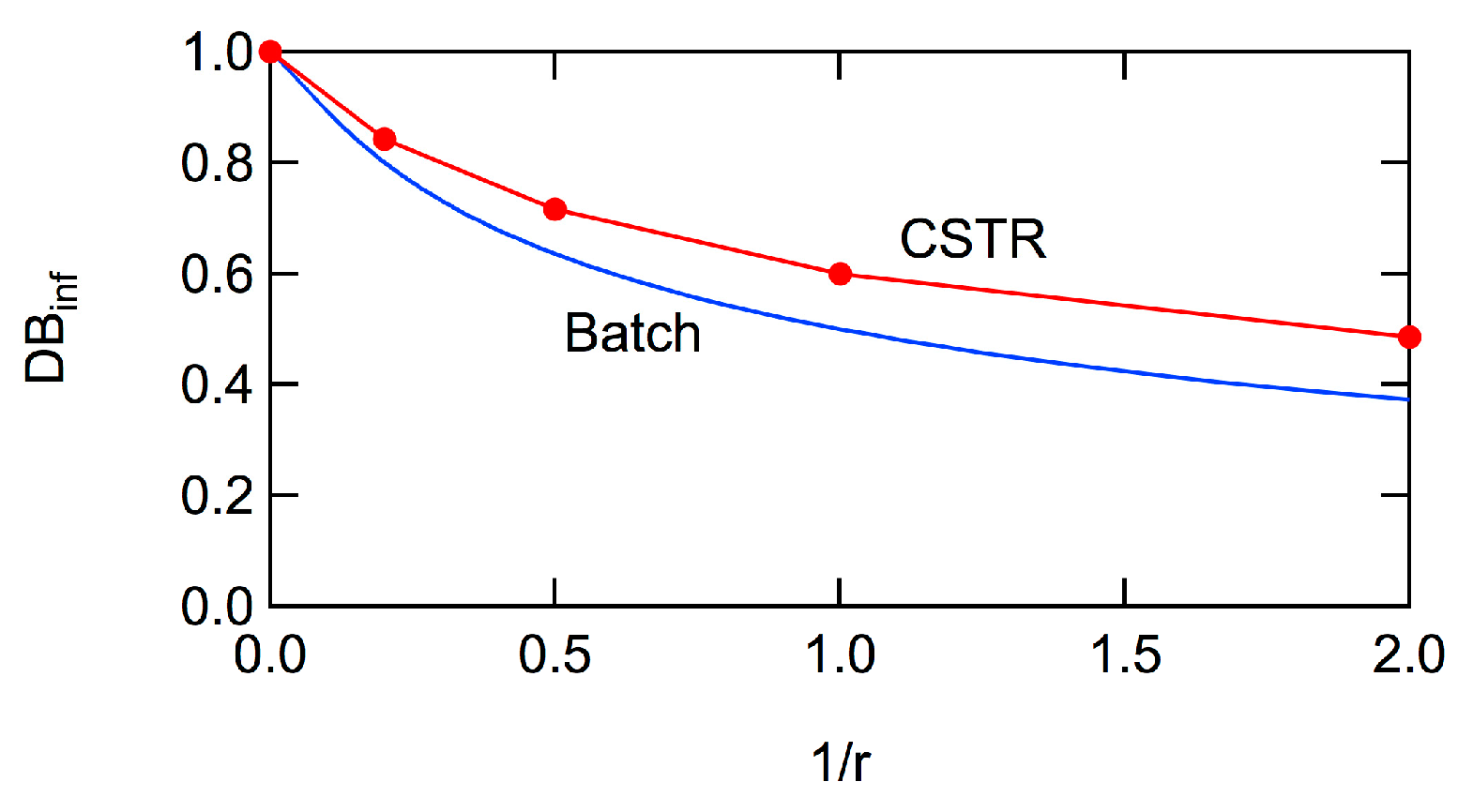
An interesting characteristic of DB_inf is that the magnitude of DB_inf is essentially kept constant, irrespective of the conversion level for a given reactivity ratio r, both for a batch reactor [6,7] and for a CSTR [8,9]. Note that the average DB of the whole reaction system increases with conversion, but DB_inf does not change. The value of DB_inf can be estimated by the reactivity ratio r, as shown in Figure 4. Obviously, DB_inf = 1 for the cases with r = ∞, both for batch and CSTR, but the value of DB_inf for a CSTR is always larger than that for a batch reactor, as long as r is finite. Incidentally, analytic relationship between DB_inf and r was established previously [6,7], and a smooth curve was drawn for batch polymerization in Figure 4. On the other hand, a general equation for a CSTR has not been reported, and five data points reported in the earlier publication [9] were plotted and connected.

Based on the structural information shown in Figure 2, it is possible to determine the 3D size, represented by the mean-square radius of gyration under the unperturbed condition, ${\langle s^2\rangle }_0$. One of the methods used to determine the value of ${\langle s^2\rangle }_0$ is the Wiener index (WI) [13]. The WI is related with ${\langle s^2\rangle }_0$ through the following relationship [14],

$$\frac{{\langle s^2\rangle }_0}{l^2}=\frac{WI}{N^2},$$

(4)

where l is the random walk segment length, and N is the number of such segments in the polymer molecule. N is related with P through N = P/u, where u is the number of monomeric units in a segment. In the previous investigation [6,7,8,9], as well as the present article, u = 1 is used. Define Rg² by the following equation,

$$R{g}^2=\frac{W{I}_{u=1}}{N^2},$$

(5)

where WI_{u = 1} is the value of WI when u = 1. Rg² is the value of ${\langle s^2\rangle }_0$ normalized by the squared monomer-unit length, and is proportional to ${\langle s^2\rangle }_0$, at least for large polymers, P >> 1. Note that Rg² is equal to the value of u${\langle s^2\rangle }_0$/l², which is unchanged irrespective of the magnitude of u, as long as the number N of steps is large enough.

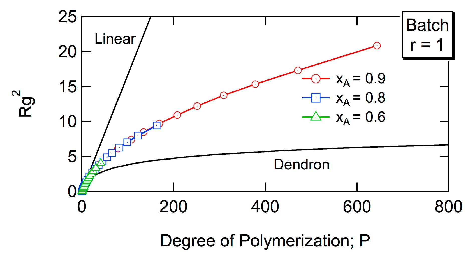
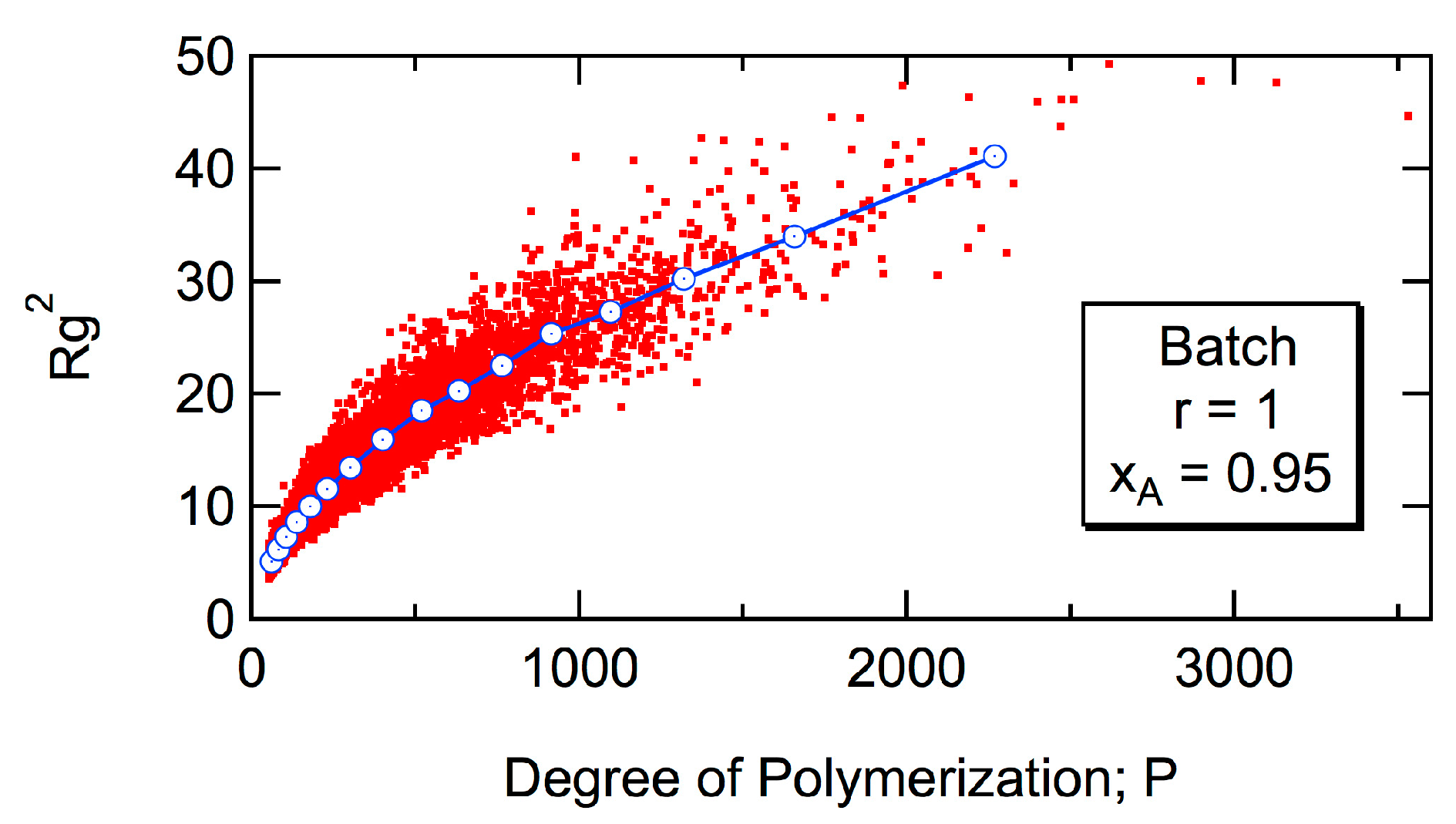
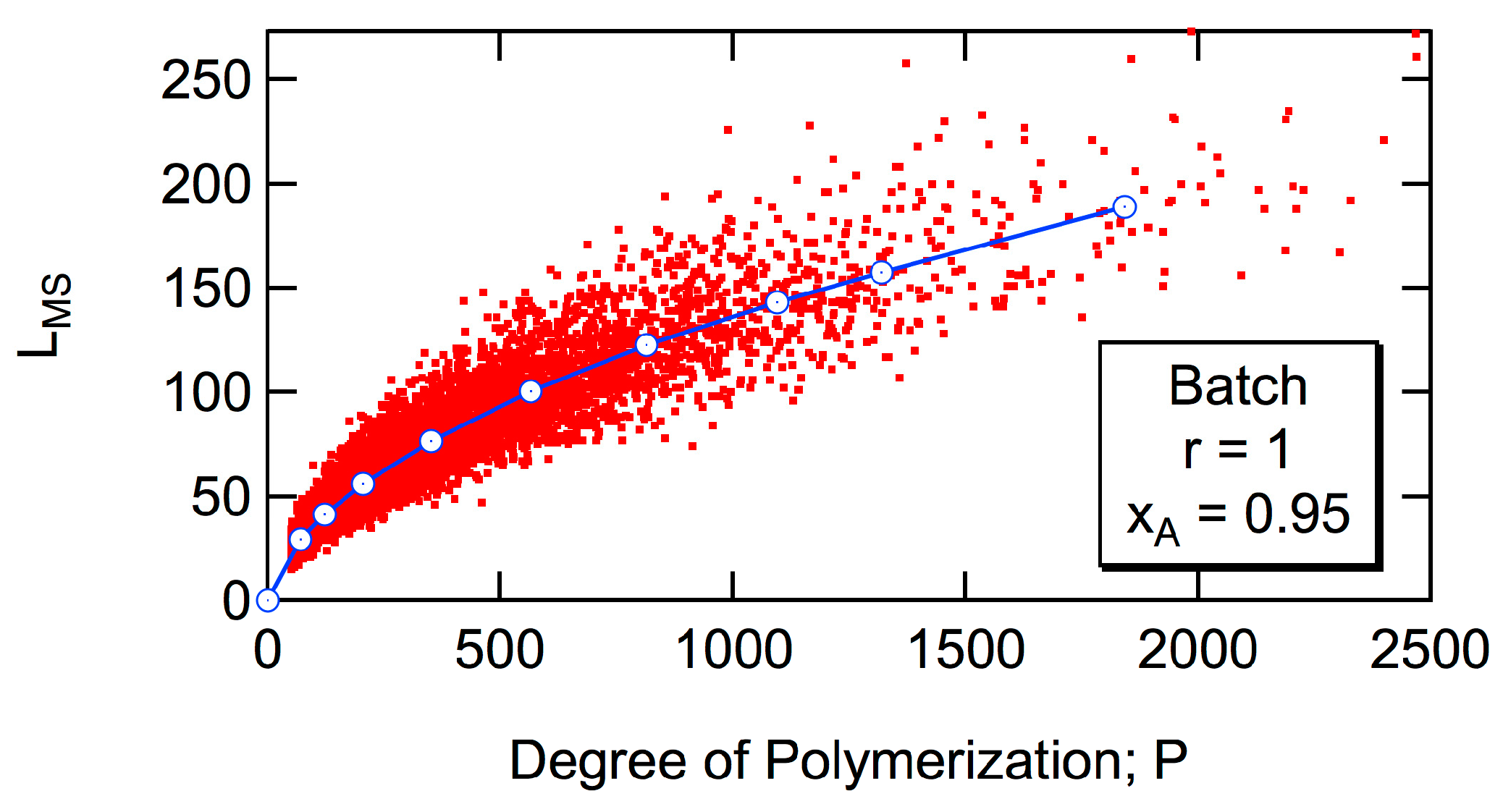
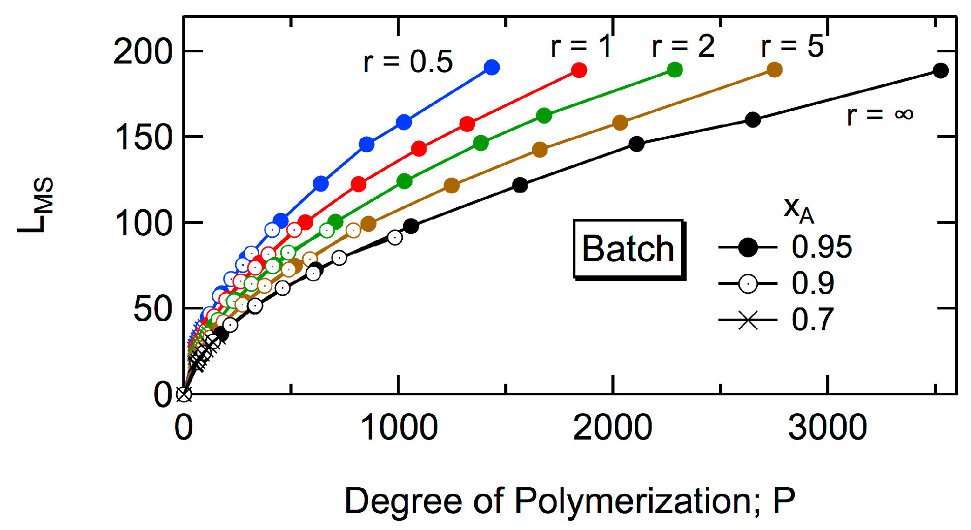
Figure 5 shows the expected Rg² of the polymer molecule whose degree of polymerization is P for batch polymerization with the reactivity ratio, r = 1. As shown in the figure, the relationship between Rg² and P does not change with the progress of conversion, x_A [6,7]. The curve moves to smaller Rg², as the reactivity ratio r is increased [7]. However, even with r = ∞ for which DB = 1, Rg² is much larger than that for the perfect dendron [7], which is shown by the black curve in Figure 4. 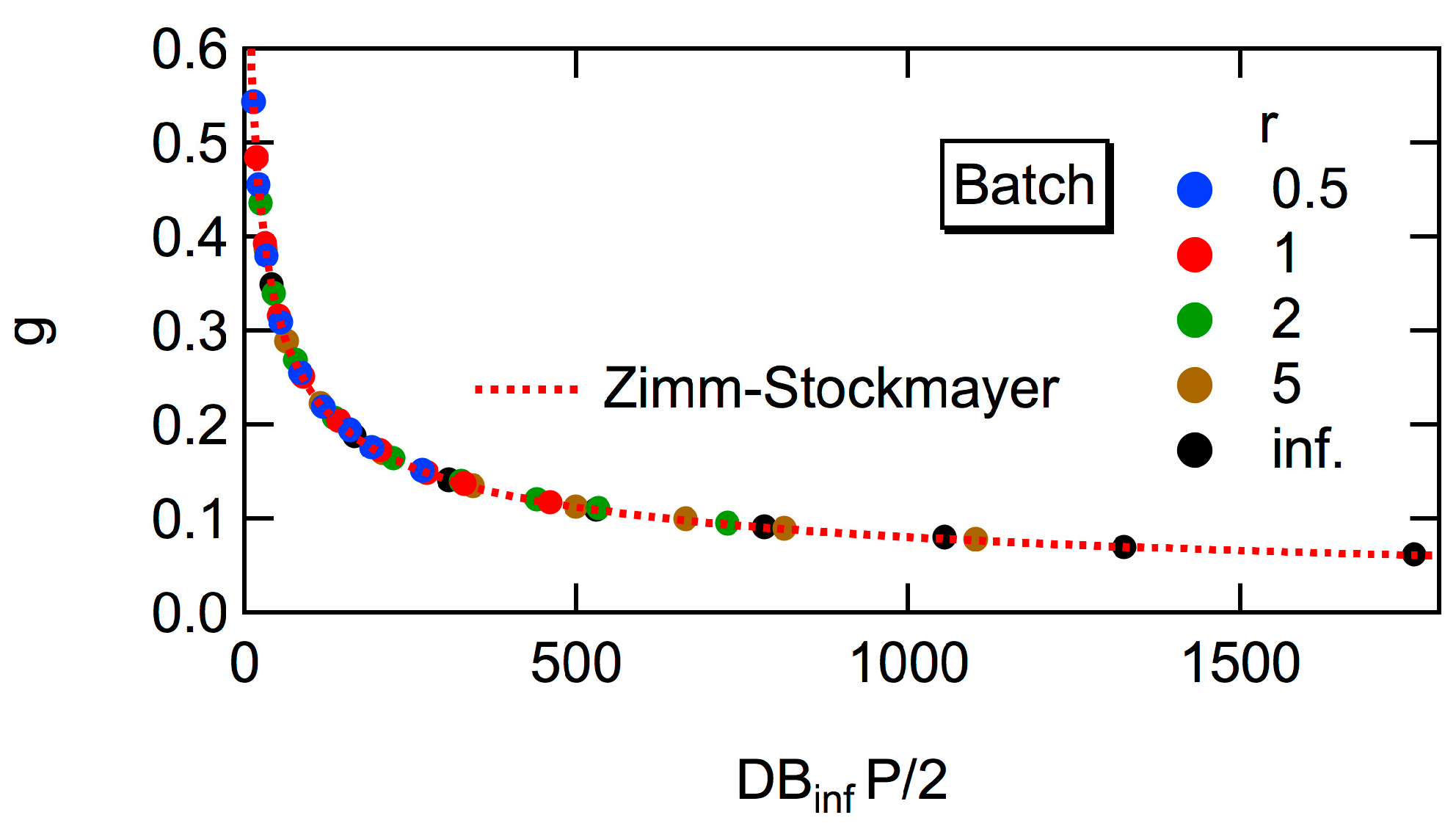For large polymers, the power law Rg² ~ P^0.5 is valid, irrespective of the magnitude of r [6,7]. The power exponent, 0.5 is the same as for the random branched polymers, represented by the Zimm-Stockmayer equation [15]. In this article, the universal relationship concerning Rg², that is independent of r, will be reported, and the relationship with the Zimm-Stockmayer equation will be discussed quantitatively.

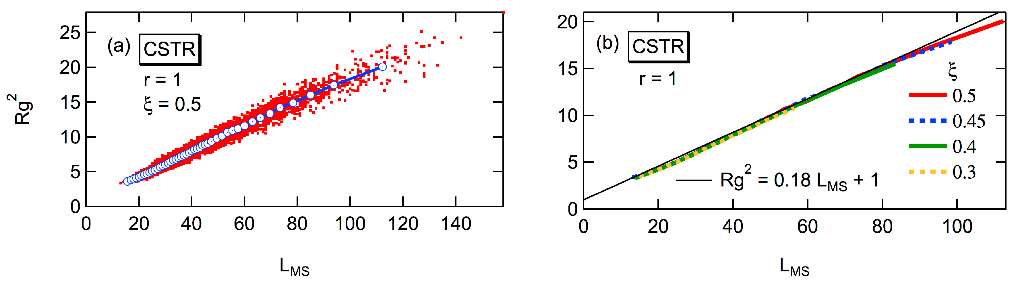
For a CSTR, the variance of Rg² for large polymers is quite large. It is not perfectly clear, but the relationship between Rg² and P does not change significantly, even when the steady state conversion level is changed [8,9]. 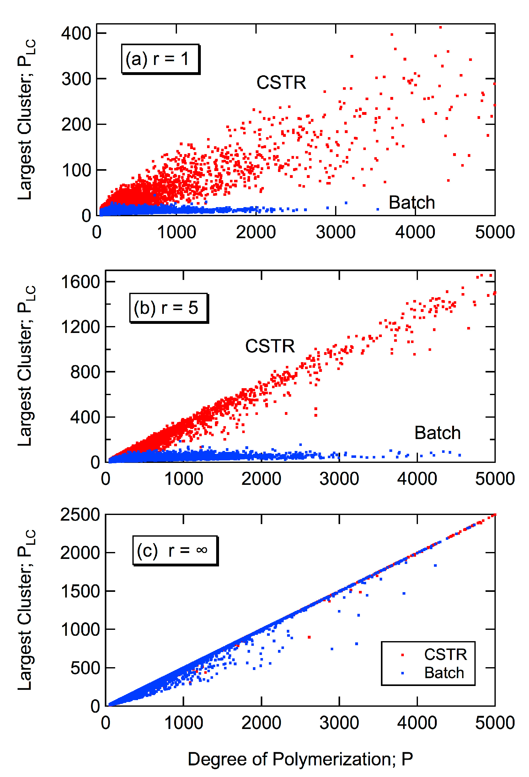It was clearly demonstrated that a CSTR produces polymers with much smaller Rg² compared with batch polymerization, even when the value of DB_inf is deliberately set to be the same for both types of reactors [8]. In this article, the reason for obtaining much more compact architecture in a CSTR is explored by considering the properties of the largest tri-branched cluster in a polymer molecule. The tri-branched clusters are shown by the group of D units surrounded by the red closed frames in Figure 2, and the largest cluster for this example consists of six units. Note that although the focal point unit is the D type, it is connected to only two other units and it is not considered as a tri-branched unit. A universal relationship concerning Rg², independent of the steady state conversion level, will also be reported for a CSTR.

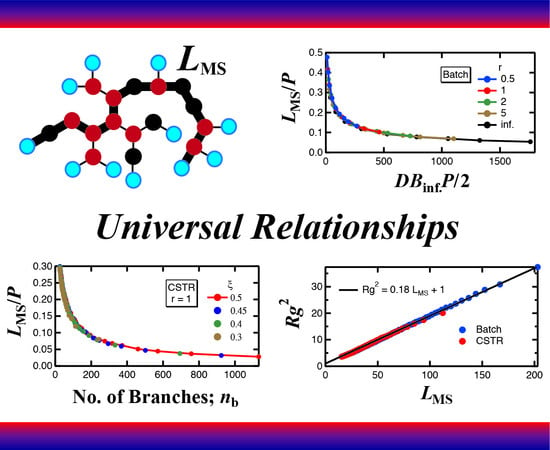
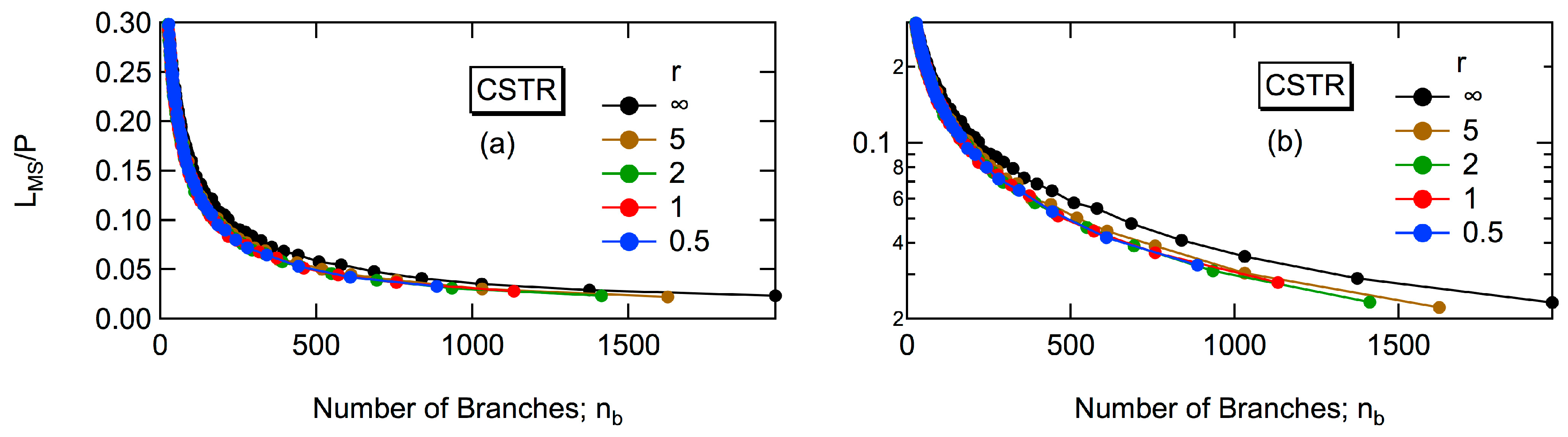
Another structural information investigated in this article is the maximum span length, L_MS. Here, the span length refers to the distance in the monomeric units [16], and L_MS is equivalent to the longest end-to-end distance [17]. In the case of HB polymer shown in Figure 2, L_MS = 12, which is the distance between the units with a star. There are two routes having L_MS = 12, starting from the unit with a star to the unit with star 1 or 2. Interesting universal relationships will be reported for the magnitude of L_MS.

In this article, the HB architecture formed in a batch and a CSTR is compared and discussed, by investigating the properties of the largest tri-branched cluster, and the magnitudes of Rg² and L_MS. For Rg² and L_MS, the universal relationships are sought. Note that the universal relationships reported so far for Rg² are with respect to the conversion level, and they change with the reactivity ratio r. In this article, further unification is explored.

2. Methods

The MC simulation method proposed earlier for batch polymerization [6,7], and that for a CSTR [8,9] were used to determine the branched architecture, as shown in Figure 2. This MC simulation method is based on the random sampling technique [18,19], and the polymer molecules were selected from the final product on a weight basis. The whole molecular architecture of each selected molecule was reconstructed by strictly following the history of branched structure formation. By generating a large number of polymer molecules in the simulation, the statistical properties were determined effectively. In the present investigation, the structural properties of large sized polymer molecules are highlighted, and 10⁴ polymer molecules with P > 50 were collected to determine statistically valid estimates. The reactivity ratios investigated were r = 0.5, 1, 2, 5, and ∞.

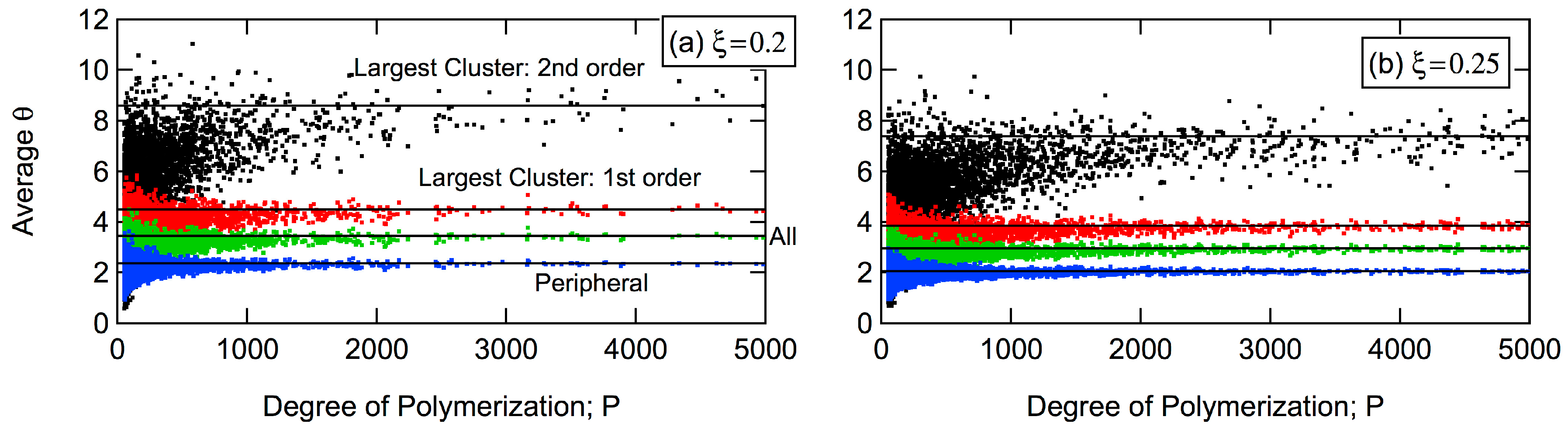
For a CSTR, the polymerization behavior at steady state is fully described by the reactivity ratio r and the dimensionless number ξ, sometimes referred to as the Damköhler number for the second order reaction, defined by:

$$\xi =k_{\mathrm{T}}{[\mathrm{A}]}_0\overline{t},$$

(6)

where [A]₀ is the initial concentration of A group, or equivalently, the initial monomer concentration, and $\overline{t}$ is the mean residence time [3]. The HB polymer shown in Figure 2 was generated for a CSTR with the condition, r = 2 and ξ = 0.35. The conversion of A group, x_A increases with ξ. To set the value of ξ corresponds to fixing the steady state conversion level, x_A.

For a CSTR, it was found that the weight-average molecular weight cannot reach the steady state for large $\overline{t}$ cases [8,9], and similar behavior was also reported for the SCVP [20,21] which is another route to synthesize HB polymers. The upper limit ξ-values above which the weight-average molecular weight cannot reach the steady state for a given reactivity ratio r was shown graphically in the earlier publication [9]. For example, the upper limit value of ξ is ξ_UL = 0.5 for r = 1, and ξ_UL = 0.25 for r = ∞. In the present investigation, the MC simulations were conducted for the cases with ξ ≤ ξ_UL.

The WI was calculated for each polymer molecule generated in the MC simulation, by setting up the distance matrix, {d_ij}, where d_ij is the distance in the number of monomeric units between the ith and jth unit. The WI when u = 1 is given by [13,14]:

$$W{I}_{u=1}=\frac{1}{2}{\displaystyle \sum _{i=1}^P{\displaystyle \sum _{j=1}^P{d}_{ij}}}.$$

(7)

The maximum span length, L_MS was determined by finding the largest value of d_ij in the distance matrix.

The statistical properties of various types of clusters in HB polymers were determined from the structural information, shown in Figure 2.

3. Results and Discussion

3.1. Largest Cluster of Tri-Branched Units

A CSTR produces much more compact HB polymers, compared with batch polymerization, as reported earlier [8,9]. First, the reason for this is explored by considering the size of the largest tri-branched cluster.

Figure 6 shows the relationship between the number of units P_LC belonging to the largest cluster and the number P of units in the polymer molecule (degree of polymerization). Each dot shows a set of values for each polymer molecule generated in the MC simulation. For a CSTR, the cases with ξ = ξ_UL are shown in the figure, while x_A = 0.95 for batch polymerization. General characteristics were the same for the other reaction conditions. For a CSTR, the largest cluster size P_LC increases with P, and a very large tri-branched cluster exists in a large polymer molecule. On the other hand, the size of the largest cluster does not increase significantly for batch polymerization, except for r = ∞. With r = ∞, all units other than the peripheral T units and a focal point are tri-branched units, and the largest cluster size is essentially proportional to P with P_LC ≈ 0.5P. Except for r = ∞, the existence of a large cluster of tri-branched units is an important characteristic of polymers formed in a CSTR, while a large number of small-sized clusters are formed in batch polymerization. It is reasonable to consider that the dimension is smaller for the HB polymers formed in a CSTR. The cases with r = ∞ will be discussed later, and consider the properties of various types of clusters for the cases with the reactivity ratio, r ≤ 5 first.

The largest tri-branched cluster consists of units whose residence times are different. In the case of the HB polymer shown in Figure 2, the largest tri-branched cluster consists of six units, and in general, the residence time of each unit is different. This kind of detailed information cannot be obtained in experiments, but can be determined in a straightforward manner in the present MC simulation method.

The average residence time of the units belonging to the largest tri-branched cluster is calculated, and is plotted as a red dot in Figure 7. In the same figure, the average residence time of all units in each polymer molecule, as well as that of the peripheral T units, is also shown. Here, the residence time is represented by the dimension residence time defined by [3]:

$$\theta =t/\overline{t}.$$

(8)

The average residence time approaches a constant value for all three types of units, as the molecular weight (MW) of the polymer increases. The constant value for each type of units decreases as the ξ-value, or equivalently, as the conversion level increases. At steady state for a given value of ξ, the convergent residence time shown by the black line is large for the largest cluster (red), which means that the largest cluster tends to be formed by connecting the units with larger residence times. On the other hand, the peripheral T units consist of units with smaller residence times. It would be reasonable to consider that there exists a gradient in the residence time distribution of units within an HB polymer. The core cluster of tri-branched region consists of units with large residence times, and the residence time of the units decreases toward the peripheral T type units. This tendency in the residence time distribution would be the reason for forming a compact architecture in a CSTR, compared with batch polymerization.

For the cases with r = ∞, a higher order tri-branched cluster is considered to differentiate the structure formed in batch and CSTR. Define the second order tri-branched cluster as a group of tri-branched units with all three bonds being connected to the tri-branched units, as shown by the regions enclosed by the blue broken curves in Figure 8. The largest group is named as the largest tri-branched cluster of the second order, and the number of units in such a group is represented by P_LC,2. In the present example shown in Figure 8, P_LC,2 = 2.

Figure 9 shows the relationship between P_LC,2 and P for batch and CSTR with r = ∞. For a CSTR, ξ = ξ_UL = 0.25, and x_A = 0.95 for batch polymerization. In the case of a CSTR, P_LC,2 increases with P, and therefore, a very large tri-branched cluster of the second order exists in a large polymer molecule. On the other hand, it does not increase significantly for batch polymerization, which means a large number of smaller-sized tri-branched clusters of the second order are formed. The smaller Rg² obtained for a CSTR could be understood from the significant differences in the magnitude of P_LC,2.

Figure 10 shows the average residence times for various types of units, as a function of P. Again, the average times of each type of units reach constant values for large polymers. The largest tri-branched cluster of the second order consists of units having very large residence times, while the units with smaller residence times tend to be the peripheral T units. There seems to exist a gradient in residence time distribution from the core region to the peripheral units. In a CSTR, a large core tri-branched cluster region is formed, which makes the architecture much more compact, compared with batch polymerization, also for the case with r = ∞.

In this section, it was shown that the branched architecture can be controlled by the residence time distribution. To form a core region is key to produce compact architecture. Obviously, the slow monomer addition method [22,23,24] is another way to form a core region to obtain compact architecture. On the other hand, if one needs looser structure, the core formation should be avoided. The structural control by using the tanks-in-series process was also discussed previously [25].

3.2. Radius of Gyration and Maximum Span Length

Both Rg² defined by Equation (5) and the maximum span length L_MS exemplified in Figure 2 are the characteristic factors describing the spatial size of an HB polymer. In this section, the universal relationships concerning Rg² and L_MS are explored both for a batch (Section 3.2.1) and a CSTR (Section 3.2.2).

3.2.1. Batch Polymerization

Figure 11 shows the MC simulation results for the relationship between Rg² and P with r = 1 at x_A = 0.95. Each red dot represents a set of Rg² and P, generated in the MC simulation. Note that the data were collected for P > 50 to clarify the statistical properties of large polymers, where $\overline{DB}(P)$ has reached a constant value, DB_inf. Blue circular symbols show the averages within ΔP fractions, and therefore, the blue line connecting these points represents the expected Rg²-value for a given P.

Figure 12 shows the expected Rg²-values that correspond to the blue curve in Figure 11 for various combinations of the reactivity ratio r and conversion x_A. The curve for the expected Rg²-value does not change with the conversion level x_A, and becomes smaller as the reactivity ratio r increases, as already reported earlier [6,7].

The contraction parameter, the ratio g of mean-square radius of gyration of the branched molecule to that for a linear molecule is given by [15]:

$$g={\frac{{\langle s^2\rangle }_{0,\mathrm{br}}}{{\langle s^2\rangle }_{0,\mathrm{lin}}}|}_{\mathrm{same}P}={\frac{R{g}_{\mathrm{br}}^2}{R{g}_{{}^{\mathrm{lin}}}^2}|}_{\mathrm{same}P}=\frac{6R{g}_{\mathrm{br}}^2}{P},$$

(9)

where the subscript “br” is for the branched polymer, and “lin” is for linear polymer. Note that Rg² is the defined by Equation (5), and therefore:

$$R{g}_{{}^{\mathrm{lin}}}^2=\frac{P}{6}.$$

(10)

Figure 13 shows the relationship between g and DB_infP/2. The value of DB_inf is a constant for a given reactivity ratio, and the value of DB_ifP/2 is equal to the average number ${\overline{n}}_{\mathrm{b}}$ of branch points per molecule for large polymers. Note that DB = 2D/P for large polymers, and ${\overline{n}}_{\mathrm{b}}$= DB_infP/2. Because the Rg²-value for a given P, as well as the magnitude of DB_inf, is the same at any conversion level x_A, the calculated results for x_A = 0.95 with various r’s are shown in Figure 13. All points fall on a single curve, showing a universal relationship, independent of x_A and r.

For the random branched polymers, the g-ratio is represented by the following Zimm-Stockmayer equation [15]:

$$g={\left[{\left(1+{\overline{n}}_{\mathrm{b}}/7\right)}^{\frac{1}{2}}+4{\overline{n}}_{\mathrm{b}}/9\pi \right]}^{-\frac{1}{2}}.$$

(11)

where ${\overline{n}}_{\mathrm{b}}$ is the average number of branch points per molecule.

Figure 14 shows the comparison with the Zimm-Stockmayer equation by using ${\overline{n}}_{\mathrm{b}}=D{B}_{\inf }P/2$, which shows an excellent fit. It is suggested that the HB architecture formed in a batch polymerization is random branch, irrespective of the magnitude of reactivity ratio, r. In batch polymerization, the probability that a randomly selected unit from the final product is the D type unit is the same for all units [6,7], and therefore, it is reasonable to obtain HB polymers with random branched architecture. On the other hand, in the case of a CSTR, the probability for a randomly selected unit from the final product being the D type unit is larger for the units with longer residence time, leading to a nonrandom branched architecture, as discussed in the previous section.

The value of DB_inf for a given r can be calculated analytically [6,7], and Figure 4 shows the calculated results graphically. Therefore, the value of Rg² can be determined by using Equation (11) in a straightforward manner, without conducting the MC simulation, for any combination of r and x_A.

Next, consider the maximum span length, L_MS. Figure 15 shows the MC simulation results for the relationship between L_MS and P with r = 1 and x_A = 0.95 for batch polymerization. Each red dot represents a set of L_MS and P, generated in the MC simulation. Blue circular symbols show the averages within ΔP fractions, and the blue line connecting these points represents the expected L_MS-value for a given P.

Figure 16 shows the expected L_MS-value for a given P, corresponding to the blue curve in Figure 15, for various combinations of the reactivity ratio r and conversion x_A. The curve for the expected L_MS-value does not change with the conversion level x_A, and is a function of the reactivity ratio r. The qualitative tendency is quite similar to Rg².

Figure 17 shows the expected value of L_MS/P for a given DB_infP/2. Because the L_MS-value for a given P, as well as the magnitude of DB_inf, is the same at any conversion level x_A, the calculated results for x_A = 0.95 with various r’s are shown in Figure 17. Note that the value of DB_infP/2 is equal to the average number of branch points per molecule for large polymers. All data points fall nicely on the same universal curve, as in the case of Rg².

Both Rg² and L_MS show a similar universal relationship, as shown in Figure 13 and Figure 17. Now, consider the relationship between Rg² and L_MS.

Figure 18a shows the relationship between Rg² and L_MS for r = 1 and x_A = 0.95, which shows a linear relationship. The blue line with circular symbols shows the expected Rg² for a given L_MS.

Figure 18b shows the expected Rg² at various conversion levels for r = 1. The plotted points shown by the blue circular symbols are the same as those in Figure 18a. The relationship is essentially unchanged by the conversion level, and the relationship fits reasonably well with:

$$R{g}^2=0.18L_{\mathrm{MS}}+1.$$

(12)

Figure 19 shows the expected Rg² for a given L_MS, for various combinations of x_A and r. A linear relationship seems to hold for any value of r. The black straight line shows the linear relationship given by Equation (12). Although a slight discrepancy is observed in the cases of r = 5 and ∞ for large polymers, the data points are well correlated with Equation (12). Equation (12) is the universal relationship between Rg² and L_MS, applicable to any combination of r and x_A in batch polymerization.

For the SCVP, the relationship, Rg² = 0.18 L_MS + 0.6 was reported both for a batch and a CSTR [26]. The proportional coefficient, 0.18 is the same as Equation (12), and the constant term is very close.

For linear polymers, L_MS is equal to P, and the following equation is valid for large polymers:

$$R{g}^2=L_{\mathrm{MS}}/6\cong 0.167L_{\mathrm{MS}}.$$

(13)

Note that Rg² is the mean-square radius of gyration when each monomeric unit is considered as the random walk segment.

In the case of linear polymers, there is no contribution to Rg² other than its own chain with P = L_MS. In the HB polymers, the chains other than the largest span chain can make a contribution to increase the Rg²-value. The increase in the coefficient from 0.167 to 0.18 could be considered as showing the degree of contribution from the other chains to the magnitude of Rg².

For the perfect dendrons, on the other hand, the numerical calculation results are shown in Figure 20, and the relationship for large L_MS-values is given by:

$$R{g}^2=0.5L_{\mathrm{MS}}-2.$$

(14)

The proportionality coefficient changes from 0.167 for linear polymers to 0.5 for perfect dendrons, and the HB polymers comes in between these two extremes. The value of 0.18 for the HP polymers is closer to linear polymers, rather than that for perfect dendrons, which shows that the magnitude of Rg² is still mainly determined by the maximum span chain, and the contribution of the other chains is not very significant. The exact physical meaning of the magnitude of coefficient is still an open question. However, the linear relationship found here is of great interest.

For batch polymerization, the value of Rg² can be determined analytically without MC simulation, as discussed earlier. By using Equation (12), the magnitude of L_MS can also be estimated in a straightforward manner, without relying on the MC simulation.

3.2.2. CSTR

In this section, basic characteristics of Rg² and L_MS are considered, as was done in the previous section. For a CSTR, however, the variance of Rg² for large polymer is quite large [8,9], and it is difficult to determine the statistically valid expected Rg²-values for large polymers. Inspired by the universal curve shown in Figure 13, the value of g-ratio defined by Equation (9) is plotted with respect to the number of branch points in a polymer molecule, n_b. Figure 21a shows the case with r = 1 at ξ = 0.5. In the figure, each red dot indicates a set of values for the polymer molecule generated in the MC simulation. With this type of plot, the variance of g for large polymers is rather small, and it is straightforward to determine the expected g-ratio for a given n_b, shown by the blue curve with circular symbols.

Figure 21b shows the expected g-ratio at various values of ξ for the case with r = 1. The data points fall on a single curve irrespective of the values of ξ, i.e., at any steady state conversion level. The universal relationship between g and n_b, unchanged by ξ, is confirmed also for the other r cases, as shown in Figure S1 of Supplementary Materials.

Figure 22 shows how the universal curves, shown in Figure 21b and Figure S1, change with the reactivity ratio r. Because the relationship does not change with ξ for a given r, the expected g-values at ξ = ξ_UL are shown in Figure 22. In order to magnify the small differences for smaller g-values, the logarithmic scale plot was used for Figure 22b. Slight differences among curves are observed, and the expected g-ratio is considered a very weak function of r. In particular, the change for r < 5 is not very significant.

In Figure 22, the g-ratio for the random branched polymers represented by the Zimm-Stockmayer equation, Equation (11), is also shown by the red broken curve. It is clearly shown that the HB architecture formed in a CSTR is much more compact than for the random branched polymers, i.e., for the HB polymers synthesized in a batch reactor.

Next, consider the maximum span length, L_MS for the HB polymers formed in a CSTR. Figure 23a shows the relationship between the weight fraction of the maximum span chain L_MS/P and n_b for r = 1 with ξ = 0.5. Each red dot shows the individual data point, and the blue curve with circular symbols shows the expected value of L_MS/P for a given n_b. Figure 23b shows the expected L_MS/P for various values of ξ, i.e., for different conversion levels at steady state. The expected values of L_MS/P do not change with ξ, and another universal relationship is found. The universal relationship between L_MS/P and n_b, unchanged by ξ, is confirmed also for the other r cases, as shown in Figure S2 of Supplementary Materials.

Figure 24 shows how the universal curve changes with the reactivity ratio r. Again, the relationship at ξ_UL is shown for each reactivity ratio. Figure 24a is the normal scale plot, which shows the differences among the curves are rather small. To enlarge the differences for smaller L_MS/P-values, the logarithmic plot is used for the y-axis of Figure 24b, and it is shown that up to r = 5, the differences are rather small, but the curve with r = ∞ shows slightly larger L_MS/P-values. Similarly with the g-ratio for a CSTR, the value of L_MS/P is a very weak function of the reactivity ratio r.

Finally, consider the relationship between Rg² and L_MS, as was done for batch polymerization in Figure 18 and Figure 19, which showed a universal relationship, represented by Rg² = 0.18L_MS + 1.

Figure 25a shows the relationship between Rg² and L_MS for HB polymers formed in a CSTR with r = 1 and ξ = 0.5, which shows a linear relationship. Figure 25b shows the expected Rg² at various ξ-values for r = 1. The relationship is essentially unchanged by the steady-state conversion level. The black line represents the relationship given by Equation (11). Although a slight deviation is observed for large values of L_MS, overall agreement is satisfactory. Compared with Figure 18, the absolute values of Rg² and L_MS are smaller for the case of CSTR, because of much more compact architecture formed in a CSTR.

The expected Rg²-values for various combinations of ξ and r are shown in Figure S3 of Supplementary Materials. The universal relationship, represented by Equation (12), correlates reasonably well, irrespective of the magnitude of ξ and r, and Equation (12) could be considered as a universal relationship that holds for both batch and CSTR. Even though a CSTR leads to form much more compact HB polymers, such difference in branched structure does not affect the relationship, Rg² = 0.18L_MS + 1.

The physical meaning of the magnitude of proportionality coefficient is not clear at the present stage, however, the proportionality coefficient, 0.18 is closer to that for linear polymers (0.167), rather than for the perfect dendron (0.5). The perfect dendron suffers from the Malthusian packing paradox [27] and cannot fit in the 3D space. Closer value to that for linear polymers may imply that the structure does not suffer from the space dimensionality. In fact, the Rg²-value of the HB polymers formed with r = ∞ in a CSTR is still much larger than that for the perfect dendron [9].

For a CSTR, the value of DB_inf for a given r is represented graphically in Figure 4. At least approximately for large polymers, n_b is estimated to be n_b = DB_infP/2. Therefore, the magnitude of Rg² can be estimated from Figure 22, and the value of L_MS could also be estimated by using the relationship, Rg² = 0.18L_MS + 1.

Obviously, various non-idealities, notably the size and structural dependent reaction kinetics, may need to be accounted for in a real system. The information concerning the 3D architecture obtained for the present ideal condition could be used as a starting point for the discussion of such non-ideal reaction kinetics, and the present results would provide a basis for the development of more realistic models for the HB polymer formation.

4. Conclusions

The HB polymer architecture formed in a batch and a CSTR is investigated in detail, by using the MC simulation method, proposed earlier [6,7,8,9]. In a CSTR, a highly branched core region consisting of units with large residence times is formed to give much more compact architecture, compared with batch polymerization for large polymers. The branched architecture can be controlled by the residence time distribution.

For batch polymerization, the g-ratio, as well as L_MS/P, shows a universal relationship with the average number of branches per molecule, which is independent of conversion x_A and reactivity ratio r. The g-ratio follows the relationship given by the Zimm-Stockmayer equation [15], which shows that the random branched structure is formed in batch polymerization.

For a CSTR, the g-ratio, as well as L_MS/P, follows a universal relationship with the number of branches in a polymer molecule, and the relationship is independent of ξ, but is a very weak function of r.

It was found that the Rg² is linearly correlated with L_MS, represented by Rg² = 0.18L_MS + 1, both for a batch and a CSTR, irrespective of the conversion level and reactivity ratio. The coefficient, 0.18 is essentially the same as for an SCVP [26], and could be considered as a general characteristic of HB polymer architecture. The coefficient is 0.167 for linear polymers, and is 0.5 for perfect dendrons. The physical meaning of the coefficient is still not clear, but the value of 0.18 is closer to that for the linear polymers, rather than the perfect dendron that cannot fit in the 3D space because of the Malthusian packing paradox.

The HB polymer architecture can be controlled by the residence time distribution. Appropriate process control in combination with the chemical control of the reactivity of the second B-group will make it possible to produce HB polymers with well-controlled molecular architecture.

References

1. Zheng, Y.; Li, S.; Weng, Z.; Gao, C. Hyperbranched polymers: Advances from synthesis to application. Chem. Soc. Rev. 2015, 44, 4091–4130. [Google Scholar] [CrossRef] [PubMed]
2. Lederer, A.; Burchard, W. Hyperbranched Polymers: Macromolecules in between Deterministic Linear Chains and Dendrimer Structure; The Royal Society of Chemistry: Cambridge, UK, 2015. [Google Scholar]
3. Levenspiel, O. Chemical Reaction Engineering, 2nd ed.; John Wiley & Sons: New York, NY, USA, 1972. [Google Scholar]
4. Flory, P.J. Molecular size distribution in three dimensional polymers. VI. Branched polymers containing A-R-Bf-1 type units. J. Am. Chem. Soc. 1952, 74, 2718–2723. [Google Scholar] [CrossRef]
5. Segawa, Y.; Higashihara, T.; Ueda, M. Synthesis of hyperbranched polymers with controlled structure. Polym. Chem. 2013, 4, 1746–1759. [Google Scholar] [CrossRef]
6. Tobita, H. Universality in branching frequrncies and molecular dimensions during hyperbranched polymer formation: 1. step polymerization of AB2 type monomer with equal reactivity. Macromol. Theory Simul. 2016, 25, 116–122. [Google Scholar] [CrossRef]
7. Tobita, H. Universality in branching frequrncies and molecular dimensions during hyperbranched polymer formation: 2. step polymerization of AB2 type monomer with different reactivity for the second B group. Macromol. Theory Simul. 2016, 25, 123–133. [Google Scholar] [CrossRef]
8. Tobita, H. Hyperbranched polymers formed through irreversible step polymerization of AB2 type monomer in a continuous flow stirred-tank reactor (CSTR). Macromol. Theory Simul. 2017, 26, 1600078. [Google Scholar] [CrossRef]
9. Tobita, H. Hyperbranched polymers formed through irreversible step polymerization of AB2 type monomer with substitution effect in a continuous flow stirred-tank reactor (CSTR). Macromol. Theory Simul. 2017, 26, 1700020. [Google Scholar] [CrossRef]
10. Kryven, I.; Iedema, P.D. Predicting multidimensional distributive properties of hyperbranched polymer resulting from AB2 polymerization with substitution, cyclization and shielding. Polymer 2013, 54, 3472–3484. [Google Scholar] [CrossRef]
11. Jacobson, H.; Stockmayer, W.H. Intramolecular reaction in polycondensations. I. The theory of linear systems. J. Chem. Phys. 1950, 18, 1600–1606. [Google Scholar] [CrossRef]
12. Hawker, C.J.; Lee, R.; Fréchet, M.J. One-step synthesis of hyperbranched dendritic polyesters. J. Am. Chem. Soc. 1991, 113, 4583–4588. [Google Scholar] [CrossRef]
13. Wiener, H. Structural determination of paraffin boiling points. J. Am. Chem. Soc. 1947, 69, 17–20. [Google Scholar] [CrossRef]
14. Nitta, K. A topological approach to statistics and dynamics of chain molecules. J. Chem. Phys. 1994, 101, 4222–4228. [Google Scholar] [CrossRef]
15. Zimm, B.H.; Stockmayer, W.H. The dimensions of chain molecules containing branches and rings. J. Chem. Phys. 1949, 17, 1301–1314. [Google Scholar] [CrossRef]
16. Versluis, C.; Souren, F.; Nijenhuis, A. Span-length distributions of star-branched polymers. Macromol. Theory Simul. 2002, 11, 969–974. [Google Scholar] [CrossRef]
17. Iedema, P.D.; Hoefsloot, H.C.J. Synthesis of branched polymer architectures from molecular weight and branching distributions for radical polymerization with long-chain branching, accounting for topology-controlled random scission. Macromol. Theory Simul. 2001, 10, 855–869. [Google Scholar] [CrossRef]
18. Tobita, H. Random sampling technique to predict the molecular weight distribution in nonlinear polymerization. Macromol. Theory Simul. 1996, 5, 1167–1194. [Google Scholar] [CrossRef]
19. Tobita, H. Polymerization Processes, 1. Fundamentals. In Ullmann’s Encyclopedia of Industry Chemistry; Elvers, B., Ed.; Wiley: Weinheim, Germany, 2015. [Google Scholar] [CrossRef]
20. Buren, B.D.; Zhao, Y.R.; Puskas, J.E.; McAuley, K.B. Predicting average molecular weight and branching level for self-condensing vinyl copolymerization. Macromol. React. Eng. 2018, 12, 1700074. [Google Scholar] [CrossRef]
21. Tobita, H. Hyperbranched polymers formed through self-condensing vinyl polymerization in a continuous stirred-tank reactor (CSTR): 1. molecular weight distribution. Macromol. Theory Simul. 2018, 27, 1800027. [Google Scholar] [CrossRef]
22. Hölter, D.; Frey, H. Degree of branching in hyperbranched polymers. 2. Enhancement of the DB: Scope and limitation. Acta Polym. 1997, 48, 298–309. [Google Scholar] [CrossRef]
23. Hanselmann, R.; Hölter, D.; Frey, H. Hyperbranched polymers prepared via the core-dilution/slow addition technique: Computer simulation of molecular weight distribution and degree of branching. Macromolecules 1998, 31, 3790–3801. [Google Scholar] [CrossRef]
24. Cook, A.B.; Barbey, R.; Burns, J.A.; Perrier, S. Hyperbranched polymers with high degrees of branching and low polydispersity values: Pushing the limits of thiol-yne chemistry. Macromolecules 2016, 49, 1296–1304. [Google Scholar] [CrossRef]
25. Tobita, H. Model-based reactor design to control hyperbranched polymer architecture. Macromol. React. Eng. 2018, 12, 1700065. [Google Scholar] [CrossRef]
26. Tobita, H. Detailed structural analysis of the hyperbranched polymers formed in self-condensing vinyl polymerization. Macromol. Theory Simul. 2019, 28, 1800061. [Google Scholar] [CrossRef]
27. Gordon, M.; Ross-Murphy, S.B. The structure and properties of molecular trees and networks. Pure Appl. Chem. 1975, 43, 1–26. [Google Scholar] [CrossRef]
Figure 1. Reaction scheme for the step growth polymerization of AB2 type monomer.
Processes 07 00220 g001
Figure 2. Schematic representation of a hyperbranched (HB) polymer molecule generated in the present Monte Carlo (MC) simulation for a continuous stirred-tank reactor (CSTR). The tri-branched clusters are shown by the red closed curves, and the T units with a star show the end units for the maximum span length.
Processes 07 00220 g002
Figure 3. Relationship between degree of branching (DB) and P for batch polymerization with r = 1 at the conversion level of A, xA = 0.9. Similar figures can be found in the earlier publications for a batch reactor [6,7] and for a CSTR [8,9].
Processes 07 00220 g003
Figure 4. Relationship between DBinf and r for batch and CSTR. Data points were taken from the earlier publication [9].
Processes 07 00220 g004
Figure 5. Expected Rg2-values of the polymers having P for batch polymerization with r = 1. Redrawn by using the data reported earlier [6].
Processes 07 00220 g005
Figure 6. Relationship between the number PLC of units belonging to the largest cluster and the degree of polymerization P. (a) r = 1; ξ = 0.5 for CSTR, and xA = 0.95 for batch. (b) r = 5; ξ = 0.306 for CSTR, and xA = 0.95 for batch. (c) r = ∞; ξ = 0.25 for CSTR, and xA = 0.95 for batch.
Processes 07 00220 g006
Figure 7. Average residence time of the units in the largest tri-branched cluster (red), of all units (green), and of the peripheral T units (blue) in each polymer molecule for the cases with r = 1. (a) ξ = 0.4, and (b) ξ = 0.5.
Processes 07 00220 g007
Figure 8. Example of the hyperbranched polymer architecture generated in the present MC simulation for a CSTR with r = ∞ and ξ = 0.2. The tri-branched clusters of the first order are represented by the groups enclosed by the red broken curves, while the tri-branched clusters of the second order by the blue broken curves. For this polymer, P = 43, D = 21, and DB = 1.
Processes 07 00220 g008
Figure 9. Relationship between the number PLC,2 of units belonging to the largest cluster of the second order and the degree of polymerization P, for a batch and a CSTR with r = ∞. ξ = 0.25 for CSTR, and xA = 0.95 for batch.
Processes 07 00220 g009
Figure 10. Average residence time of the units in the largest tri-branched cluster of the second order (black dots), of the units in the largest tri-branched cluster of the first order (red), of all units (green), and of the peripheral T units (blue) for the cases with r = ∞. (a) ξ = 0.2, and (b) ξ = 0.25.
Processes 07 00220 g010
Figure 11. Relationship between Rg2 and P with r = 1 and xA = 0.95 for batch polymerization.
Processes 07 00220 g011
Figure 12. Relationship between Rg2 and P with various r-values at xA = 0.95 (filled circle), 0.9 (open circle), and 0.7 (cross) for batch polymerization.
Processes 07 00220 g012
Figure 13. Universal relationship between g and the average number of branch points in a polymer, DBinfP/2 for batch polymerization.
Processes 07 00220 g013
Figure 14. Comparison with the Zimm-Stockmayer equation.
Processes 07 00220 g014
Figure 15. Relationship between LMS and P with r = 1 and xA = 0.95 for batch polymerization.
Processes 07 00220 g015
Figure 16. Relationship between LMS and P with various r-values at xA = 0.95 (filled circle), 0.9 (open circle), and 0.7 (cross) for batch polymerization.
Processes 07 00220 g016
Figure 17. Universal relationship between LMS/P and the number of branch points in a polymer, DBinfP/2 for batch polymerization.
Processes 07 00220 g017
Figure 18. Relationship between Rg2 and LMS for batch polymerization with r = 1. (a) Raw data (red dots) and the averages within ΔLMS, i.e., the expected Rg2-values, at xA = 0.95. (b) Expected Rg2 for a given LMS with various conversion levels.
Processes 07 00220 g018
Figure 19. Universal relationship between Rg2 and LMS for batch polymerization with various combinations of r and xA. (a) r = 0.5, (b) r = 2, (c) r = 5, and (d) r = ∞.
Processes 07 00220 g019
Figure 20. Relationship between Rg2 and LMS for perfect dendrons, when the focal point is the L-type (red circle) and the D-type (blue cross). For both cases, the relationship is represented by Equation (14) for large polymers.
Processes 07 00220 g020
Figure 21. Relationship between the g-ratio and the number nb of branch points in a polymer for a CSTR with r = 1. (a) Each data point (red) and the expected g-value (blue), at ξ = 0.5. (b) The expected g-ratio for ξ = 0.5, 0.45, 0.4, and 0.3.
Processes 07 00220 g021
Figure 22. Expected g-ratio and nb for the HB polymers having nb branch points in a polymer with various reactivity ratio r for a CSTR. The plotted values are at ξUL for each r. (a) Normal scale plot, and (b) logarithmic scale plot for the y-axis.
Processes 07 00220 g022
Figure 23. Relationship between LMS/P and nb for a CSTR with r = 1. (a) Each data point (red) and the expected LMS/P (blue), at ξ = 0.5. (b) The expected LMS/P for the HB polymers having nb branch points in a polymer with ξ = 0.5, 0.45, 0.4, and 0.3.
Processes 07 00220 g023
Figure 24. Relationship between LMS/P and nb for a CSTR with various reactivity ratios. The plotted values are at ξUL for each r. (a) Normal scale plot, and (b) logarithmic scale plot.
Processes 07 00220 g024
Figure 25. Relationship between Rg2 and LMS for a CSTR with r = 1. (a) Raw data and the averages within ΔLMS, i.e., the expected Rg2-values, at xA = 0.95. (b) Expected Rg2 for various conversion levels.
Processes 07 00220 g025